1 Introduction
Heat transport due to convective phenomena appears in a wide range of problems of interest in physics and geosciences, such as chaotic dynamics and bifurcations (Bizon et al. Reference Bizon, Werne, Predtechensky, Julien, McCormick, Swift and Swinney1997; Sheu et al. Reference Sheu, Tam, Chen, Chen, Lin and Kang2008), emerging patterns (Schoofs, Spera & Hansen Reference Schoofs, Spera and Hansen1999), scaling unifying theories of the Rayleigh–Bénard convection in free fluids (Grossmann & Lohse Reference Grossmann and Lohse2011), natural convection in saturated porous media (Foster Reference Foster1965; Elder Reference Elder1967; Otero et al. Reference Otero, Dontcheva, Johnston, Worthing, Kurganov, Petrova and Doering2004; Hewitt, Neufeld & Lister Reference Hewitt, Neufeld and Lister2012), convective heat transfer within three-dimensional (3D) vertical faults (López & Smith Reference López and Smith1995; Zhao, Hoobs & Ord Reference Zhao, Hoobs and Ord2008) and geodynamics in the Earth’s mantle (Davies Reference Davies1999), to name a few. Applications of this topic in engineering sciences, such as geothermal reservoir engineering, are interesting for industry and large-scale energy projects. In geothermal energy, understanding thermal convection within geological faults is crucial because natural geothermal fields have a structural control and heat transport can be dominated by convection. This is also interesting for the study of the feasibility and implementation of novel technologies for the mitigation of anthropogenic gas emissions, such as the use of carbon dioxide as working fluid in geothermal reservoirs (Brown Reference Brown2000; Benson et al. Reference Benson, Cook, Metz, Davidson, de Coninck, Loos and Meyer2006; Randolph & Saar Reference Randolph and Saar2011; Adams et al. Reference Adams, Kuehn, Bielicki, Randolph and Saar2014). In general, large-scale reservoirs in the subsurface are complex porous media systems and they must be modelled through numerical computation (Pruess Reference Pruess1991; Battistelli, Calore & Pruess Reference Battistelli, Calore and Pruess1997; Croucher & O’Sullivan Reference Croucher and O’Sullivan2008).
For subsurface flow modelling, the Darcy equation is the main model used. Darcy flows are very slow (of the order of millimetres per hour or less) and they are controlled by the permeability of the geological formation, which depends on the geometry of the medium (Nield & Bejan Reference Nield and Bejan2006). The transport of a scalar can be modelled by simultaneously solving the Darcy equation
 $\unicode[STIX]{x1D707}K^{-1}\boldsymbol{u}=-\unicode[STIX]{x1D735}p+\unicode[STIX]{x1D70C}(\unicode[STIX]{x1D711})g\hat{z}$
, the scalar advection–dispersion equation
 $\unicode[STIX]{x2202}_{t}\unicode[STIX]{x1D711}+\boldsymbol{u}\boldsymbol{\cdot }\unicode[STIX]{x1D735}\unicode[STIX]{x1D711}=\unicode[STIX]{x1D735}\boldsymbol{\cdot }(\unicode[STIX]{x1D63F}\unicode[STIX]{x1D735}\unicode[STIX]{x1D711})$
and the incompressibility equation or slow diffusion approximation
 $\unicode[STIX]{x1D735}\boldsymbol{\cdot }\boldsymbol{u}=0$
(Joseph, Huang & Hu Reference Joseph, Huang and Hu1996), where
 $\boldsymbol{u}$
is the Darcy-scale average velocity field,
 $K$
is the permeability of the medium,
 $g$
is the gravitational acceleration,
 $\unicode[STIX]{x1D70C}$
is the fluid density,
 $\unicode[STIX]{x1D707}$
is the dynamic viscosity,
 $\unicode[STIX]{x1D711}$
is a scalar and
 $\unicode[STIX]{x1D63F}$
is the hydrodynamic dispersion tensor, written as
 $D_{ij}=(\unicode[STIX]{x1D705}_{\unicode[STIX]{x1D711}}+\unicode[STIX]{x1D6FC}_{T}|\boldsymbol{u}|)\unicode[STIX]{x1D6FF}_{ij}+(\unicode[STIX]{x1D6FC}_{L}-\unicode[STIX]{x1D6FC}_{T})u_{i}u_{j}/|\boldsymbol{u}|$
(Scheidegger Reference Scheidegger1974), where
 $\unicode[STIX]{x1D705}_{\unicode[STIX]{x1D711}}$
is the scalar diffusivity,
 $\unicode[STIX]{x1D6FC}_{L}$
is the longitudinal dispersion coefficient and
 $\unicode[STIX]{x1D6FC}_{T}$
is the transversal dispersion coefficient. This set of three equations will be referred to hereafter as the porous media model. In this model, the Rayleigh number
 $Ra_{\unicode[STIX]{x1D711}}=\bar{u}_{c}\ell /\unicode[STIX]{x1D705}_{\unicode[STIX]{x1D711}}$
appears as the main parameter that controls the fluid dynamics. Here,
 $\bar{u}_{c}$
is the characteristic convective velocity and
 $\ell$
is a characteristic length. The system response is studied by means of a scalar transport number: the Nusselt number
 $Nu$
when the scalar is the temperature, i.e.
 $\unicode[STIX]{x1D711}=T$
, or the Schmidt number
 $Sc$
when the scalar is the mass fraction of a mixture, i.e.
 $\unicode[STIX]{x1D711}=S_{w}$
(Otero et al.
Reference Otero, Dontcheva, Johnston, Worthing, Kurganov, Petrova and Doering2004; Neufeld et al.
Reference Neufeld, Hesse, Riaz, Hallworth, Tchelepi and Huppert2010; Backhaus, Turitsyn & Ecke Reference Backhaus, Turitsyn and Ecke2011; Hidalgo et al.
Reference Hidalgo, Fe, Cueto-Felgueroso and Juanes2012).
A very useful two-dimensional (2D) approximation of Darcy flows at the laboratory scale is given by Hele-Shaw cells, which are built using two acrylic plates placed one next to the other. When the cell gap is of the order of 100 micrometres, flows induced by pressure gradients or external forcing are controlled by the cell permeability
 $K=b^{2}/12$
, with
 $b$
being the cell gap. For this case, the order of magnitude of the permeability is
 $K\sim 10^{-7}~\text{m}^{2}$
, which is representative for highly fracturated rocks. However, for cell gaps of the order of millimetres, inertial effects must be incorporated to the Darcy equation (Ruyer-Quil Reference Ruyer-Quil2001). For this case, the cell permeability is
 $K\sim 10^{-5}~\text{m}^{2}$
. A direct analogy between Hele-Shaw cells and open geological fractures (Murphy Reference Murphy1979) is established using the cell anisotropy ratio
 $\unicode[STIX]{x1D716}=\sqrt{K}/H$
, where
 $H$
is the height of the cell. At the field scale, fracture apertures in the subsurface can vary from millimetres to several metres, but fracture heights are of the order of metres (for small fractures with narrow apertures) to kilometres (cortical fractures, in the upper 15 km of the Earth’s crust), so
 $\unicode[STIX]{x1D716}$
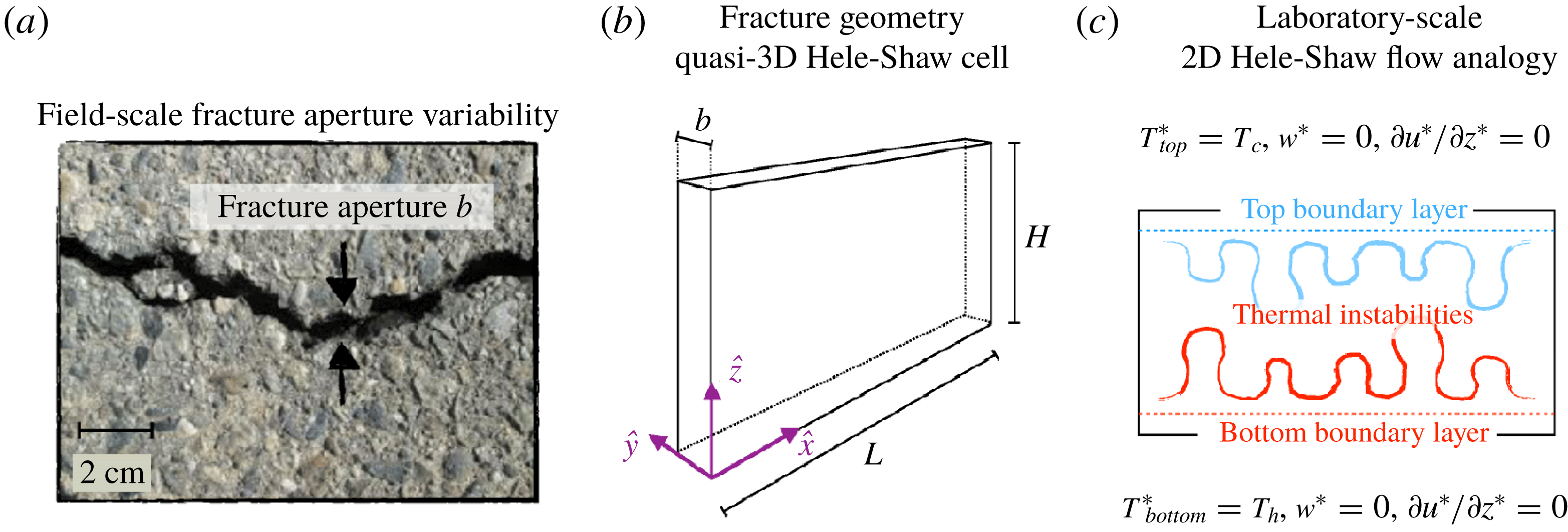
is small but different from zero and fractures can be considered as a quasi-3D geometry. Therefore, the 2D Hele-Shaw flow approximation can be used as an effective model for open fractures that allow the circulation of fluids (see figure 1).
The relation
 $Nu=Nu(Ra)$
for heat transport in the subsurface appears as one of the key physical quantities to be determined. Studies based on numerical simulations of heat transport using the porous media model for the case
 $\unicode[STIX]{x1D6FC}_{L}=\unicode[STIX]{x1D6FC}_{T}=0$
, with Dirichlet conditions for temperature at the bottom and top boundaries, periodic boundary conditions in the horizontal direction and free slip in the vertical direction, demonstrated that for
 $Ra>4\unicode[STIX]{x03C0}^{2}$
the system is unstable and large-scale convective rolls appear, enhancing heat transport (Otero et al.
Reference Otero, Dontcheva, Johnston, Worthing, Kurganov, Petrova and Doering2004; Hewitt et al.
Reference Hewitt, Neufeld and Lister2012). However, for
 $1350<Ra<10\,000$
the quasi-steady convective rolls are unstable and unsteady columnar plumes dominate the dynamics. The case
 $Ra=1350$
marks a transition to an out-of-equilibrium state known as the high-
 $Ra$
regime, where the nonlinear scalings
 $Nu\sim Ra^{0.90}$
and
 $Nu\sim Ra^{0.95}$
have been obtained numerically (Otero et al.
Reference Otero, Dontcheva, Johnston, Worthing, Kurganov, Petrova and Doering2004; Hewitt et al.
Reference Hewitt, Neufeld and Lister2012). For
 $Ra\gtrsim 10^{4}$
, the system exhibits a predominantly vertical exchange flow, where the scaling
 $Nu\sim Ra$
was observed asymptotically (Hewitt et al.
Reference Hewitt, Neufeld and Lister2012).
Geometrical analogy between geological fractures and Hele-Shaw cells. (a) Fracture in a surface at the field scale. Fractures can be open for the circulation of fluids (high permeability), filled by sediments and rocks (reduced permeability) or sealed by mineral deposition (impermeable). In this work, we study open vertical fractures. (b) Fracture geometry used in this work (Murphy Reference Murphy1979). (c) Representation of the problem using a 2D Hele-Shaw flow.

As regards heat transport in Hele-Shaw cells, experimental observations of the scaling
 $Nu\sim Ra^{\unicode[STIX]{x1D6FE}}$
, in conditions where temperature is fixed on the bottom and the cell is open on the top, have been reported by Cherkaoui & Wilcock (Reference Cherkaoui and Wilcock2001) and Cooper et al. (Reference Cooper, Crews, Schumer, Breitmeyer, Voepel and Decker2014) for cases where
 $Ra$
is low (
 $Ra\sim 50$
) to moderate (
 $Ra\sim 1000$
). On the other hand, experimental visualizations of convective cells dominated by plumes in vertical Hele-Shaw cells have been reported recently using fixed-temperature conditions on the bottom and top of the cell (Letelier et al.
Reference Letelier, Herrera, Mujica and Ortega2016). Similar thermal convection has been reported at the field scale (Scheck-Wenderoth et al.
Reference Scheck-Wenderoth, Cacace, Petrovich, Cherubini, Noack, Onno, Sippel and Bjorn2014), where thermal plumes within geological fractures rise from the rock basement, creating convective cells similar to those observed in Hele-Shaw geometries. However, the variability of the fracture aperture induces spatial variations in heat transport (Nigon, Englert & Pascal Reference Nigon, Englert and Pascal2015). The aperture variability can be modelled by the Hele-Shaw geometry through the cell anisotropy ratio
 $\unicode[STIX]{x1D716}$
, as we have indicated previously. Kvernvold & Tyvand (Reference Kvernvold and Tyvand1981) incorporated in the porous media model the dimensionless mechanical dispersion tensor for Hele-Shaw cells given by the coefficients
 $\unicode[STIX]{x1D6FC}_{L}=(2/35)\unicode[STIX]{x1D716}^{2}\,|\boldsymbol{u}|$
and
 $\unicode[STIX]{x1D6FC}_{T}=0$
, observing a slight decrease in heat transport for
 $Ra<400$
and
 $\unicode[STIX]{x1D716}\sim 0.1$
. For
 $\unicode[STIX]{x1D716}\sim 0.01$
, the effects of dispersion are negligible. This observation motivates the present work, because the porous media model studied numerically by Otero et al. (Reference Otero, Dontcheva, Johnston, Worthing, Kurganov, Petrova and Doering2004) and Hewitt et al. (Reference Hewitt, Neufeld and Lister2012), for the case
 $\unicode[STIX]{x1D6FC}_{L}=\unicode[STIX]{x1D6FC}_{T}=0$
, does not predict a decrease in heat transport due to variations of the cell gap, so their results cannot be applicable to Hele-Shaw flows. In the literature, there are many works showing that the Hele-Shaw geometry incorporates the mechanical dispersion in the scalar equation (Oltean et al.
Reference Oltean, Felder, Panfilov and Bues2004; Oltean, Golfier & Bues Reference Oltean, Golfier and Bues2008) and inertial corrections in the Darcy equation (Bizon et al.
Reference Bizon, Werne, Predtechensky, Julien, McCormick, Swift and Swinney1997; Gondret & Rabaud Reference Gondret and Rabaud1997; Ruyer-Quil Reference Ruyer-Quil2001). For thermal convection in Hele-Shaw geometries, the combination of dispersion and inertial terms in a unique system of equations could induce perturbations in the scaling law
 $Nu\sim Ra^{\unicode[STIX]{x1D6FE}(\unicode[STIX]{x1D716})}$
, valid for the high-
 $Ra$
regime, that have not been quantified rigorously.
In this work, we study numerically the fluid dynamics of heat transport using a 2D model valid for vertical Hele-Shaw geometries, derived from first principles, with the aim of quantifying the effects of mechanical dispersion and inertial corrections in heat transport. The main contribution of this article is to show that the Hele-Shaw flow, which incorporates the mechanical dispersion and inertial corrections in the porous media model, gives new scalings for heat transport and total thermal dissipation rate (also called mean scalar dissipation rate in two-fluid mixing problems (Hidalgo et al.
Reference Hidalgo, Fe, Cueto-Felgueroso and Juanes2012)) in the high-
 $Ra$
regime, which are valid for
 $\unicode[STIX]{x1D716}^{2}Ra\ll 1$
.
The article is structured as follows. In § 2 the 2D set of equations for heat transport in vertical Hele-Shaw geometries and boundary conditions are presented. In § 3 we derive mathematical expressions for the Nusselt number and total thermal dissipation rate to study globally heat transport in Hele-Shaw cells. Finally, in § 4 we show the results of the numerical simulations and discuss the potential applications of these results to geothermal convection in vertical fractures.
2 Mathematical model
The representation of natural convection inside vertical geological fractures can be modelled using a 3D rectangular Hele-Shaw geometry heated at the bottom and top with constant temperatures
 $T_{h}$
and
 $T_{c}$
, respectively, with
 $T_{c}<T_{h}$
, and filled with a fluid of constant viscosity
 $\unicode[STIX]{x1D707}$
and density
 $\unicode[STIX]{x1D70C}^{\ast }=\unicode[STIX]{x1D70C}_{c}-\unicode[STIX]{x1D6FC}(T^{\ast }-T_{c})$
, where
 $T^{\ast }$
is the temperature,
 $\unicode[STIX]{x1D6FC}$
is the thermal expansion coefficient and
 $\unicode[STIX]{x1D70C}_{c}$
is the density at the temperature
 $T_{c}$
. The size of the geometry is
 $b\times H\times L$
, where
 $b$
is the cell gap in the
 ${\hat{y}}$
direction,
 $H$
is the height in the
 $\hat{z}$
direction and
 $L$
is the width in the
 $\hat{x}$
direction. For
 $b\ll H$
, the fluid motion is described by the effective 2D model (Hele-Shaw equations)
 $$\begin{eqnarray}\displaystyle & \displaystyle \unicode[STIX]{x1D6FB}^{\ast }\boldsymbol{\cdot }\boldsymbol{u}^{\ast }=0, & \displaystyle\end{eqnarray}$$
 $$\begin{eqnarray}\displaystyle & \displaystyle \unicode[STIX]{x1D70C}_{c}\left(\frac{6}{5}\frac{\unicode[STIX]{x2202}\boldsymbol{u}^{\ast }}{\unicode[STIX]{x2202}t^{\ast }}+\frac{54}{35}(\boldsymbol{u}^{\ast }\boldsymbol{\cdot }\unicode[STIX]{x1D6FB}^{\ast })\boldsymbol{u}^{\ast }\right)=-\unicode[STIX]{x1D6FB}^{\ast }\tilde{p}^{\ast }-\frac{\unicode[STIX]{x1D707}}{K}\boldsymbol{u}^{\ast }+\unicode[STIX]{x1D6FC}(T^{\ast }-T_{c})g\hat{z}+\frac{6}{5}\unicode[STIX]{x1D707}\unicode[STIX]{x1D6FB}^{\ast 2}\boldsymbol{u}^{\ast }-\boldsymbol{L}_{adv}, & \displaystyle \nonumber\\ \displaystyle & & \displaystyle\end{eqnarray}$$
 $$\begin{eqnarray}\displaystyle & \displaystyle \frac{\unicode[STIX]{x2202}T^{\ast }}{\unicode[STIX]{x2202}t^{\ast }}+\boldsymbol{u}^{\ast }\boldsymbol{\cdot }\unicode[STIX]{x1D6FB}^{\ast }T^{\ast }=\unicode[STIX]{x1D705}\unicode[STIX]{x1D6FB}^{\ast 2}T^{\ast }+\frac{2}{35}\frac{K}{\unicode[STIX]{x1D705}}\unicode[STIX]{x1D6FB}^{\ast }\cdot [(\boldsymbol{u}^{\ast }\boldsymbol{\cdot }\unicode[STIX]{x1D6FB}^{\ast }T^{\ast })\boldsymbol{u}^{\ast }], & \displaystyle\end{eqnarray}$$
where the vector
 $\boldsymbol{L}_{adv}$
is the vertical advection term
 $$\begin{eqnarray}\displaystyle \boldsymbol{L}_{adv}=\frac{2}{35}\frac{\unicode[STIX]{x1D6FC}gK}{\unicode[STIX]{x1D705}}(\boldsymbol{u}^{\ast }\boldsymbol{\cdot }\unicode[STIX]{x1D6FB}^{\ast }T^{\ast })\hat{z}. & & \displaystyle\end{eqnarray}$$
For the problem studied in this work, these equations were derived from the 3D incompressible Navier–Stokes model coupled with the advection–diffusion equation for heat transport by using regular perturbation theory, which is shown in appendix A. The left-hand side of (2.2) is the inertial correction derived by Ruyer-Quil (Reference Ruyer-Quil2001) in the context of shear flows in Hele-Shaw cells. Assuming
 $\boldsymbol{L}_{adv}=\mathbf{0}$
, the right-hand side of (2.2) is the Darcy–Brinkman extension for convection problems. Finally, the right-hand side of (2.3) is the hydrodynamic dispersion for this kind of geometry (Oltean et al.
Reference Oltean, Felder, Panfilov and Bues2004). In terms of the Scheidegger dispersion tensor, the dispersion coefficients are
 $\unicode[STIX]{x1D6FC}_{L}=(2/35)(K/\unicode[STIX]{x1D705})|\boldsymbol{u}^{\ast }|$
and
 $\unicode[STIX]{x1D6FC}_{T}=0$
. The boundary conditions assumed for this problem are periodic in
 $x$
-axis,
 $w^{\ast }=0$
,
 $\unicode[STIX]{x2202}u^{\ast }/\unicode[STIX]{x2202}z^{\ast }=0$
and
 $T^{\ast }=T_{h}$
at
 $z^{\ast }=0$
,
 $w^{\ast }=0$
,
 $\unicode[STIX]{x2202}u^{\ast }/\unicode[STIX]{x2202}z^{\ast }=0$
and
 $T^{\ast }=T_{c}$
at
 $z^{\ast }=H$
. These boundary conditions were used by Otero et al. (Reference Otero, Dontcheva, Johnston, Worthing, Kurganov, Petrova and Doering2004) and Hewitt et al. (Reference Hewitt, Neufeld and Lister2012) to model thermal convection in porous media. In (2.1)–(2.3),
 $\boldsymbol{x}^{\ast }=x^{\ast }\hat{x}+z^{\ast }\hat{z}$
is the position,
 $\boldsymbol{u}^{\ast }=u^{\ast }\hat{x}+w^{\ast }\hat{z}$
is the velocity field,
 $\tilde{p}^{\ast }=p^{\ast }+\unicode[STIX]{x1D70C}_{c}gz^{\ast }$
is the modified pressure,
 $g$
is the gravitational acceleration and
 $\unicode[STIX]{x1D705}$
is the thermal diffusivity. To make the model dimensionless, we use the scalings for position
 $\boldsymbol{x}=\boldsymbol{x}^{\ast }/H$
, velocity
 $\boldsymbol{u}=\boldsymbol{u}^{\ast }/u_{c}$
, pressure
 $p=\tilde{p}^{\ast }/p_{s}$
, time
 $t=u_{c}t^{\ast }/H$
and temperature
 $T=(T^{\ast }-T_{c})/(T_{h}-T_{c})$
, with
 $K=b^{2}/12$
the cell permeability,
 $u_{c}=\unicode[STIX]{x1D6FC}(T_{h}-T_{c})gK/\unicode[STIX]{x1D707}$
the characteristic velocity and
 $p_{s}=\unicode[STIX]{x1D707}u_{c}H/K$
the characteristic pressure. The dimensionless parameters of the model are the Prandtl number
 $Pr=\unicode[STIX]{x1D708}/\unicode[STIX]{x1D705}$
, the Rayleigh number
 $Ra=u_{c}H/\unicode[STIX]{x1D705}$
and the anisotropy ratio
 $\unicode[STIX]{x1D716}=\sqrt{K}/H$
, with
 $\unicode[STIX]{x1D708}=\unicode[STIX]{x1D707}/\unicode[STIX]{x1D70C}_{c}$
the kinematic viscosity. Therefore, the dimensionless set of equations studied in this work are
 $$\begin{eqnarray}\displaystyle & \displaystyle \unicode[STIX]{x1D735}\boldsymbol{\cdot }\boldsymbol{u}=0, & \displaystyle\end{eqnarray}$$
 $$\begin{eqnarray}\displaystyle & \displaystyle \unicode[STIX]{x1D716}^{2}\frac{Ra}{Pr}\left(\frac{6}{5}\frac{\unicode[STIX]{x2202}\boldsymbol{u}}{\unicode[STIX]{x2202}t}+\frac{54}{35}(\boldsymbol{u}\boldsymbol{\cdot }\unicode[STIX]{x1D735})\boldsymbol{u}\right)=-\unicode[STIX]{x1D735}p-\boldsymbol{u}+T\hat{z}+\frac{6}{5}\unicode[STIX]{x1D716}^{2}\unicode[STIX]{x1D6FB}^{2}\boldsymbol{u}-\frac{2}{35}\unicode[STIX]{x1D716}^{2}Ra(\boldsymbol{u}\boldsymbol{\cdot }\unicode[STIX]{x1D735}T)\hat{z},\qquad & \displaystyle\end{eqnarray}$$
 $$\begin{eqnarray}\displaystyle & \displaystyle \frac{\unicode[STIX]{x2202}T}{\unicode[STIX]{x2202}t}+\boldsymbol{u}\boldsymbol{\cdot }\unicode[STIX]{x1D735}T=\frac{1}{Ra}\unicode[STIX]{x1D6FB}^{2}T+\frac{2}{35}\unicode[STIX]{x1D716}^{2}Ra\unicode[STIX]{x1D735}\boldsymbol{\cdot }[(\boldsymbol{u}\boldsymbol{\cdot }\unicode[STIX]{x1D735}T)\boldsymbol{u}], & \displaystyle\end{eqnarray}$$
valid for
 $\unicode[STIX]{x1D716}$
small,
 $Pr\geqslant 1$
and
 $\unicode[STIX]{x1D716}^{2}Ra\ll 1$
. The boundary conditions are periodic in
 $x$
-axis, while in
 $z$
-axis we assume free-slip boundary conditions,
 $T=1$
at
 $z=0$
and
 $T=0$
at
 $z=1$
.
3 Heat transport and thermal dissipation rate
Using 2D Cartesian tensors, (2.7) can be written as
 $$\begin{eqnarray}\displaystyle \frac{\unicode[STIX]{x2202}T}{\unicode[STIX]{x2202}t}+\unicode[STIX]{x2202}_{j}\unicode[STIX]{x1D6F1}_{j}=\unicode[STIX]{x2202}_{i}({\mathcal{D}}_{ij}\unicode[STIX]{x2202}_{j}T);\quad {\mathcal{D}}_{ij}=\frac{1}{Ra}\unicode[STIX]{x1D6FF}_{ij}+\frac{2}{35}\unicode[STIX]{x1D716}^{2}Ra(u_{i}u_{j}), & & \displaystyle\end{eqnarray}$$
where
 $\unicode[STIX]{x1D6F1}_{j}=u_{j}T$
is the convective heat flux in the
 $j$
-direction,
 $\unicode[STIX]{x2202}_{j}\unicode[STIX]{x1D6F1}_{j}$
is the convective heat flux density (scalar) and
 ${\mathcal{D}}_{ij}$
is the hydrodynamic dispersion tensor, with
 $\unicode[STIX]{x1D6FF}_{ij}$
the Kronecker delta. Now, consider the term
 $\unicode[STIX]{x1D6F7}_{i}=u_{i}u_{j}\unicode[STIX]{x2202}_{j}T$
. Using the equation
 $\unicode[STIX]{x2202}_{i}u_{i}=0$
, we obtain
 $\unicode[STIX]{x1D6F7}_{i}=u_{i}\unicode[STIX]{x2202}_{j}(u_{j}T)=u_{i}\unicode[STIX]{x2202}_{j}\unicode[STIX]{x1D6F1}_{j}$
, so we can see that
 $\unicode[STIX]{x1D6F7}_{i}$
is also a flux in the
 $i$
-direction. In particular,
 $\unicode[STIX]{x1D6F7}_{z}=w\unicode[STIX]{x2202}_{j}(u_{j}T)=w\unicode[STIX]{x1D735}\boldsymbol{\cdot }(\boldsymbol{u}T)$
can be interpreted as the vertical flux of the convective heat density. The Hele-Shaw cell is a quasi-3D geometry where heat flux can also be transported in
 $y$
-axis, i.e. along the cell gap. Assuming
 $\unicode[STIX]{x1D716}\ll 1$
to reduce the 3D Navier–Stokes equation coupled with the scalar transport to the 2D model shown in (2.5)–(2.7), the perturbative effects of the cell gap in the scalar transport equation (3.1) are captured by the flux density
 $\unicode[STIX]{x2202}_{i}\unicode[STIX]{x1D6F7}_{i}$
, i.e. the mechanical dispersion, which causes additional mixing. In porous media, it is well known that mechanical dispersion appears as a response of the detours due to tortuosity and variable routes of the flow in the porous matrix. In our case, mechanical dispersion appears due to the existence of a third confined spatial dimension.
Equation (3.1) can be written as
 $$\begin{eqnarray}\displaystyle \frac{\unicode[STIX]{x2202}T}{\unicode[STIX]{x2202}t}+\unicode[STIX]{x2202}_{i}\left(\unicode[STIX]{x1D6F1}_{i}-\frac{2}{35}\unicode[STIX]{x1D716}^{2}Ra\unicode[STIX]{x1D6F7}_{i}\right)=\frac{1}{Ra}\unicode[STIX]{x1D6FB}^{2}T, & & \displaystyle\end{eqnarray}$$
where we define the net heat flux in the
 $i$
-direction
 $\unicode[STIX]{x1D6F9}_{i}$
as
 $$\begin{eqnarray}\displaystyle \unicode[STIX]{x1D6F9}_{i}=\unicode[STIX]{x1D6F1}_{i}-{\textstyle \frac{2}{35}}\unicode[STIX]{x1D716}^{2}Ra\unicode[STIX]{x1D6F7}_{i}. & & \displaystyle\end{eqnarray}$$
This equation represents the competition of two processes, heat transport and mixing. In particular,
 $\unicode[STIX]{x1D6F1}_{z}$
represents the vertical heat flux, which can be interpreted as the advection of a fluid parcel with constant temperature
 $T$
, but
 $\unicode[STIX]{x1D6F7}_{z}$
can be interpreted as the vertical advection of a fluid parcel that continuously exchanges heat with the surrounding fluid, so the fluid parcel is mixed with other parcels, reaching intermediate temperatures. The net effect is the decrease of global heat transport, due to the minus sign in
 $\unicode[STIX]{x1D6F9}_{z}$
.
3.1 Global heat transport: the Nusselt number
Global heat transport can be computed by averaging (3.2) over the entire domain. Hence, the average in the horizontal direction and the domain average of a function
 $f=f(\boldsymbol{x})$
are defined as
 $\langle f\rangle _{h}(z)=1/L^{\prime }\int _{0}^{L^{\prime }}f(\boldsymbol{x})\,\text{d}x$
and
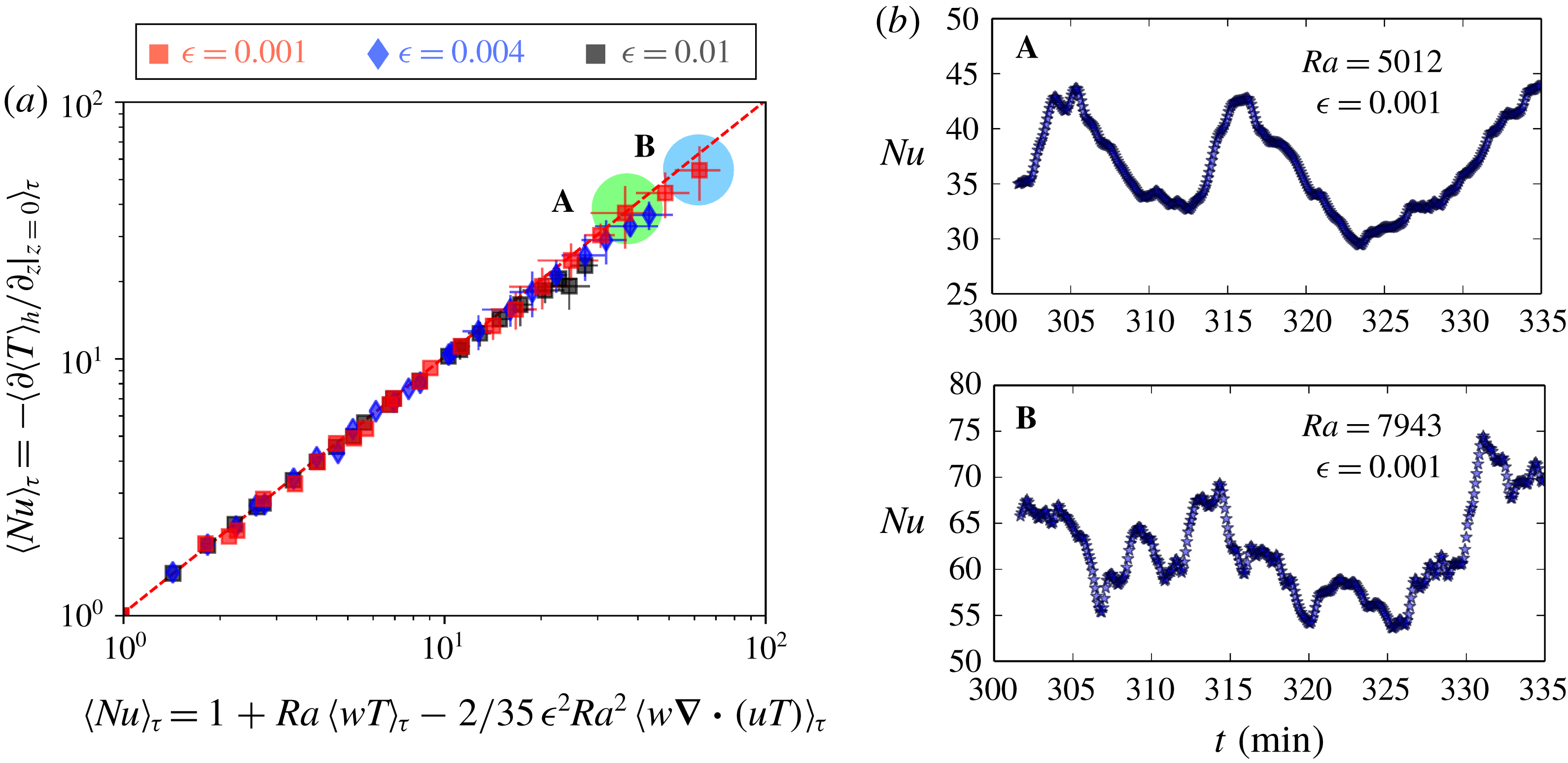
 $\langle f\rangle =\int _{0}^{1}\langle f\rangle _{h}(z)\,\text{d}z$
, respectively, where
 $L^{\prime }=L/H$
is the aspect ratio of the cell. Then, heat transport can be studied by means of the Nusselt number defined as
 $$\begin{eqnarray}\displaystyle \left.Nu=-\frac{\unicode[STIX]{x2202}\langle T\rangle _{h}}{\unicode[STIX]{x2202}z}\right|_{z=0}. & & \displaystyle\end{eqnarray}$$
Assuming periodic boundary conditions for all variables in the horizontal direction, the horizontal average of (3.2) is
 $$\begin{eqnarray}\displaystyle \frac{\unicode[STIX]{x2202}\langle T\rangle _{h}}{\unicode[STIX]{x2202}t}+\unicode[STIX]{x2202}_{z}\langle \unicode[STIX]{x1D6F1}_{z}\rangle _{h}-\frac{2}{35}\unicode[STIX]{x1D716}^{2}Ra\unicode[STIX]{x2202}_{z}\langle \unicode[STIX]{x1D6F7}_{z}\rangle _{h}=\frac{1}{Ra}\unicode[STIX]{x2202}_{z}^{2}\langle T\rangle _{h}. & & \displaystyle\end{eqnarray}$$
In the steady-state regime, and assuming
 $w=0$
in
 $z=0$
and
 $z=1$
, we integrate (3.5) in the vertical direction. Next, evaluating the last equation for
 $z=0$
and using (3.4), we obtain an expression for the Nusselt number given by the formula
 $$\begin{eqnarray}\displaystyle Nu=1+Ra\langle wT\rangle -{\textstyle \frac{2}{35}}\unicode[STIX]{x1D716}^{2}Ra^{2}\langle w\unicode[STIX]{x1D735}\boldsymbol{\cdot }(\boldsymbol{u}T)\rangle , & & \displaystyle\end{eqnarray}$$
which includes the contribution of the perturbative corrections through the second-order correction
 $\unicode[STIX]{x1D716}^{2}Ra^{2}\langle \unicode[STIX]{x1D6F7}_{z}\rangle$
. The Nusselt number given in (3.6) is time-dependent, so the time-averaged Nusselt number
 $\langle Nu\rangle _{\unicode[STIX]{x1D70F}}$
, defined in appendix B, will be the dimensionless number that quantifies global heat transport. This computation is done at times
 $t\gg 1$
to ensure that a statistical stationary behaviour is reached by the system. When
 $\unicode[STIX]{x1D716}=0$
, we obtain the usual Nusselt definition given in the literature
 $Nu=1+Ra\langle wT\rangle$
(Nield & Bejan Reference Nield and Bejan2006).
3.2 Total thermal dissipation rate
The next step is to derive an equation for thermal dissipation. Multiplying both sides of the dimensionless form of (2.7) by
 $T$
and after an algebraic manipulation, we obtain the formulas
 $$\begin{eqnarray}\displaystyle & \displaystyle \frac{1}{2}\frac{\unicode[STIX]{x2202}(T^{2})}{\unicode[STIX]{x2202}t}+\unicode[STIX]{x1D735}\boldsymbol{\cdot }{\mathcal{T}}_{e}=-\unicode[STIX]{x1D717}, & \displaystyle\end{eqnarray}$$
 $$\begin{eqnarray}\displaystyle & \displaystyle {\mathcal{T}}_{e}=\frac{1}{2}\boldsymbol{u}T^{2}-\frac{1}{Ra}T\unicode[STIX]{x1D735}T-\frac{2}{35}\unicode[STIX]{x1D716}^{2}Ra[(\unicode[STIX]{x1D735}\boldsymbol{\cdot }(\boldsymbol{u}T))\boldsymbol{u}T], & \displaystyle\end{eqnarray}$$
 $$\begin{eqnarray}\displaystyle & \displaystyle \unicode[STIX]{x1D717}=\frac{1}{Ra}\Vert \unicode[STIX]{x1D735}T\Vert ^{2}+\frac{2}{35}\unicode[STIX]{x1D716}^{2}Ra(\unicode[STIX]{x1D735}\boldsymbol{\cdot }(\boldsymbol{u}T))^{2}, & \displaystyle\end{eqnarray}$$
where
 ${\mathcal{T}}_{e}$
is the thermal transfer function associated with heat transport and
 $\unicode[STIX]{x1D717}$
is the local thermal dissipation rate due to heat convection. The thermal dissipation rate is the analogue of the well-known scalar dissipation rate in fluid mixing (Jha, Cueto-Felgueroso & Juanes Reference Jha, Cueto-Felgueroso and Juanes2011; Hidalgo et al.
Reference Hidalgo, Fe, Cueto-Felgueroso and Juanes2012; Jha, Cueto-Felgueroso & Juanes Reference Jha, Cueto-Felgueroso and Juanes2013; Pramanik & Mishra Reference Pramanik and Mishra2015), and it represents a measure of the irreversibility of heat transfer processes. Using the free-slip boundary conditions of the problem, applying the domain average defined in § 3.1 and assuming a permanent regime for time variation, equation (3.7) is written as
 $$\begin{eqnarray}\displaystyle \frac{1}{L^{\prime }}\int _{0}^{L^{\prime }}\int _{0}^{1}\left[\frac{\unicode[STIX]{x2202}}{\unicode[STIX]{x2202}x}\left(T\frac{\unicode[STIX]{x2202}^{}T_{}}{\unicode[STIX]{x2202}x^{}}\right)+\frac{\unicode[STIX]{x2202}}{\unicode[STIX]{x2202}z}\left(T\frac{\unicode[STIX]{x2202}^{}T_{}}{\unicode[STIX]{x2202}z^{}}\right)\right]\,\text{d}x\,\text{d}z=\frac{Ra}{L^{\prime }}\int _{0}^{L^{\prime }}\int _{0}^{1}\unicode[STIX]{x1D717}\,\text{d}x\,\text{d}z. & & \displaystyle\end{eqnarray}$$
Applying the boundary conditions for the temperature, the above equation is reduced to the formula
 $$\begin{eqnarray}\displaystyle \left.-\frac{1}{L^{\prime }}\int _{0}^{L^{\prime }}\frac{\unicode[STIX]{x2202}^{}T_{}}{\unicode[STIX]{x2202}z^{}}\right|_{z=0}\,\text{d}x=\frac{Ra}{L^{\prime }}\int _{0}^{L^{\prime }}\int _{0}^{1}\unicode[STIX]{x1D717}\,\text{d}x\,\text{d}z\quad \Longrightarrow \quad \left.-\frac{\unicode[STIX]{x2202}\langle T\rangle _{h}}{\unicode[STIX]{x2202}z}\right|_{z=0}=Ra\langle \unicode[STIX]{x1D717}\rangle , & & \displaystyle\end{eqnarray}$$
where
 $\langle \unicode[STIX]{x1D717}\rangle$
is the total thermal dissipation rate
 $$\begin{eqnarray}\displaystyle \langle \unicode[STIX]{x1D717}\rangle =\frac{1}{Ra}\langle \Vert \unicode[STIX]{x1D735}T\Vert ^{2}\rangle +\frac{2}{35}\unicode[STIX]{x1D716}^{2}Ra\langle (\unicode[STIX]{x1D735}\boldsymbol{\cdot }(\boldsymbol{u}T))^{2}\rangle . & & \displaystyle\end{eqnarray}$$
Finally, using (3.4) and applying the time-average formula defined in appendix B, we obtain
 $$\begin{eqnarray}\displaystyle \langle Nu\rangle _{\unicode[STIX]{x1D70F}}=Ra\langle \unicode[STIX]{x1D717}\rangle _{\unicode[STIX]{x1D70F}}. & & \displaystyle\end{eqnarray}$$
Equation (3.13) is important, because it establishes a theoretical scaling relation between heat transport and total thermal dissipation rate, being a generalization of the scalings reported by Otero et al. (Reference Otero, Dontcheva, Johnston, Worthing, Kurganov, Petrova and Doering2004) and Hewitt et al. (Reference Hewitt, Neufeld and Lister2012), and it is independent of the effects of the perturbative corrections, which appear explicitly in
 $Nu$
and
 $\langle \unicode[STIX]{x1D717}\rangle$
. From the results reported by Hewitt et al. (Reference Hewitt, Neufeld and Lister2012) using the Darcy model, the asymptotic scaling for heat transport is
 $\langle Nu\rangle _{\unicode[STIX]{x1D70F}}\sim Ra$
, which is valid for the ultimate
 $Ra$
regime in porous media. Using (3.13), we conclude that
 $\langle \unicode[STIX]{x1D717}\rangle _{\unicode[STIX]{x1D70F}}$
must be independent of
 $Ra$
, which is a result reported by Jenny et al. (Reference Jenny, Lee, Meyer and Tchelepi2014) in the context of mass transfer.
4 Numerical simulations
Since we are interested in analysing the effects of the perturbative corrections in the development of convection, i.e. mechanical dispersion and inertial corrections, we compare heat transport properties of the proposed Hele-Shaw model, equations (2.5)–(2.7), with published results of Otero et al. (Reference Otero, Dontcheva, Johnston, Worthing, Kurganov, Petrova and Doering2004) and Hewitt et al. (Reference Hewitt, Neufeld and Lister2012). We performed direct numerical simulations using the spectrally based software flow_solve (Winters & de la Fuente Reference Winters and de la Fuente2012), which has been applied to geophysical fluid dynamics problems such as wave instabilities in the atmosphere and ocean, large-scale tidal phenomena and transition to turbulence in two and three dimensions. The software was implemented using FORTRAN and MPI libraries for parallel computing. The discretization of equations is based on trigonometric and Fourier expansions, so the software is good for problems with free-slip boundary conditions. We have used this software due to its excellent capabilities in parallel computing and high numerical resolution. The main dimensionless parameters that are fixed in numerical simulations are the anisotropy ratio
 $\unicode[STIX]{x1D716}$
, the Prandtl number
 $Pr$
and the aspect ratio
 $L^{\prime }=L/H$
, while
 $Ra$
varies from from
 $40$
to
 $10^{4}$
. For all simulations,
 $Pr=7$
.
We define the conductive base state as
 $u_{s}=0$
,
 $w_{s}=0$
and
 $T_{s}(z)=1-z$
. Then, we perturbe all dynamical variables as
 $u(\boldsymbol{x},t)=0+u^{\prime }(\boldsymbol{x},t)$
,
 $w(\boldsymbol{x},t)=0+w^{\prime }(\boldsymbol{x},t)$
,
 $p(\boldsymbol{x},t)=p_{s}(z)+p^{\prime }(\boldsymbol{x},t)$
and
 $T(\boldsymbol{x},t)=T_{s}(z)+\unicode[STIX]{x1D703}(\boldsymbol{x},t)$
, where density and pressure base states satisfy the hydrostatic equation
 $\text{d}p_{s}/\text{d}z=-T_{s}(z)$
. The boundary conditions are periodic in
 $x$
-axis, while for
 $z$
-axis we have
 $w=0$
,
 $\unicode[STIX]{x2202}u/\unicode[STIX]{x2202}z=0$
and
 $\unicode[STIX]{x1D703}=0$
in
 $z=0$
and
 $z=1$
. Then, we expand
 $u^{\prime }\sim \exp (ik_{n}x)\cos (n\unicode[STIX]{x03C0}z)$
,
 $w^{\prime }\sim \exp (ik_{n}x)\sin (n\unicode[STIX]{x03C0}z)$
and
 $\unicode[STIX]{x1D703}\sim \exp (ik_{n}x)\sin (n\unicode[STIX]{x03C0}z)$
, where
 $n$
is a natural number and
 $k_{n}$
is the wavenumber.
The spatial resolution of the simulations is computed as
 $\unicode[STIX]{x0394}x=L/n_{x}$
and
 $\unicode[STIX]{x0394}z=H/(n_{z}+1)$
, where
 $n_{x}$
and
 $n_{z}$
are the grid points which depend on
 $Ra$
. For example, in domains with aspect ratio
 $L^{\prime }=L/H=2$
, we have
 $n_{x}=2n_{z}=64$
for small
 $Ra$
and
 $n_{x}=2n_{z}=512$
to
 $1024$
for high
 $Ra$
. In each case, the number of grid points was choosen to ensure aproximately six points within the boundary layer. To generate thermal instabilities, we trigger a small perturbation through the following initial conditions for velocity components and temperature:
 $$\begin{eqnarray}\displaystyle & \displaystyle \boldsymbol{u}^{\prime }(\boldsymbol{x},t=0)=\mathbf{0}, & \displaystyle\end{eqnarray}$$
 $$\begin{eqnarray}\displaystyle & \displaystyle \unicode[STIX]{x1D703}(\boldsymbol{x},t=0)=A\;\text{rand}(x)[\exp (-z^{2}/\unicode[STIX]{x1D70E}_{z}^{2})+\exp (-(z-1)^{2}/\unicode[STIX]{x1D70E}_{z}^{2})], & \displaystyle\end{eqnarray}$$
where
 $\text{rand}(x)\in [-1,1]$
is the uniform distribution and
 $A$
is a small parameter. Finally, to compute the gradient and divergence operators for heat transport estimation, we use fourth-order compact finite differences with high spectral resolution (Lele Reference Lele1992). The time step is defined satisfying the Courant–Friedrichs–Lewy (CFL) condition. In general, the CFL value is
 $0.06$
for moderate
 $Ra$
and
 $0.01$
for high
 $Ra$
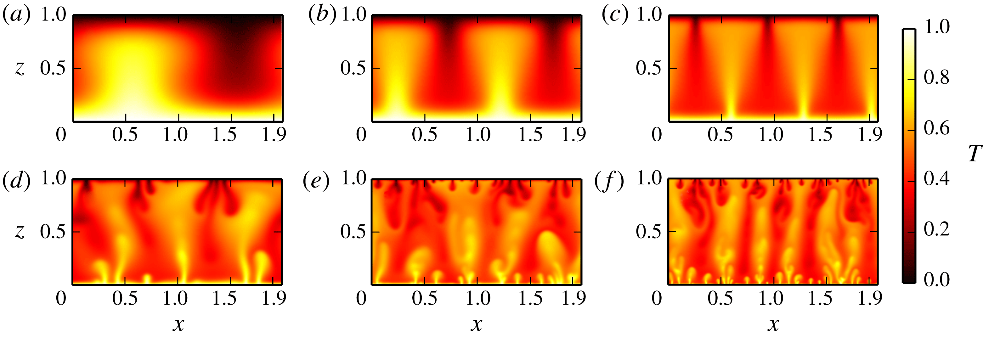
. Examples of our results are presented in figure 2. In this figure, some features of the temperature distribution are displayed, when diffusion and mechanical dispersion terms in (2.7) are comparable.
Numerical simulation results with
 $L^{\prime }=L/H=2$
, for
 $Pr=7$
. (a) Unicellular steady convection for
 $\unicode[STIX]{x1D716}=4.18\times 10^{-2}$
and
 $Ra=100$
, (b) bicellular steady convection for
 $\unicode[STIX]{x1D716}=1.32\times 10^{-2}$
and
 $Ra=316$
and (c) tricellular steady convection for
 $\unicode[STIX]{x1D716}=4.18\times 10^{-3}$
and
 $Ra=1000$
. Unsteady dynamics: (d) for
 $\unicode[STIX]{x1D716}=1.67\times 10^{-3}$
and
 $Ra=2512$
, (e) for
 $\unicode[STIX]{x1D716}=8.35\times 10^{-4}$
and
 $Ra=5012$
and (f) for
 $\unicode[STIX]{x1D716}=5.27\times 10^{-4}$
and
 $Ra=7943$
.

Parameter
 $\langle Nu\rangle _{\unicode[STIX]{x1D70F}}$
as a function of
 $Ra$
, for
 $Pr=7$
and
 $L^{\prime }=2$
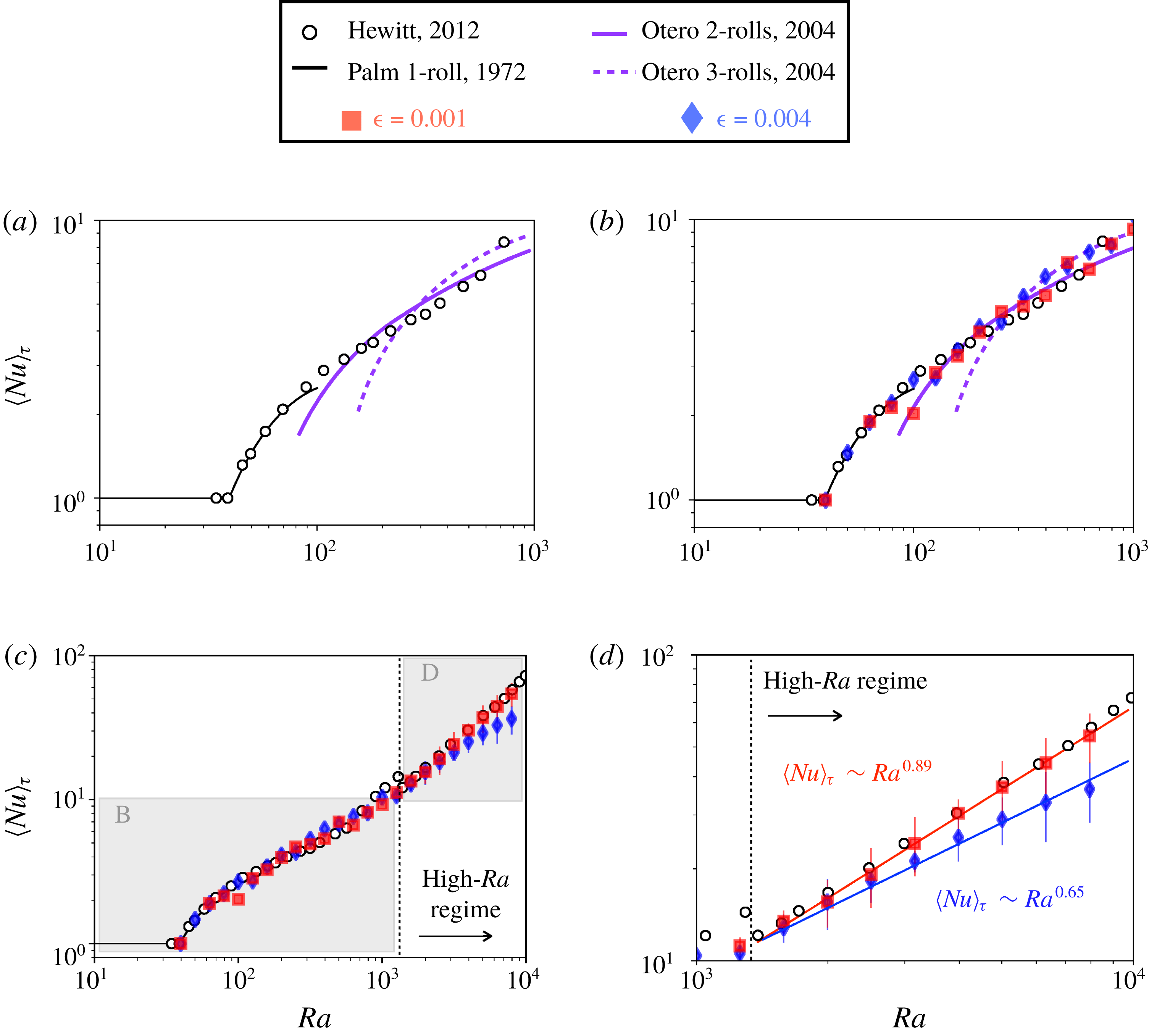
. (a) Results obtained by Hewitt et al. (Reference Hewitt, Neufeld and Lister2012) using the porous media model, and trajectories for 1-roll, 2-rolls and 3-rolls obtained by Palm, Weber & Kvernvold (Reference Palm, Weber and Kvernvold1972) and Otero et al. (Reference Otero, Dontcheva, Johnston, Worthing, Kurganov, Petrova and Doering2004). (b) Our results for two sets of simulations,
 $\unicode[STIX]{x1D716}=0.001$
and
 $\unicode[STIX]{x1D716}=0.004$
, which are consistent with previously published results shown in (a). However, for
 $Ra>1350$
, there is a deviation from the Darcy high-
 $Ra$
regime obtained by Hewitt et al. (Reference Hewitt, Neufeld and Lister2012), which depends on
 $\unicode[STIX]{x1D716}$
(c,d). In the high-
 $Ra$
regime (d), scaling is represented by
 $\langle Nu\rangle _{\unicode[STIX]{x1D70F}}\sim Ra^{\unicode[STIX]{x1D6FE}}$
. For
 $\unicode[STIX]{x1D716}=0.004$
the best fit is
 $\unicode[STIX]{x1D6FE}\sim 0.65$
, while for
 $\unicode[STIX]{x1D716}=0.001$
we have
 $\unicode[STIX]{x1D6FE}\sim 0.89$
. Error bars were amplified by a factor of two.

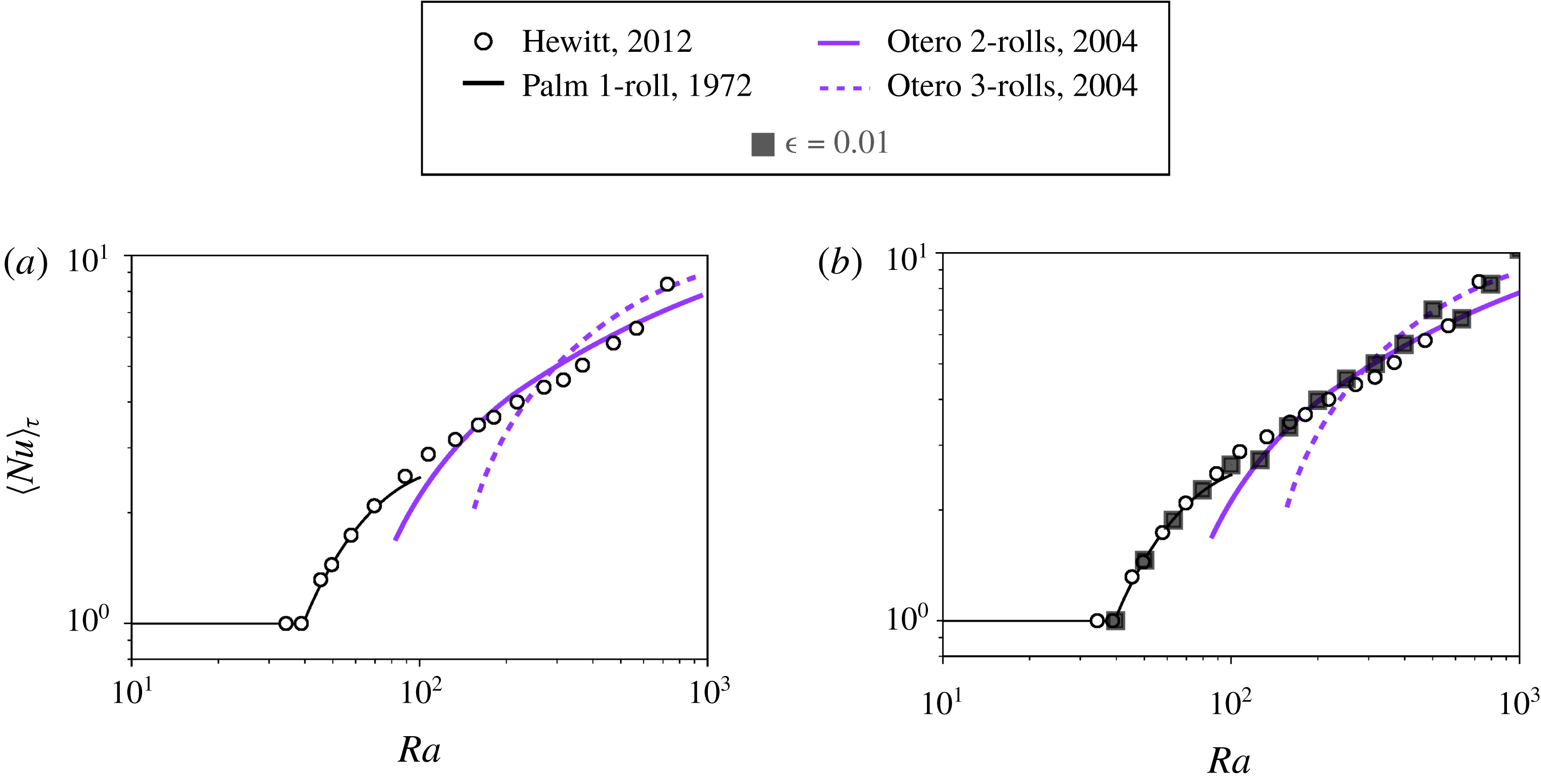
(a) Parameter
 $\langle Nu\rangle _{\unicode[STIX]{x1D70F}}$
as a function of
 $Ra$
, for
 $Pr=7$
and
 $L^{\prime }=2$
. (b) Our results for
 $\unicode[STIX]{x1D716}=0.01$
, which are in agreement with data reported by Palm et al. (Reference Palm, Weber and Kvernvold1972), Otero et al. (Reference Otero, Dontcheva, Johnston, Worthing, Kurganov, Petrova and Doering2004) and Hewitt et al. (Reference Hewitt, Neufeld and Lister2012) (given in (a)).

Physical interpretation of the validity of the 2D model. The shape of thermal plumes
 $\unicode[STIX]{x1D706}$
depends on
 $Ra$
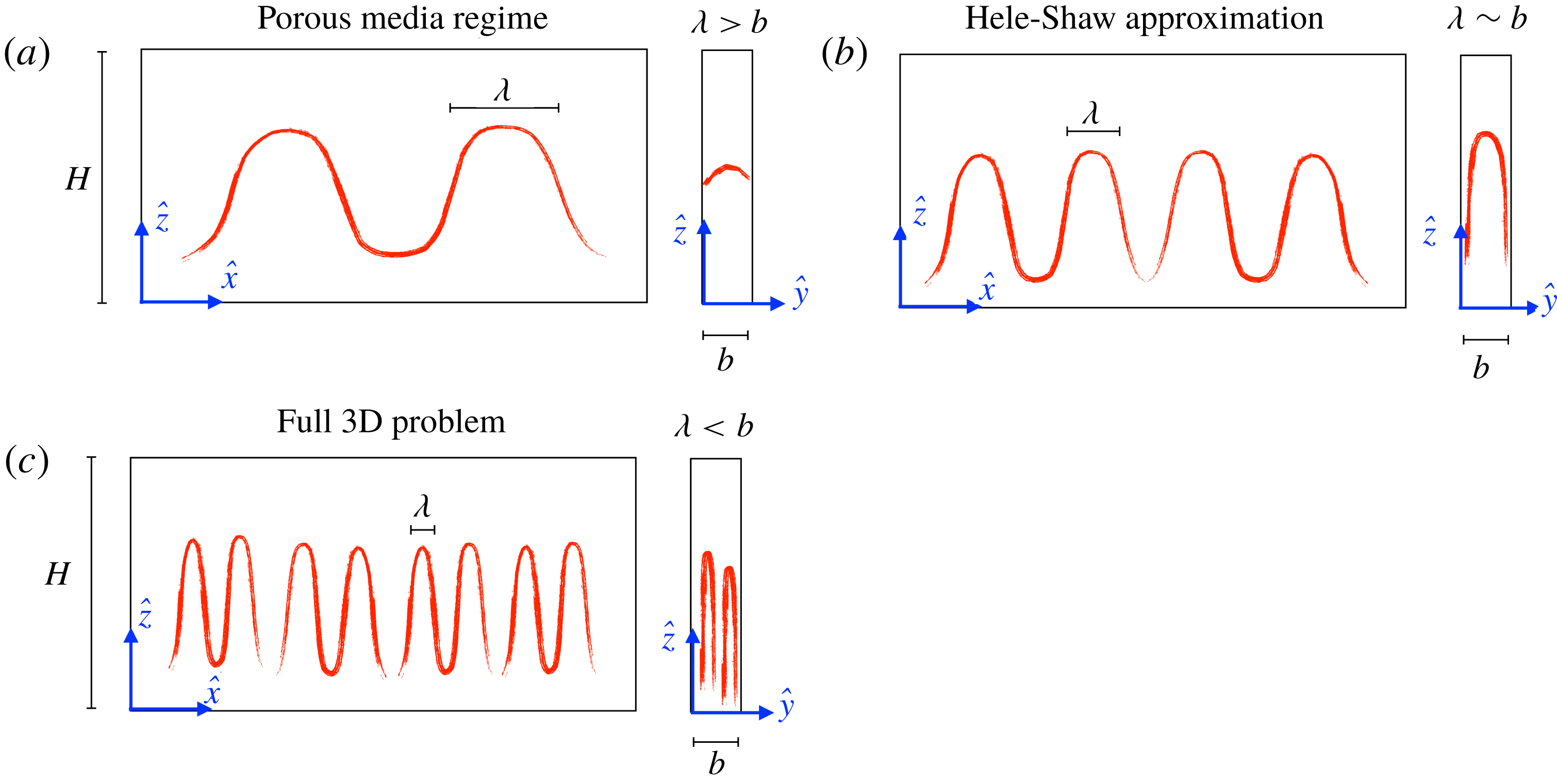
, as shown in figure 2. For the problem context, the porous media regime is valid when the shape of thermal plumes is greater than the cell gap (a). On the other hand, the full 3D problem appears when the shape of thermal plumes is less than the cell gap (c). The intermediate case represents the Hele-Shaw approximation (b).

Figures 3 and 4 show the time-averaged
 $\langle Nu\rangle _{\unicode[STIX]{x1D70F}}$
–
 $Ra$
relation for fixed
 $\unicode[STIX]{x1D716}$
,
 $Pr$
and
 $L^{\prime }$
, obtained by our numerical simulations using (3.6), which are compared with previously published results. We have performed three simulation sets, for
 $\unicode[STIX]{x1D716}=0.01$
,
 $\unicode[STIX]{x1D716}=0.004$
and
 $\unicode[STIX]{x1D716}=0.001$
, which were chosen based on experimental studies (Elder Reference Elder1967; Cherkaoui & Wilcock Reference Cherkaoui and Wilcock2001; Cooper et al.
Reference Cooper, Crews, Schumer, Breitmeyer, Voepel and Decker2014; Letelier et al.
Reference Letelier, Herrera, Mujica and Ortega2016). For all cases mentioned above, we initialize the velocity and temperature fields using (4.1) and (4.2). The convection onset is near to the standard prediction
 $Ra^{(c)}=4\unicode[STIX]{x03C0}^{2}$
, which is expected because of the very small influence of mechanical dispersion and inertial corrections in such a regime. Furthermore, for
 $4\unicode[STIX]{x03C0}^{2}<Ra<1350$
, our results agree with steady convective rolls states previously reported (Nield & Bejan Reference Nield and Bejan2006; Otero et al.
Reference Otero, Dontcheva, Johnston, Worthing, Kurganov, Petrova and Doering2004; Hewitt et al.
Reference Hewitt, Neufeld and Lister2012). However, at higher
 $Ra$
there is a clear separation of the
 $\langle Nu\rangle _{\unicode[STIX]{x1D70F}}$
–
 $Ra$
scaling, which now depends on
 $\unicode[STIX]{x1D716}$
. The scaling is represented by
 $\langle Nu\rangle _{\unicode[STIX]{x1D70F}}\sim Ra^{\unicode[STIX]{x1D6FE}}$
. For
 $\unicode[STIX]{x1D716}=0.004$
the best fit is
 $\unicode[STIX]{x1D6FE}=0.6522\pm 0.0005$
, while for
 $\unicode[STIX]{x1D716}=0.001$
we have
 $\unicode[STIX]{x1D6FE}=0.8894\pm 0.0003$
, which is close to the prediction given by Otero et al. (Reference Otero, Dontcheva, Johnston, Worthing, Kurganov, Petrova and Doering2004). Evidently, the perturbative corrections induced by the cell aperture reduce heat transport because the cell gap effects, captured by the perturbative corrections, aid in homogenization of the temperature, as was discussed in § 3.
The Hele-Shaw model is valid for
 $\unicode[STIX]{x1D716}^{2}Ra\ll 1$
. For
 $\unicode[STIX]{x1D716}=0.001$
, the model works for
 $Ra\ll 10^{6}$
, which is satisfied by our simulations. For
 $\unicode[STIX]{x1D716}=0.004$
,
 $Ra\ll 10^{5}$
, which is also satisfied, but for
 $\unicode[STIX]{x1D716}=0.01$
,
 $Ra\ll 10^{4}$
, the upper value of the Rayleigh number for our simulations. For this case, the results for
 $Ra<1000$
are valid (see figure 4). Figure 5 shows the physical interpretation of the results depicted in figures 3 and 4. For
 $Ra\geqslant 4\unicode[STIX]{x03C0}^{2}$
, the shape of a thermal plume, which is a function of
 $Ra$
, is very large in comparison to the cell gap, so perturbative effects are negligible. This case is similar to considering
 $\unicode[STIX]{x1D716}=0$
in the 2D governing equations. If
 $Ra$
increases but
 $\unicode[STIX]{x1D716}^{2}Ra\ll 1$
, there will be a moment where the shape of a thermal plume can be compared with the cell gap, i.e.
 $\unicode[STIX]{x1D706}\sim b$
. At this moment, mixture processes along the cell gap cannot be neglected and the problem can be treated perturbatively. Thus, the mechanical dispersion and inertial corrections to the porous media model begin to be important. For very large
 $Ra\sim O(1/\unicode[STIX]{x1D716}^{2})$
, the problem is fully 3D. Therefore, for the high-
 $Ra$
regime, there are perturbative corrections in the scaling
 $\langle Nu\rangle _{\unicode[STIX]{x1D70F}}=Ra^{\unicode[STIX]{x1D6FE}(\unicode[STIX]{x1D716})}$
for
 $\unicode[STIX]{x1D716}^{2}Ra\ll 1$
. In the high-
 $Ra$
regime, for
 $\unicode[STIX]{x1D716}\gg 10^{-2}$
, our model cannot be applied.
Parameter
 $\langle \unicode[STIX]{x1D717}\rangle _{\unicode[STIX]{x1D70F}}$
as a function of
 $Ra$
in the high-
 $Ra$
number regime, for
 $Pr=7$
and
 $L^{\prime }=2$
. While the standard model predicts
 $\langle \unicode[STIX]{x1D717}\rangle _{\unicode[STIX]{x1D70F}}$
independent of
 $Ra$
, our model shows that
 $\langle \unicode[STIX]{x1D717}\rangle _{\unicode[STIX]{x1D70F}}$
exhibits a nonlinear scaling with
 $Ra$
that depends on
 $\unicode[STIX]{x1D716}$
values. Plots (a,c,e) show
 $\unicode[STIX]{x1D717}(\boldsymbol{x})$
for
 $\unicode[STIX]{x1D716}=0.01$
and
 $Ra=3162$
,
 $Ra=5012$
and
 $Ra=7943$
, respectively, while plots (b,d,f) show
 $\unicode[STIX]{x1D717}(\boldsymbol{x})$
for
 $\unicode[STIX]{x1D716}=0.001$
and
 $Ra=3162$
,
 $Ra=5012$
and
 $Ra=7943$
, respectively.

Figure 6 shows the
 $\langle \unicode[STIX]{x1D717}\rangle _{\unicode[STIX]{x1D70F}}$
–
 $Ra$
scaling at high
 $Ra$
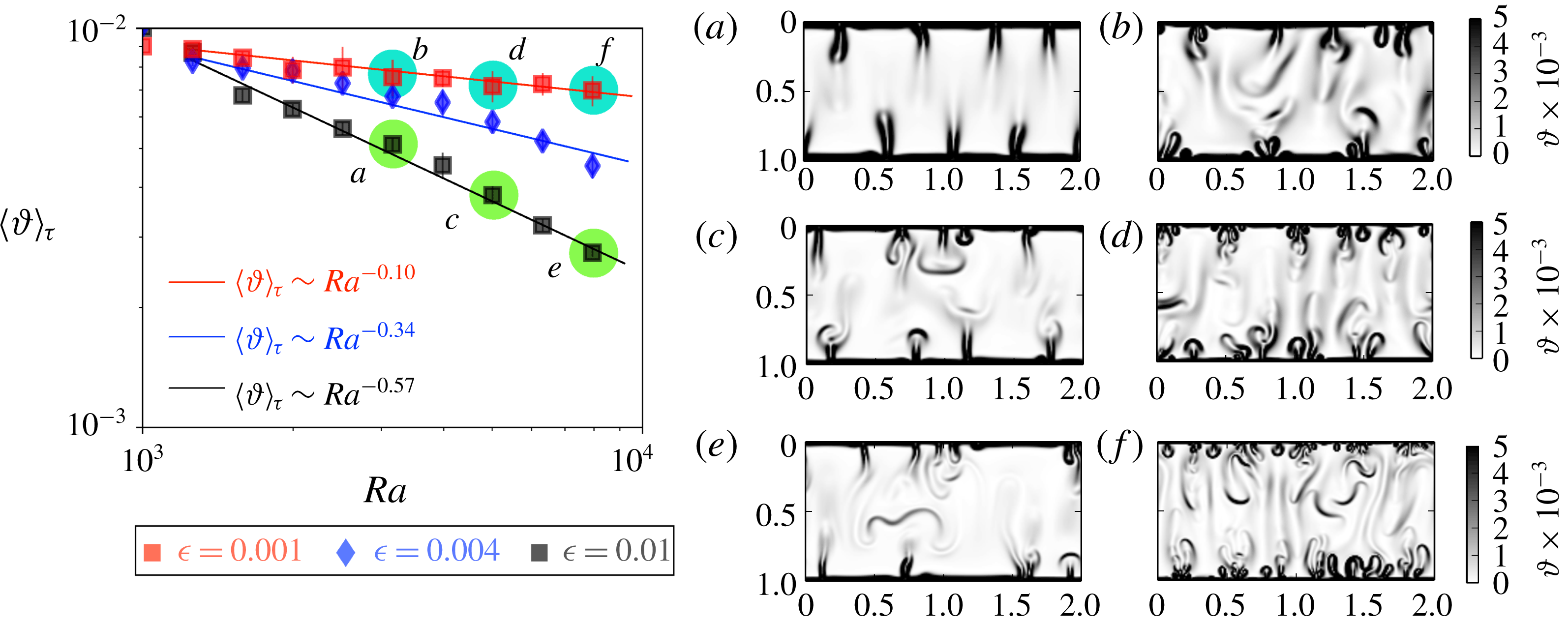
. In situations where dispersion is dominant, thermal dissipation can be unfavoured due to the homogenization of the temperature. This situation is displayed in figure 6, which shows regions that are actively mixed; these are effective shear zones identified as edges of thermal plumes. Plots (a,c,e) show cases where dispersion is dominant, presenting a low density of edges in contrast with plots (b,d,f), where dispersion is negligible and the Darcy drag term
 $\unicode[STIX]{x1D707}K^{-1}\boldsymbol{u}^{\ast }$
is dominant. For
 $\unicode[STIX]{x1D716}=0.001$
we have
 $\langle \unicode[STIX]{x1D717}\rangle _{\unicode[STIX]{x1D70F}}\sim Ra^{-0.10\pm 0.01}$
, which is not surprising since this case is similar to the porous media model prediction given indirectly by Hewitt et al. (Reference Hewitt, Neufeld and Lister2012), i.e. in the asymptotic case
 $\langle Nu\rangle _{\unicode[STIX]{x1D70F}}\sim Ra$
,
 $\langle \unicode[STIX]{x1D717}\rangle _{\unicode[STIX]{x1D70F}}$
is independent of
 $Ra$
. However, a new result is obtained for
 $\unicode[STIX]{x1D716}=0.004$
,
 $\langle \unicode[STIX]{x1D717}\rangle _{\unicode[STIX]{x1D70F}}\sim Ra^{-0.34\pm 0.03}$
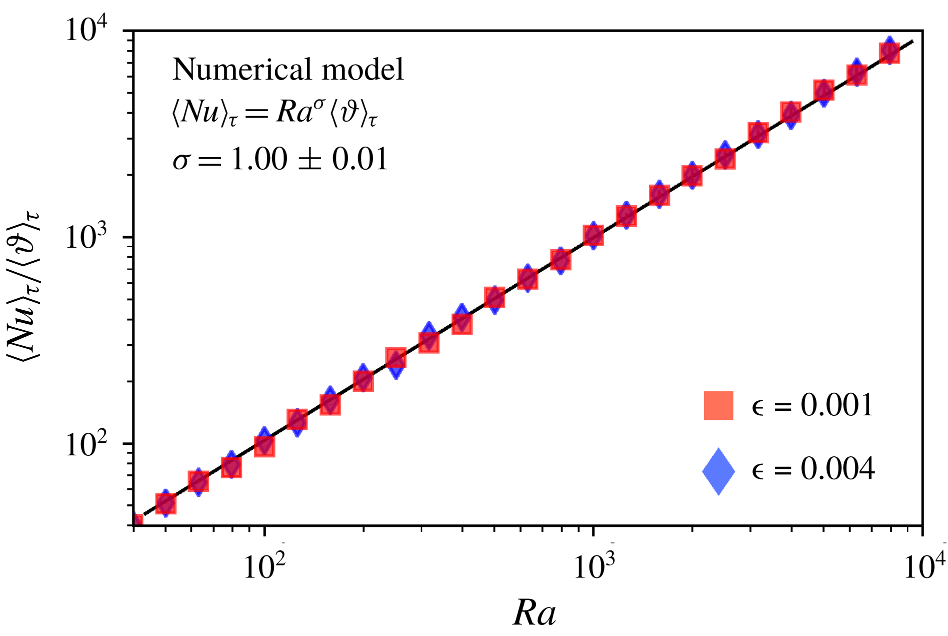
. Here, dispersive and inertial effects have consequences in the flow, allowing a better thermal homogenization. This result provides more conclusive evidence of the importance of perturbative corrections in thermal convection in Hele-Shaw cells. Finally, figure 7 shows that our numerical results are in good agreement with the theoretical prediction given in (3.13), so the effects of dispersion and inertial corrections are observed only in the exponents of the scalings
 $\langle Nu\rangle _{\unicode[STIX]{x1D70F}}\sim Ra^{\unicode[STIX]{x1D6FE}(\unicode[STIX]{x1D716})}$
and
 $\langle \unicode[STIX]{x1D717}\rangle _{\unicode[STIX]{x1D70F}}\sim Ra^{\unicode[STIX]{x1D6FE}(\unicode[STIX]{x1D716})-1}$
for the high-
 $Ra$
regime.
Parameter
 $\langle Nu\rangle _{\unicode[STIX]{x1D70F}}$
versus
 $\langle \unicode[STIX]{x1D717}\rangle _{\unicode[STIX]{x1D70F}}$
for all
 $\unicode[STIX]{x1D716}$
, which satisfy the theoretical relation
 $\langle Nu\rangle _{\unicode[STIX]{x1D70F}}=Ra\langle \unicode[STIX]{x1D717}\rangle _{\unicode[STIX]{x1D70F}}$
.

To derive a model for the exponent
 $\unicode[STIX]{x1D6FE}$
as a function of
 $\unicode[STIX]{x1D716}$
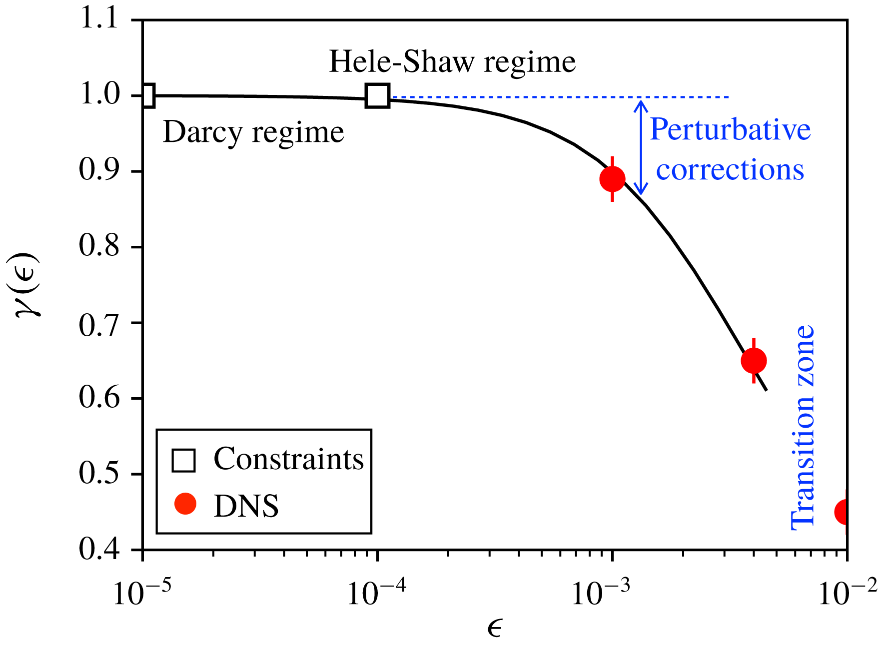
, we consider two regimes: (a) the Darcy regime, where
 $\unicode[STIX]{x1D716}\rightarrow 0$
, and (b) the Hele-Shaw regime, where
 $\unicode[STIX]{x1D716}$
is small and
 $\unicode[STIX]{x1D716}^{2}Ra\ll 1$
(see figure 8). In the Darcy regime, we assume
 $\unicode[STIX]{x1D6FE}=1$
. This constraint was inferred numerically by Hewitt et al. (Reference Hewitt, Neufeld and Lister2012) for
 $Ra>10^{5}$
, the ultimate regime for thermal convection in porous media. For the Hele-Shaw regime, we use the values of
 $\unicode[STIX]{x1D6FE}$
found by our numerical simulations. Therefore,
 $\unicode[STIX]{x1D6FE}(\unicode[STIX]{x1D716})$
can be estimated through the formula
 $$\begin{eqnarray}\displaystyle \unicode[STIX]{x1D6FE}(\unicode[STIX]{x1D716})=0.66-0.34\tanh [1.56\log _{10}(\unicode[STIX]{x1D716})+3.82], & & \displaystyle\end{eqnarray}$$
which quantifies the decrease of heat transport in Hele-Shaw geometries. Equation (4.3) is valid for the high-
 $Ra$
regime, i.e.
 $Ra>10^{3}$
, and
 $\unicode[STIX]{x1D716}^{2}Ra\ll 1$
. For example, if
 $\unicode[STIX]{x1D716}=10^{-3}$
, then
 $10^{3}<Ra\ll 10^{6}$
. In this case,
 $\langle Nu\rangle _{\unicode[STIX]{x1D70F}}\sim Ra^{0.90}$
. However, for
 $\unicode[STIX]{x1D716}=10^{-1}$
, this model is no longer valid because
 $Ra\ll 10^{2}$
. For
 $\unicode[STIX]{x1D716}^{2}Ra\sim O(1)$
, the problem becomes the 3D Rayleigh–Bénard convection (see figure 5).
In the literature, there are some interesting results concerning the values for the exponent
 $\unicode[STIX]{x1D6FE}$
in Rayleigh–Bénard convection. Waleffe, Boonkasane & Smith (Reference Waleffe, Boonkasane and Smith2015) show that heat flux becomes independent of the height as
 $Ra$
is very large. By using arguments of dimensional analysis, heat transport is determined by the marginal stability of the thermal boundary layers and mean temperature gradient (Malkus Reference Malkus1954), so the scaling proposed for this case is
 $\langle Nu\rangle _{\unicode[STIX]{x1D70F}}\sim Ra^{1/3}$
. However, Grossmann & Lohse (Reference Grossmann and Lohse2011) did a detailed interpretation of the experimental data reported by Ahlers, Funfschilling & Bodenschatz (Reference Ahlers, Funfschilling and Bodenschatz2009) for
 $Ra>10^{11}$
, showing that
 $\unicode[STIX]{x1D6FE}$
can vary from
 $0.14$
to
 $0.38$
, depending on the following heat transport features: (a) plume dominated, (b) dominated by the background thermal fluctuations or (c) thermal boundary layer is fully turbulent. The final state and scaling properties depend on the initial conditions or random fluctuations. It is interesting to note that
 $\unicode[STIX]{x1D6FE}$
values in Rayleigh–Bénard convection are lower than the values obtained for Darcy and Hele-Shaw regimes. Presumably,
 $\unicode[STIX]{x1D6FE}$
decreases from the Darcy and Hele-Shaw regimes towards the set of values found for Rayleigh–Bénard convection.
Equation (4.3) can be used to understand the aperture variability effects in vertical geological fractures. Variability effects appear explicitly in the permeability of the fracture, because
 $K$
depends on the aperture. With the aim of giving some orders of magnitude, we assume the fracture permeability as
 $K=b^{2}/12$
, where
 $b$
is the fracture aperture. At the field scale, for
 $b=1~\text{cm}$
, we obtain
 $K\sim 1\times 10^{-5}~\text{m}^{2}$
. If the fracture height is
 $H=10~\text{m}$
, the anisotropy ratio is
 $\unicode[STIX]{x1D716}\sim 3\times 10^{-4}$
. On the other hand, if
 $H=100~\text{m}$
,
 $\unicode[STIX]{x1D716}\sim 3\times 10^{-5}$
. For both cases, the Darcy regime is dominant and heat transport is optimized. However, for
 $b=10~\text{cm}$
and
 $H=10~\text{m}$
, we obtain
 $\unicode[STIX]{x1D716}\sim 3\times 10^{-3}$
. For the same aperture and
 $H=100~\text{m}$
,
 $\unicode[STIX]{x1D716}\sim 3\times 10^{-4}$
. Both cases are in the Hele-Shaw regime and heat transport is affected by the perturbative corrections of the porous media model.
Model for the exponent
 $\unicode[STIX]{x1D6FE}(\unicode[STIX]{x1D716})$
in the high-
 $Ra$
regime, valid for
 $\unicode[STIX]{x1D716}$
small and
 $\unicode[STIX]{x1D716}^{2}Ra\ll 1$
.

When the fracture aperture is narrowing, e.g. from
 $b=10~\text{cm}$
to
 $b=1~\text{cm}$
, flow channelling appears and the Darcy drag term starts to be dominant. Narrow apertures reduce the effects of longitudinal dispersion (transversal dispersion does not appear in Hele-Shaw flows) because mechanical dispersion is modulated by the square of the cell anisotropy ratio, as is shown in (3.6), so thermal dissipation is enhanced, creating columnar plumes. In this case, heat transport is efficient because fluid parcels can travel from hot zones to cold regions without losing energy. On the other hand, if the fracture aperture is widening, e.g. from
 $b=1~\text{cm}$
to
 $b=10~\text{cm}$
, thermal mixing is enhanced along the gap and heat transport is reduced, because a thermal parcel can exchange energy more efficiently with the surrounding fluid parcels.
Geological boundary conditions assume heat exchange between fluids and rocks at the fracture lateral walls. The incorporation of inhomogeneous Neumann boundary conditions modifies the critical
 $Ra$
for the onset of convection in fractures (Murphy Reference Murphy1979), but any change in the scaling properties of heat transport due to heat exchange has not been investigated so far. Thus, a future work related to this research is to study the consequences of including heat exchange boundary conditions at the fracture walls in the scaling laws
 $\langle Nu\rangle _{\unicode[STIX]{x1D70F}}=Ra^{\unicode[STIX]{x1D6FE}(\unicode[STIX]{x1D716})}$
and
 $\langle \unicode[STIX]{x1D717}\rangle _{\unicode[STIX]{x1D70F}}=Ra^{\unicode[STIX]{x1D6FE}(\unicode[STIX]{x1D716})-1}$
obtained by this work.
5 Conclusions
In this work, we have derived a 2D model that describes thermal convection in a Hele-Shaw cell, which is a laboratory representation of a vertical geological fracture heated from below and above. These equations are an extension of the porous media model, because they consider perturbative corrections given by the aperture of the cell. The equations include the effects of inertial corrections in the momentum equation and mechanical dispersion in the scalar equation. The introduction of the dimensionless parameters
 $\unicode[STIX]{x1D716}=\sqrt{K}/H$
and
 $Ra=\unicode[STIX]{x1D6FC}\unicode[STIX]{x0394}TgKH/\unicode[STIX]{x1D705}\unicode[STIX]{x1D707}$
allows one to characterize the problem. The response of the system is studied through the global Nusselt number
 $\langle Nu\rangle _{\unicode[STIX]{x1D70F}}$
. The application of our 2D model for a Hele-Shaw geometry, heated from below and above, leads to the following results and conclusions:
(1) For
 $\unicode[STIX]{x1D716}\geqslant 10^{-2}$
and
$4\unicode[STIX]{x03C0}^{2}\leqslant Ra<1000$
, the effects of the perturbative corrections do not change the scaling properties of
$\langle Nu\rangle _{\unicode[STIX]{x1D70F}}$
reported by Palm et al. (Reference Palm, Weber and Kvernvold1972), Otero et al. (Reference Otero, Dontcheva, Johnston, Worthing, Kurganov, Petrova and Doering2004) and Hewitt et al. (Reference Hewitt, Neufeld and Lister2012). This result was also reported by Kvernvold & Tyvand (Reference Kvernvold and Tyvand1981).
(2) The perturbative corrections start to be important for
$Ra>1350$
, the high-
$Ra$
regime, where new scalings for
$\langle Nu\rangle _{\unicode[STIX]{x1D70F}}$
are computed. This is the main contribution of this work. For
$\unicode[STIX]{x1D716}=0.001$
, we obtain
$\langle Nu\rangle _{\unicode[STIX]{x1D70F}}\sim Ra^{0.89}$
, but for
$\unicode[STIX]{x1D716}=0.004$
, we have
$\langle Nu\rangle _{\unicode[STIX]{x1D70F}}\sim Ra^{0.65}$
. Therefore, the scaling for heat transport is given by
$\langle Nu\rangle _{\unicode[STIX]{x1D70F}}\sim Ra^{\unicode[STIX]{x1D6FE}(\unicode[STIX]{x1D716})}$
, which is valid for
$\unicode[STIX]{x1D716}$
small and
$\unicode[STIX]{x1D716}^{2}Ra\ll 1$
.(3) The total thermal dissipation rate
$\langle \unicode[STIX]{x1D717}\rangle _{\unicode[STIX]{x1D70F}}$
scales as
$\langle \unicode[STIX]{x1D717}\rangle _{\unicode[STIX]{x1D70F}}\sim Ra^{\unicode[STIX]{x1D6FE}(\unicode[STIX]{x1D716})-1}$
in the high-
$Ra$
regime, which represents a new result for the problem. In the ultimate regime of thermal convection in porous media,
$\langle \unicode[STIX]{x1D717}\rangle _{\unicode[STIX]{x1D70F}}$
does not scale with
$Ra$
, which is a result obtained by Jenny et al. (Reference Jenny, Lee, Meyer and Tchelepi2014) in the context of mass transport.(4) We show theoretically and numerically that for Hele-Shaw cells
$\langle Nu\rangle _{\unicode[STIX]{x1D70F}}=Ra\langle \unicode[STIX]{x1D717}\rangle _{\unicode[STIX]{x1D70F}}$
, which is valid for
$Ra\geqslant 4\unicode[STIX]{x03C0}^{2}$
. For thermal convection in porous media,
$\langle Nu\rangle _{\unicode[STIX]{x1D70F}}=Ra$
in the ultimate regime (Hewitt et al.
Reference Hewitt, Neufeld and Lister2012).




The physics of the porous media scaling in the ultimate regime is very different from the multiple scaling found in Rayleigh–Bénard convection. The porous media convection supports columnar plumes that enhance heat transport, which is given by a unique scaling law,
 $\langle Nu\rangle _{\unicode[STIX]{x1D70F}}=Ra$
(Hewitt et al.
Reference Hewitt, Neufeld and Lister2012). On the other hand, the full 3D Rayleigh–Bénard problem is strongly affected by turbulent conditions at the kinetic boundary layer, reducing heat transport (Grossmann & Lohse Reference Grossmann and Lohse2011). The final state of Rayleigh–Bénard convection in the ultimate regime depends on the initial conditions or random fluctuations, so the scaling found by Grossmann & Lohse (Reference Grossmann and Lohse2011) varies from
 $\langle Nu\rangle _{\unicode[STIX]{x1D70F}}\sim Ra^{0.14}$
to
 $\langle Nu\rangle _{\unicode[STIX]{x1D70F}}\sim Ra^{0.38}$
. In the Hele-Shaw regime, the cell gap effects, captured by the longitudinal dispersion and inertial corrections, enhance thermal mixing processes and they introduce corrections into the scaling
 $\langle Nu\rangle _{\unicode[STIX]{x1D70F}}=Ra^{\unicode[STIX]{x1D6FE}(\unicode[STIX]{x1D716})}$
, reducing heat transport from
 $\unicode[STIX]{x1D6FE}=1$
presumably towards the values reported for Rayleigh–Bénard convection.
Acknowledgements
This work is a contribution from the FONDAP-CONICYT no. 15090013 project ‘Centro de Excelencia en Geotermia de los Andes (CEGA)’. J.A.L. acknowledges support from CONICYT through the National PhD Fellowship no. 21110836. The project CONICYT-PIA ‘Concurso apoyo a centros científicos y tecnológicos de excelencia con financiamiento basal’ AFB170001 CMM-UMI 2807 CNRS is also acknowledged. This research was partially supported by the supercomputing infrastructure of the National Laboratory High Performance Computing NLHPC (ECM-02).
Appendix A. Two-dimensional Hele-Shaw equations
The 2D set of equations (2.1)–(2.3) are derived from the full 3D model as follows. We consider a vertical Hele-Shaw cell heated from below and above at temperatures
 $T_{h}$
and
 $T_{c}$
, filled with a working fluid of constant viscosity
 $\unicode[STIX]{x1D707}$
and thermal diffusivity
 $\unicode[STIX]{x1D705}$
, and variable density
 $\unicode[STIX]{x1D70C}^{\ast }=\unicode[STIX]{x1D70C}_{c}-\unicode[STIX]{x1D6FC}(T^{\ast }-T_{c})$
, where
 $T^{\ast }$
is the temperature,
 $\unicode[STIX]{x1D6FC}$
is the thermal expansion coeficient and
 $\unicode[STIX]{x1D70C}_{c}$
is the density at the temperature
 $T_{c}$
(see figure 1). The fluid motion in this geometry under forced thermal convection is described by the incompressible Navier–Stokes and heat equations
 $$\begin{eqnarray}\displaystyle & \displaystyle \unicode[STIX]{x1D6FB}^{\ast }\boldsymbol{\cdot }\boldsymbol{v}^{\ast }=0, & \displaystyle\end{eqnarray}$$
 $$\begin{eqnarray}\displaystyle & \displaystyle \unicode[STIX]{x1D70C}_{c}\left(\frac{\unicode[STIX]{x2202}^{}{\boldsymbol{v}^{\ast }}_{}}{\unicode[STIX]{x2202}{t^{\ast }}^{}}+(\boldsymbol{v}^{\ast }\boldsymbol{\cdot }\unicode[STIX]{x1D6FB}^{\ast })\boldsymbol{v}^{\ast }\right)=-\unicode[STIX]{x1D6FB}^{\ast }\tilde{p}^{\ast }+\unicode[STIX]{x1D6FC}(T^{\ast }-T_{c})g\hat{z}+\unicode[STIX]{x1D707}\unicode[STIX]{x1D6FB}^{\ast 2}\boldsymbol{v}^{\ast }, & \displaystyle\end{eqnarray}$$
 $$\begin{eqnarray}\displaystyle & \displaystyle \frac{\unicode[STIX]{x2202}^{}{T^{\ast }}_{}}{\unicode[STIX]{x2202}{t^{\ast }}^{}}+(\boldsymbol{v}^{\ast }\boldsymbol{\cdot }\unicode[STIX]{x1D6FB}^{\ast })T^{\ast }=\unicode[STIX]{x1D705}\unicode[STIX]{x1D6FB}^{\ast 2}T^{\ast }. & \displaystyle\end{eqnarray}$$
In the above equations,
 $\boldsymbol{v}^{\ast }=u^{\ast }\hat{x}+v^{\ast }{\hat{y}}+w^{\ast }\hat{z}$
is the velocity field,
 $\tilde{p}^{\ast }=p^{\ast }+\unicode[STIX]{x1D70C}_{c}gz^{\ast }$
is the modified pressure and
 $g$
is the gravitational acceleration. The boundary conditions are periodic in
 $x$
-axis,
 $u^{\ast }=0$
,
 $v^{\ast }=0$
,
 $w^{\ast }=0$
,
 $\unicode[STIX]{x2202}T^{\ast }/\unicode[STIX]{x2202}y^{\ast }=0$
at
 $y^{\ast }=0$
and
 $y^{\ast }=b$
,
 $\unicode[STIX]{x2202}u^{\ast }/\unicode[STIX]{x2202}z^{\ast }=0$
,
 $v^{\ast }=0$
,
 $w^{\ast }=0$
at
 $z^{\ast }=0$
and
 $z^{\ast }=H$
,
 $T^{\ast }=T_{h}$
at
 $z^{\ast }=0$
and
 $T^{\ast }=T_{c}$
at
 $z^{\ast }=H$
. Equations (A 1)–(A 3) constitute the problem to be solved.
To adimensionalize (A 1)–(A 3), we use the following variables for positions
 $x^{\prime }=x^{\ast }/H$
,
 $y^{\prime }=y^{\ast }/b$
and
 $z^{\prime }=z^{\ast }/H$
, velocity
 $\boldsymbol{v}^{\prime }=\boldsymbol{v}^{\ast }/v_{c}$
, time
 $t^{\prime }=v_{c}t^{\ast }/H$
, pressure
 $p^{\prime }=\tilde{p}^{\ast }/p_{s}$
and temperature
 $T^{\prime }=(T^{\ast }-T_{c})/(T_{h}-T_{c})$
, where
 $v_{c}=\unicode[STIX]{x1D6FC}(T_{h}-T_{c})gb^{2}/\unicode[STIX]{x1D707}$
is the characteristic velocity and
 $p_{s}=\unicode[STIX]{x1D707}v_{c}H/b^{2}$
is the characteristic pressure. This dimensionless scheme has been used in convection problems in porous media (Otero et al.
Reference Otero, Dontcheva, Johnston, Worthing, Kurganov, Petrova and Doering2004; Riaz et al.
Reference Riaz, Hesse, Tchelepi and Orr2006). The dimensionless equations are written in terms of two parameters, the Prandtl number
 $Pr=\unicode[STIX]{x1D708}/\unicode[STIX]{x1D705}$
and the Rayleigh number
 $Ra=v_{c}H/\unicode[STIX]{x1D705}$
, where
 $\unicode[STIX]{x1D708}=\unicode[STIX]{x1D707}/\unicode[STIX]{x1D70C}_{c}$
is the kinematic viscosity at the temperature
 $T^{\ast }=T_{c}$
. Finally, to reduce the 3D formulation of the problem to a 2D set of equations, we introduce the small parameter
 $\unicode[STIX]{x1D6FF}=b/H\ll 1$
, which measures the ratio of cell spacing to height.
It is important to notice that the perturbative parameter used in this appendix is
 $\unicode[STIX]{x1D6FF}=b/H$
. However, in the main text, the perturbative parameter used is
 $\unicode[STIX]{x1D716}=\sqrt{K}/H$
, where
 $K=b^{2}/12$
is the cell permeability. Therefore,
 $\unicode[STIX]{x1D716}^{2}=\unicode[STIX]{x1D6FF}^{2}/12$
. The same fact occurs with the velocity scale, where the relation is
 $u_{c}=v_{c}/12$
, and the dimensionless definitions for time, pressure and Rayleigh number given in this appendix.
The dimensionless form of (A 1) and the vertical component of (A 2) are
 $$\begin{eqnarray}\displaystyle & \displaystyle \unicode[STIX]{x1D6FF}\left(\frac{\unicode[STIX]{x2202}u^{\prime }}{\unicode[STIX]{x2202}x^{\prime }}+\frac{\unicode[STIX]{x2202}w^{\prime }}{\unicode[STIX]{x2202}z^{\prime }}\right)+\frac{\unicode[STIX]{x2202}v^{\prime }}{\unicode[STIX]{x2202}y^{\prime }}=0, & \displaystyle\end{eqnarray}$$
 $$\begin{eqnarray}\displaystyle & \displaystyle \unicode[STIX]{x1D6FF}\frac{Ra}{Pr}\left[\unicode[STIX]{x1D6FF}\left(\frac{\unicode[STIX]{x2202}w^{\prime }}{\unicode[STIX]{x2202}t^{\prime }}+u^{\prime }\frac{\unicode[STIX]{x2202}w^{\prime }}{\unicode[STIX]{x2202}x^{\prime }}+w^{\prime }\frac{\unicode[STIX]{x2202}w^{\prime }}{\unicode[STIX]{x2202}z^{\prime }}\right)+v^{\prime }\frac{\unicode[STIX]{x2202}w^{\prime }}{\unicode[STIX]{x2202}y^{\prime }}\right]=-\frac{\unicode[STIX]{x2202}p^{\prime }}{\unicode[STIX]{x2202}z^{\prime }}+T^{\prime }+\unicode[STIX]{x1D6FF}^{2}\left(\frac{\unicode[STIX]{x2202}^{2}w^{\prime }}{\unicode[STIX]{x2202}x^{\prime 2}}+\frac{\unicode[STIX]{x2202}^{2}w^{\prime }}{\unicode[STIX]{x2202}z^{\prime 2}}\right)+\frac{\unicode[STIX]{x2202}^{2}w^{\prime }}{\unicode[STIX]{x2202}y^{\prime 2}}. & \displaystyle \nonumber\\ \displaystyle & & \displaystyle\end{eqnarray}$$
A comparison of the orders of magnitude of all variables in the above equations leads to the following scaling relations:
 $$\begin{eqnarray}\displaystyle \frac{\unicode[STIX]{x2202}p^{\prime }}{\unicode[STIX]{x2202}z^{\prime }}\sim \frac{\unicode[STIX]{x2202}^{2}w^{\prime }}{\unicode[STIX]{x2202}y^{\prime 2}}\sim T^{\prime };\quad \unicode[STIX]{x1D6FF}^{2}\frac{\unicode[STIX]{x2202}w^{\prime }}{\unicode[STIX]{x2202}t^{\prime }}\sim \unicode[STIX]{x1D6FF}^{2}\frac{\unicode[STIX]{x2202}^{2}w^{\prime }}{\unicode[STIX]{x2202}z^{\prime 2}};\quad \unicode[STIX]{x1D6FF}\frac{\unicode[STIX]{x2202}w^{\prime }}{\unicode[STIX]{x2202}z^{\prime }}\sim \frac{\unicode[STIX]{x2202}v^{\prime }}{\unicode[STIX]{x2202}y^{\prime }}. & & \displaystyle\end{eqnarray}$$
Since
 $y^{\prime }\sim O(1)$
,
 $z^{\prime }\sim O(1)$
and
 $T^{\prime }\sim O(1)$
, we obtain
 $t^{\prime }\sim O(1)$
,
 $v^{\prime }\sim O(\unicode[STIX]{x1D6FF})$
,
 $w^{\prime }\sim O(1)$
and
 $p^{\prime }\sim O(1)$
. Therefore, we define the following scalings:
 $x^{\prime }=x$
,
 $y^{\prime }=y$
,
 $z^{\prime }=z$
,
 $u^{\prime }=u$
,
 $v^{\prime }=\unicode[STIX]{x1D6FF}v$
,
 $w^{\prime }=w$
,
 $t^{\prime }=t$
,
 $p=p^{\prime }$
and
 $T^{\prime }=T$
. Assuming
 $Pr>1$
,
 $\unicode[STIX]{x1D6FF}\ll 1$
and
 $\unicode[STIX]{x1D6FF}^{2}Ra\ll 1$
, the equations are written as
 $$\begin{eqnarray}\displaystyle & \displaystyle \frac{\unicode[STIX]{x2202}^{}u_{}}{\unicode[STIX]{x2202}x^{}}+\frac{\unicode[STIX]{x2202}^{}v_{}}{\unicode[STIX]{x2202}y^{}}+\frac{\unicode[STIX]{x2202}^{}w_{}}{\unicode[STIX]{x2202}z^{}}=0, & \displaystyle\end{eqnarray}$$
 $$\begin{eqnarray}\displaystyle & \displaystyle \unicode[STIX]{x1D6FF}^{2}\frac{Ra}{Pr}\left(\frac{\unicode[STIX]{x2202}^{}u_{}}{\unicode[STIX]{x2202}y^{}}+u\frac{\unicode[STIX]{x2202}^{}u_{}}{\unicode[STIX]{x2202}x^{}}+v\frac{\unicode[STIX]{x2202}^{}u_{}}{\unicode[STIX]{x2202}y^{}}+w\frac{\unicode[STIX]{x2202}^{}u_{}}{\unicode[STIX]{x2202}z^{}}\right)=-\frac{\unicode[STIX]{x2202}^{}p_{}}{\unicode[STIX]{x2202}x^{}}+\frac{\unicode[STIX]{x2202}^{2}u_{}}{\unicode[STIX]{x2202}y^{2}}+\unicode[STIX]{x1D6FF}^{2}\left(\frac{\unicode[STIX]{x2202}^{2}u_{}}{\unicode[STIX]{x2202}x^{2}}+\frac{\unicode[STIX]{x2202}^{2}u_{}}{\unicode[STIX]{x2202}z^{2}}\right), & \displaystyle\end{eqnarray}$$
 $$\begin{eqnarray}\displaystyle & \displaystyle \unicode[STIX]{x1D6FF}^{4}\frac{Ra}{Pr}\left(\frac{\unicode[STIX]{x2202}^{}v_{}}{\unicode[STIX]{x2202}t^{}}+u\frac{\unicode[STIX]{x2202}^{}v_{}}{\unicode[STIX]{x2202}x^{}}+v\frac{\unicode[STIX]{x2202}^{}v_{}}{\unicode[STIX]{x2202}y^{}}+w\frac{\unicode[STIX]{x2202}^{}v_{}}{\unicode[STIX]{x2202}z^{}}\right)=-\frac{\unicode[STIX]{x2202}^{}p_{}}{\unicode[STIX]{x2202}y^{}}+\unicode[STIX]{x1D6FF}^{2}\frac{\unicode[STIX]{x2202}^{2}v_{}}{\unicode[STIX]{x2202}y^{2}}+\unicode[STIX]{x1D6FF}^{4}\left(\frac{\unicode[STIX]{x2202}^{2}v_{}}{\unicode[STIX]{x2202}x^{2}}+\frac{\unicode[STIX]{x2202}^{2}v_{}}{\unicode[STIX]{x2202}z^{2}}\right), & \displaystyle\end{eqnarray}$$
 $$\begin{eqnarray}\displaystyle & \displaystyle \unicode[STIX]{x1D6FF}^{2}\frac{Ra}{Pr}\left(\frac{\unicode[STIX]{x2202}^{}w_{}}{\unicode[STIX]{x2202}y^{}}+u\frac{\unicode[STIX]{x2202}^{}w_{}}{\unicode[STIX]{x2202}x^{}}+v\frac{\unicode[STIX]{x2202}^{}w_{}}{\unicode[STIX]{x2202}y^{}}+w\frac{\unicode[STIX]{x2202}^{}w_{}}{\unicode[STIX]{x2202}z^{}}\right)=-\frac{\unicode[STIX]{x2202}^{}p_{}}{\unicode[STIX]{x2202}z^{}}+T+\frac{\unicode[STIX]{x2202}^{2}w_{}}{\unicode[STIX]{x2202}y^{2}}+\unicode[STIX]{x1D6FF}^{2}\left(\frac{\unicode[STIX]{x2202}^{2}w_{}}{\unicode[STIX]{x2202}x^{2}}+\frac{\unicode[STIX]{x2202}^{2}w_{}}{\unicode[STIX]{x2202}z^{2}}\right),\qquad & \displaystyle\end{eqnarray}$$
 $$\begin{eqnarray}\displaystyle & \displaystyle \unicode[STIX]{x1D6FF}^{2}Ra\left(\frac{\unicode[STIX]{x2202}^{}T_{}}{\unicode[STIX]{x2202}t^{}}+u\frac{\unicode[STIX]{x2202}^{}T_{}}{\unicode[STIX]{x2202}x^{}}+v\frac{\unicode[STIX]{x2202}^{}T_{}}{\unicode[STIX]{x2202}y^{}}+w\frac{\unicode[STIX]{x2202}^{}T_{}}{\unicode[STIX]{x2202}z^{}}\right)=\unicode[STIX]{x1D6FF}^{2}\left(\frac{\unicode[STIX]{x2202}^{2}T_{}}{\unicode[STIX]{x2202}x^{2}}+\frac{\unicode[STIX]{x2202}^{2}T_{}}{\unicode[STIX]{x2202}z^{2}}\right)+\frac{\unicode[STIX]{x2202}^{2}T_{}}{\unicode[STIX]{x2202}y^{2}}. & \displaystyle\end{eqnarray}$$
For
 $\unicode[STIX]{x1D6FF}=0$
, we obtain the Stokes model coupled with heat transport. It is well known that the solution of (A 7)–(A 9) for
 $\unicode[STIX]{x1D6FF}=0$
, with regards to variable
 $y$
, leads to the Darcy model. The relevant parameter in (A 7)–(A 11) is
 $\unicode[STIX]{x1D6FF}^{2}\ll 1$
, so the inertial corrections of the Darcy model are found solving perturbatively the dimensionless equations by expanding all physical variables as
 $f=f_{0}+\unicode[STIX]{x1D6FF}^{2}f_{1}+\unicode[STIX]{x1D6FF}^{4}f_{2}+O(\unicode[STIX]{x1D6FF}^{6})$
, where
 $f$
represents any of the dependent variables
 $u$
,
 $v$
,
 $w$
,
 $p$
,
 $T$
. With this procedure, we can obtain a more general model for Hele-Shaw flows.
A.1 Leading-order solutions
At the leading order, the equations to be solved are
 $$\begin{eqnarray}\displaystyle & \displaystyle \frac{\unicode[STIX]{x2202}^{}u_{0}}{\unicode[STIX]{x2202}x^{}}+\frac{\unicode[STIX]{x2202}^{}v_{0}}{\unicode[STIX]{x2202}y^{}}+\frac{\unicode[STIX]{x2202}^{}w_{0}}{\unicode[STIX]{x2202}z^{}}=0, & \displaystyle\end{eqnarray}$$
 $$\begin{eqnarray}\displaystyle & \displaystyle -\frac{\unicode[STIX]{x2202}^{}p_{0}}{\unicode[STIX]{x2202}x^{}}+\frac{\unicode[STIX]{x2202}^{2}u_{0}}{\unicode[STIX]{x2202}y^{2}}=0, & \displaystyle\end{eqnarray}$$
 $$\begin{eqnarray}\displaystyle & \displaystyle \frac{\unicode[STIX]{x2202}^{}p_{0}}{\unicode[STIX]{x2202}y^{}}=0, & \displaystyle\end{eqnarray}$$
 $$\begin{eqnarray}\displaystyle & \displaystyle -\frac{\unicode[STIX]{x2202}^{}p_{0}}{\unicode[STIX]{x2202}z^{}}+T_{0}+\frac{\unicode[STIX]{x2202}^{2}w_{0}}{\unicode[STIX]{x2202}y^{2}}=0, & \displaystyle\end{eqnarray}$$
 $$\begin{eqnarray}\displaystyle & \displaystyle \frac{\unicode[STIX]{x2202}^{2}T_{0}}{\unicode[STIX]{x2202}y^{2}}=0, & \displaystyle\end{eqnarray}$$
subject to the boundary conditions
 $u_{0}=0$
,
 $v_{0}=0$
,
 $w_{0}=0$
,
 $\unicode[STIX]{x2202}T_{0}/\unicode[STIX]{x2202}y=0$
at
 $y=0$
and
 $y=1$
. At order
 $O(1)$
, the solution of the transport equation (A 16) is
 $T_{0}=T_{0}(x,z,t)$
. From (A 14), the solution for the pressure is
 $p_{0}=p_{0}(x,z,t)$
and the velocities
 $u_{0}$
,
 $v_{0}$
and
 $w_{0}$
satisfy the Poiseuille flow
 $$\begin{eqnarray}\displaystyle \unicode[STIX]{x1D707}_{0}u_{0}=\frac{1}{2}\frac{\unicode[STIX]{x2202}^{}p_{0}}{\unicode[STIX]{x2202}x^{}}(y^{2}-y);\quad v_{0}=0;\quad \unicode[STIX]{x1D707}_{0}w_{0}=\frac{1}{2}\left(\frac{\unicode[STIX]{x2202}^{}p_{0}}{\unicode[STIX]{x2202}z^{}}-T_{0}\right)(y^{2}-y).\quad & & \displaystyle\end{eqnarray}$$
We define the mean value of
 $f(y)$
in the
 ${\hat{y}}$
(transverse) direction as
 $\bar{f}=\int _{0}^{1}f(y)\,\text{d}y$
. Applying this averaging process to (A 17), we obtain the 2D model
 $$\begin{eqnarray}\displaystyle \bar{u}_{0}^{}=-\frac{1}{12}\frac{\unicode[STIX]{x2202}^{}\bar{p}_{0}}{\unicode[STIX]{x2202}x^{}};\quad \bar{v}_{0}=0;\quad \bar{w}_{0}^{}=-\frac{1}{12}\left(\frac{\unicode[STIX]{x2202}^{}\bar{p}_{0}}{\unicode[STIX]{x2202}z^{}}-\bar{T}_{0}^{}\right). & & \displaystyle\end{eqnarray}$$
Equation (A 18) is the well-known Darcy equation or Hele-Shaw model at the leading order.
A.2
$O(\unicode[STIX]{x1D6FF}^{2})$
solutions

At order
 $O(\unicode[STIX]{x1D6FF}^{2})$
, the equations to be solved are
 $$\begin{eqnarray}\displaystyle & \displaystyle \frac{\unicode[STIX]{x2202}^{}u_{1}}{\unicode[STIX]{x2202}x^{}}+\frac{\unicode[STIX]{x2202}^{}v_{1}}{\unicode[STIX]{x2202}y^{}}+\frac{\unicode[STIX]{x2202}^{}w_{1}}{\unicode[STIX]{x2202}z^{}}=0, & \displaystyle\end{eqnarray}$$
 $$\begin{eqnarray}\displaystyle & \displaystyle \frac{Ra}{Pr}\left(\frac{\unicode[STIX]{x2202}^{}u_{0}}{\unicode[STIX]{x2202}y^{}}+u_{0}\frac{\unicode[STIX]{x2202}^{}u_{0}}{\unicode[STIX]{x2202}x^{}}+v_{0}\frac{\unicode[STIX]{x2202}^{}u_{0}}{\unicode[STIX]{x2202}y^{}}+w_{0}\frac{\unicode[STIX]{x2202}^{}u_{0}}{\unicode[STIX]{x2202}z^{}}\right)=-\frac{\unicode[STIX]{x2202}^{}p_{1}}{\unicode[STIX]{x2202}x^{}}+\frac{\unicode[STIX]{x2202}^{2}u_{1}}{\unicode[STIX]{x2202}y^{2}}+\frac{\unicode[STIX]{x2202}^{2}u_{0}}{\unicode[STIX]{x2202}x^{2}}+\frac{\unicode[STIX]{x2202}^{2}u_{0}}{\unicode[STIX]{x2202}z^{2}}, & \displaystyle\end{eqnarray}$$
 $$\begin{eqnarray}\displaystyle & \displaystyle -\frac{\unicode[STIX]{x2202}^{}p_{1}}{\unicode[STIX]{x2202}y^{}}+\frac{\unicode[STIX]{x2202}^{2}v_{0}}{\unicode[STIX]{x2202}y^{2}}=0, & \displaystyle\end{eqnarray}$$
 $$\begin{eqnarray}\displaystyle & \displaystyle \frac{Ra}{Pr}\left(\frac{\unicode[STIX]{x2202}^{}w_{0}}{\unicode[STIX]{x2202}y^{}}+u_{0}\frac{\unicode[STIX]{x2202}^{}w_{0}}{\unicode[STIX]{x2202}x^{}}+v_{0}\frac{\unicode[STIX]{x2202}^{}w_{0}}{\unicode[STIX]{x2202}y^{}}+w_{0}\frac{\unicode[STIX]{x2202}^{}w_{0}}{\unicode[STIX]{x2202}z^{}}\right)=-\frac{\unicode[STIX]{x2202}^{}p_{1}}{\unicode[STIX]{x2202}z^{}}+T_{1}+\frac{\unicode[STIX]{x2202}^{2}w_{1}}{\unicode[STIX]{x2202}y^{2}}+\frac{\unicode[STIX]{x2202}^{2}w_{0}}{\unicode[STIX]{x2202}x^{2}}+\frac{\unicode[STIX]{x2202}^{2}w_{0}}{\unicode[STIX]{x2202}z^{2}}, & \displaystyle \nonumber\\ \displaystyle & & \displaystyle\end{eqnarray}$$
 $$\begin{eqnarray}\displaystyle & \displaystyle Ra\left(\frac{\unicode[STIX]{x2202}^{}T_{0}}{\unicode[STIX]{x2202}t^{}}+u_{0}\frac{\unicode[STIX]{x2202}^{}T_{0}}{\unicode[STIX]{x2202}x^{}}+w_{0}\frac{\unicode[STIX]{x2202}^{}T_{0}}{\unicode[STIX]{x2202}z^{}}\right)=\frac{\unicode[STIX]{x2202}^{2}T_{0}}{\unicode[STIX]{x2202}x^{2}}+\frac{\unicode[STIX]{x2202}^{2}T_{0}}{\unicode[STIX]{x2202}z^{2}}+\frac{\unicode[STIX]{x2202}^{2}T_{1}}{\unicode[STIX]{x2202}y^{2}}, & \displaystyle\end{eqnarray}$$
subject to the boundary conditions
 $u_{1}=0$
,
 $v_{1}=0$
,
 $w_{1}=0$
,
 $\unicode[STIX]{x2202}T_{1}/\unicode[STIX]{x2202}y=0$
at
 $y=0$
and
 $y=1$
. Averaging (A 23) in the transverse direction and applying the above boundary conditions, we obtain the advection–diffusion equation for heat transport
 $$\begin{eqnarray}\displaystyle \frac{\unicode[STIX]{x2202}^{}\bar{T}_{0}}{\unicode[STIX]{x2202}t^{}}+\bar{u}_{0}\frac{\unicode[STIX]{x2202}^{}\bar{T}_{0}}{\unicode[STIX]{x2202}x^{}}+\bar{w}_{0}\frac{\unicode[STIX]{x2202}^{}\bar{T}_{0}}{\unicode[STIX]{x2202}z^{}}=\frac{1}{Ra}\left(\frac{\unicode[STIX]{x2202}^{2}\bar{T}_{0}}{\unicode[STIX]{x2202}x^{2}}+\frac{\unicode[STIX]{x2202}^{2}\bar{T}_{0}}{\unicode[STIX]{x2202}z^{2}}\right), & & \displaystyle\end{eqnarray}$$
which is the solubility condition at this order. The velocity, pressure and temperature satisfy the variable dependency
 $f=f(x,y,z,t)$
, where
 $f$
is any of the variables
 $u_{1}$
,
 $w_{1}$
,
 $T_{1}$
and
 $p_{1}$
. Considering
 $\boldsymbol{v}_{0}=u_{0}\hat{x}+w_{0}\hat{z}$
,
 $\boldsymbol{v}_{1}=u_{1}\hat{x}+w_{1}\hat{z}$
,
 $\unicode[STIX]{x1D735}_{\bot }=\unicode[STIX]{x2202}/\unicode[STIX]{x2202}x\hat{x}+\unicode[STIX]{x2202}/\unicode[STIX]{x2202}z\hat{z}$
and
 $h(y)=y(1-y)$
, explicit solutions for the temperature and velocity field at this order are
 $$\begin{eqnarray}\displaystyle T_{1}=\bar{T}_{1}-Ra(\bar{\boldsymbol{v}}_{0}\boldsymbol{\cdot }\unicode[STIX]{x1D735}_{\bot }\bar{T}_{0})\left(\frac{1}{2}h^{2}-\frac{1}{60}\right), & & \displaystyle\end{eqnarray}$$
 $$\begin{eqnarray}\displaystyle \boldsymbol{v}_{1} & = & \displaystyle 5\bar{\boldsymbol{v}}_{1}(h^{2}+h)-\frac{Ra}{Pr}(\bar{\boldsymbol{v}}_{0}\boldsymbol{\cdot }\unicode[STIX]{x1D735}_{\bot })\bar{\boldsymbol{v}}_{0}\left(\frac{6}{5}h^{3}-\frac{3}{70}h^{2}-\frac{3}{70}h\right)\nonumber\\ \displaystyle & & \displaystyle +\,(\unicode[STIX]{x1D735}_{\bot }\bar{p}_{1}-\bar{T}_{1}\hat{z})\left(\frac{5}{12}h^{2}-\frac{1}{12}h\right)-Ra(\bar{\boldsymbol{v}}_{0}\boldsymbol{\cdot }\unicode[STIX]{x1D735}_{\bot }\bar{T}_{0})\hat{z}\left(\frac{1}{60}h^{3}+\frac{2}{315}h^{2}-\frac{1}{504}h\right).\nonumber\\ \displaystyle & & \displaystyle\end{eqnarray}$$
Furthermore,
 $p_{1}=\bar{p}_{1}(x,z,t)$
. The averaged velocity
 $\bar{\boldsymbol{v}}_{1}$
satisfies the equation
 $$\begin{eqnarray}\displaystyle & \displaystyle 12\bar{\boldsymbol{v}}_{1}=-\unicode[STIX]{x1D735}_{\bot }\bar{p}_{1}+\left(\bar{T}_{1}-\frac{1}{210}Ra(\bar{\boldsymbol{v}}_{0}\boldsymbol{\cdot }\unicode[STIX]{x1D735}_{\bot }\bar{T}_{0})\right)\hat{z}-\frac{Ra}{Pr}\frac{{\mathcal{D}}\bar{\boldsymbol{v}}_{0}}{{\mathcal{D}}t}+\frac{6}{5}\unicode[STIX]{x1D6FB}_{\bot }^{2}\bar{\boldsymbol{v}}_{0}, & \displaystyle\end{eqnarray}$$
 $$\begin{eqnarray}\displaystyle & \displaystyle \frac{{\mathcal{D}}\bar{\boldsymbol{v}}_{0}}{{\mathcal{D}}t}=\frac{6}{5}\frac{\unicode[STIX]{x2202}^{}\bar{\boldsymbol{v}}_{0}}{\unicode[STIX]{x2202}t^{}}+\frac{54}{35}(\bar{\boldsymbol{v}}_{0}\boldsymbol{\cdot }\unicode[STIX]{x1D735}_{\bot })\bar{\boldsymbol{v}}_{0}, & \displaystyle\end{eqnarray}$$
which is an extension of the Darcy model.
A.3
$O(\unicode[STIX]{x1D6FF}^{4})$
solutions

The equation for the scalar transport is
 $$\begin{eqnarray}\displaystyle Ra\left(\frac{\unicode[STIX]{x2202}^{}T_{1}}{\unicode[STIX]{x2202}t^{}}+u_{0}\frac{\unicode[STIX]{x2202}^{}T_{1}}{\unicode[STIX]{x2202}x^{}}+u_{1}\frac{\unicode[STIX]{x2202}^{}T_{0}}{\unicode[STIX]{x2202}x^{}}+w_{0}\frac{\unicode[STIX]{x2202}^{}T_{1}}{\unicode[STIX]{x2202}z^{}}+w_{1}\frac{\unicode[STIX]{x2202}^{}T_{0}}{\unicode[STIX]{x2202}z^{}}\right)=\frac{\unicode[STIX]{x2202}^{2}T_{1}}{\unicode[STIX]{x2202}x^{2}}+\frac{\unicode[STIX]{x2202}^{2}T_{1}}{\unicode[STIX]{x2202}z^{2}}+\frac{\unicode[STIX]{x2202}^{2}T_{2}}{\unicode[STIX]{x2202}y^{2}}, & & \displaystyle\end{eqnarray}$$
subject to the boundary condition
 $\unicode[STIX]{x2202}T_{2}/\unicode[STIX]{x2202}y=0$
at
 $y=0$
and
 $y=1$
. Using the same average process described in this appendix, we obtain the advection–diffusion equation with the mechanical thermal dispersion
 ${\mathcal{D}}_{mec}^{(0)}$
for Hele-Shaw geometries
 $$\begin{eqnarray}\displaystyle & \displaystyle \frac{\unicode[STIX]{x2202}^{}\bar{T}_{1}}{\unicode[STIX]{x2202}t^{}}+\bar{u}_{0}\frac{\unicode[STIX]{x2202}^{}\bar{T}_{1}}{\unicode[STIX]{x2202}x^{}}+\bar{u}_{1}\frac{\unicode[STIX]{x2202}^{}\bar{T}_{0}}{\unicode[STIX]{x2202}x^{}}+\bar{w}_{0}\frac{\unicode[STIX]{x2202}^{}\bar{T}_{1}}{\unicode[STIX]{x2202}z^{}}+\bar{w}_{1}\frac{\unicode[STIX]{x2202}^{}\bar{T}_{0}}{\unicode[STIX]{x2202}z^{}}=\frac{1}{Ra}\left(\frac{\unicode[STIX]{x2202}^{2}\bar{T}_{1}}{\unicode[STIX]{x2202}x^{2}}+\frac{\unicode[STIX]{x2202}^{2}\bar{T}_{1}}{\unicode[STIX]{x2202}z^{2}}\right)+{\mathcal{D}}_{mec}^{(0)},\quad & \displaystyle\end{eqnarray}$$
 $$\begin{eqnarray}\displaystyle & \displaystyle {\mathcal{D}}_{mec}^{(0)}=\frac{Ra}{210}\left[\bar{u}_{0}\frac{\unicode[STIX]{x2202}}{\unicode[STIX]{x2202}x}\left(\bar{u}_{0}\frac{\unicode[STIX]{x2202}^{}\bar{T}_{0}}{\unicode[STIX]{x2202}x^{}}+\bar{w}_{0}\frac{\unicode[STIX]{x2202}^{}\bar{T}_{0}}{\unicode[STIX]{x2202}z^{}}\right)+\bar{w}_{0}\frac{\unicode[STIX]{x2202}}{\unicode[STIX]{x2202}z}\left(\bar{u}_{0}\frac{\unicode[STIX]{x2202}^{}\bar{T}_{0}}{\unicode[STIX]{x2202}x^{}}+\bar{w}_{0}\frac{\unicode[STIX]{x2202}^{}\bar{T}_{0}}{\unicode[STIX]{x2202}z^{}}\right)\right], & \displaystyle\end{eqnarray}$$
which is the solubility condition at this order. Equation (A 30) is important because thermal dispersion and inertial corrections in momentum equations appear at the same order.
A.4 The Hele-Shaw model
Using the corrections shown above, a general equation is constructed using
 $\bar{\boldsymbol{v}}=(\bar{u}_{0}+\unicode[STIX]{x1D6FF}^{2}\bar{u}_{1})\hat{x}+(\bar{w}_{0}+\unicode[STIX]{x1D6FF}^{2}\bar{w}_{1})\hat{z}$
,
 $\bar{T}=\bar{T}_{0}+\unicode[STIX]{x1D6FF}^{2}\bar{T}_{1}$
and
 $\bar{p}=\bar{p}_{0}+\unicode[STIX]{x1D6FF}^{2}\bar{p}_{1}$
, where
 $\bar{f}=\int _{0}^{1}f(y)\,\text{d}y$
is any of the dependent variables
 $\bar{u}$
,
 $\bar{w}$
,
 $\bar{p}$
and
 $\bar{T}$
. The gradient operator is defined as
 $\unicode[STIX]{x1D735}_{\bot }=\unicode[STIX]{x2202}/\unicode[STIX]{x2202}x\hat{x}+\unicode[STIX]{x2202}/\unicode[STIX]{x2202}z\hat{z}$
. Therefore, the reconstructed equations are
 $$\begin{eqnarray}\displaystyle & \displaystyle \unicode[STIX]{x1D735}_{\bot }\boldsymbol{\cdot }\bar{\boldsymbol{v}}=0, & \displaystyle\end{eqnarray}$$
 $$\begin{eqnarray}\displaystyle & \displaystyle \unicode[STIX]{x1D6FF}^{2}\frac{Ra}{Pr}\frac{{\mathcal{D}}\bar{\boldsymbol{v}}}{{\mathcal{D}}t}=-\unicode[STIX]{x1D735}_{\bot }\bar{p}+\bar{T}\hat{z}-12\bar{\boldsymbol{v}}+\unicode[STIX]{x1D6FF}^{2}\left(\frac{6}{5}\unicode[STIX]{x1D6FB}_{\bot }^{2}\bar{\boldsymbol{v}}-\frac{Ra}{210}(\bar{\boldsymbol{v}}\boldsymbol{\cdot }\unicode[STIX]{x1D735}_{\bot }\bar{T})\hat{z}\right)+O(\unicode[STIX]{x1D6FF}^{4}), & \displaystyle\end{eqnarray}$$
 $$\begin{eqnarray}\displaystyle & \displaystyle \frac{\unicode[STIX]{x2202}^{}\bar{T}_{}}{\unicode[STIX]{x2202}t^{}}+\bar{\boldsymbol{v}}\boldsymbol{\cdot }\unicode[STIX]{x1D735}_{\bot }\bar{T}=\frac{1}{Ra}\unicode[STIX]{x1D6FB}_{\bot }^{2}\bar{T}+\frac{1}{210}\unicode[STIX]{x1D6FF}^{2}Ra\unicode[STIX]{x1D735}_{\bot }\boldsymbol{\cdot }[(\bar{\boldsymbol{v}}\boldsymbol{\cdot }\unicode[STIX]{x1D735}_{\bot }\bar{T})\bar{\boldsymbol{v}}]+O(\unicode[STIX]{x1D6FF}^{4}), & \displaystyle\end{eqnarray}$$
 $$\begin{eqnarray}\displaystyle & \displaystyle \frac{{\mathcal{D}}\bar{\boldsymbol{v}}}{{\mathcal{D}}t}=\frac{6}{5}\frac{\unicode[STIX]{x2202}\bar{\boldsymbol{v}}}{\unicode[STIX]{x2202}t}+\frac{54}{35}(\bar{\boldsymbol{v}}\boldsymbol{\cdot }\unicode[STIX]{x1D735}_{\bot })\bar{\boldsymbol{v}}. & \displaystyle\end{eqnarray}$$
(a) Parameter
 $\langle Nu\rangle _{\unicode[STIX]{x1D70F}}$
computed using (3.4) and (3.6). For each point,
 $Ra$
has a specific value. Theoretically, global heat transport computed by these formulas must be equal, which is demonstrated in this figure. The dashed red straight line has a slope equal to one. (b) The plots for
 $\mathbf{A}$
and
 $\mathbf{B}$
show
 $Nu$
as a function of time for different
 $Ra$
values, but the same
 $\unicode[STIX]{x1D716}$
.

The dimensional form of (A 32)–(A 34) leads to (2.1)–(2.3), the set of equations used in this work.
Appendix B. Time-averaged formulas
In the estimation of global heat transfer, written as
 $\langle Nu\rangle _{\unicode[STIX]{x1D70F}}$
, there is a statistical error associated with the computation of the time-averaged Nusselt number. These errors can be computed using the root-mean-square error formula
 $$\begin{eqnarray}\displaystyle \unicode[STIX]{x1D6E5}_{\unicode[STIX]{x1D70F}}=\left[\frac{1}{T}\int _{\unicode[STIX]{x1D70F}_{0}}^{\unicode[STIX]{x1D70F}_{0}+T}(Nu(t^{\prime })-\overline{\langle Nu\rangle }_{\unicode[STIX]{x1D70F}})^{2}\,\text{d}t^{\prime }\right]^{1/2};\quad \unicode[STIX]{x1D70F}_{0}\gg 1, & & \displaystyle\end{eqnarray}$$
where
 $\overline{\langle Nu\rangle }_{\unicode[STIX]{x1D70F}}$
is computed as
 $$\begin{eqnarray}\displaystyle \overline{\langle Nu\rangle }_{\unicode[STIX]{x1D70F}}=\frac{1}{T}\int _{\unicode[STIX]{x1D70F}_{0}}^{\unicode[STIX]{x1D70F}_{0}+T}Nu(t^{\prime })\,\text{d}t^{\prime };\quad \unicode[STIX]{x1D70F}_{0}\gg 1. & & \displaystyle\end{eqnarray}$$
Therefore, for a fixed
 $Ra$
, the time-averaged Nusselt number is computed as
 $$\begin{eqnarray}\displaystyle \langle Nu\rangle _{\unicode[STIX]{x1D70F}}=\overline{\langle Nu\rangle }_{\unicode[STIX]{x1D70F}}\pm \unicode[STIX]{x1D6E5}_{\unicode[STIX]{x1D70F}}. & & \displaystyle\end{eqnarray}$$
The introduction of the long time
 $\unicode[STIX]{x1D70F}_{0}\gg 1$
is to ensure that the Nusselt number has approximately steady statistics. Figure 9 shows
 $\langle Nu\rangle _{\unicode[STIX]{x1D70F}}$
computed using (3.4) and (3.6), for
 $\unicode[STIX]{x1D716}$
and
 $Ra$
fixed. Theoretically, both computations must be equal, which is corroborated numerically by this figure. The time average of (3.6) is important because it enables the computation of heat transport using averaged global quantities, instead of derivatives evaluated in a boundary.
For the total thermal dissipation rate, we have similar definitions
 $$\begin{eqnarray}\displaystyle & \displaystyle \langle \unicode[STIX]{x1D717}\rangle _{\unicode[STIX]{x1D70F}}=\overline{\langle \unicode[STIX]{x1D717}\rangle }_{\unicode[STIX]{x1D70F}}\pm \unicode[STIX]{x1D70E}_{\unicode[STIX]{x1D70F}}, & \displaystyle\end{eqnarray}$$
 $$\begin{eqnarray}\displaystyle & \displaystyle \overline{\langle \unicode[STIX]{x1D717}\rangle }_{\unicode[STIX]{x1D70F}}=\frac{1}{T}\int _{\unicode[STIX]{x1D70F}_{0}}^{\unicode[STIX]{x1D70F}_{0}+T}\unicode[STIX]{x1D717}(t^{\prime })\,\text{d}t^{\prime };\quad \unicode[STIX]{x1D70F}_{0}\gg 1, & \displaystyle\end{eqnarray}$$
 $$\begin{eqnarray}\displaystyle & \displaystyle \unicode[STIX]{x1D70E}_{\unicode[STIX]{x1D70F}}=\left[\frac{1}{T}\int _{\unicode[STIX]{x1D70F}_{0}}^{\unicode[STIX]{x1D70F}_{0}+T}(\unicode[STIX]{x1D717}(t^{\prime })-\overline{\langle \unicode[STIX]{x1D717}\rangle }_{\unicode[STIX]{x1D70F}})^{2}\,\text{d}t^{\prime }\right]^{1/2};\quad \unicode[STIX]{x1D70F}_{0}\gg 1. & \displaystyle\end{eqnarray}$$