1. Introduction
Turbulent flow in the wake of a rotor is relevant for many engineering applications, ranging from wind turbines to marine propellers and helicopters. When considering clusters or arrays of rotors, such as in wind farms, the persistence of the wake over a significant distance from the rotor limits the energy performance of the entire farm (Schreck, Lundquist & Shaw Reference Schreck, Lundquist and Shaw2008), and induces unsteady loads, noise and fatigue on the downwind turbines (Vermeer, Sørensen & Crespo Reference Vermeer, Sørensen and Crespo2003; Schepers Reference Schepers2012). Wake effects become comparatively more important in off-shore wind farms, where the atmospheric turbulence is lower than on-shore, such that the wake persists for a longer distance behind the rotor (Ivanell et al. Reference Ivanell, Mikkelsen, Sørensen and Henningson2010).
The wake of a single rotor blade consists of a continuous sheet of trailing vorticity due to the change in bound circulation along the blade span, which rolls up, forming two concentrated tip and root vortices. In a wind turbine, the induction field created by the root vortex imposes a rotary motion on the whole wake, which is counter rotating with respect to the rotor. The vorticity created by the blade boundary layer is also released into the wake, in a portion of the flow which is co-rotating with the blade due to the viscosity. These vortical structures determine a helical system, due to the combination of the rotational motion of the blade, the free-stream wind-flow and the velocity field induced by the vortex system itself. The stability properties of such a system of vortex filaments have been investigated by several authors (see the review by Sørensen Reference Sørensen2011). Knowledge about the basic mechanisms behind the breakdown of tip-vortex spiral systems is particularly relevant for off-shore wind farms to correctly estimate the extent of the near-wake region, which is dominated by strong and coherent flow fluctuations. Moreover, the instability and breakdown of the helical system of vortices in the near wake is reported to affect the development of the turbulence in the far wake, where the mixing process between the inner and the outer flow regions occurs (Lignarolo et al. Reference Lignarolo, Ragni, Krishnaswami, Chen, Simão Ferreira and Van Bussel2014). Any design modification able to accelerate or intensify the momentum-mixing process will result in a more rapid recovery of the wake deficit, with direct benefits on the energy efficiency of the above-mentioned systems (Sørensen Reference Sørensen2011).
Previous research in wake stability analysis has shown that the vortical structures released by the blade tip and root mutually interact in the near wake (Okulov & Sorensen Reference Okulov and Sorensen2007); this interaction maintains the tip vortices in their stable helical pattern, which is otherwise unstable regardless of the characteristics of the vorticity distribution, as already analytically demonstrated by Joukowsky (Reference Joukowsky1912) (see Okulov & Sorensen (Reference Okulov and Sorensen2004) for theoretical, Ivanell (Reference Ivanell2009) for numerical, and Felli, Camussi & Di Felice (Reference Felli, Camussi and Di Felice2011) for experimental analysis). Most of the research on the stability of vortical structures is valid for a wide range of applications, from helicopters (Leishman Reference Leishman1998) to wind turbines (Okulov Reference Okulov2004) and propeller rotors (Felli et al. Reference Felli, Camussi and Di Felice2011). Previous analytical research in Widnall (Reference Widnall1972) indicated the existence of three different instability modes: short- and long-wave instability modes and a mutual-inductance instability mode. The first two instability modes are recognisable as smooth, sinuous-wave-type modes and are similar to the wave instability of a vortex ring (Saffman Reference Saffman1970). The mutual-inductance instability mode appears when adjacent helical filaments are close enough to experience reciprocal influences, starting to roll up around each other. This results in the well-known leapfrogging phenomenon, normally seen with parallel vortex rings (Riley & Stevens Reference Riley and Stevens1993; Pentek, Tel & Toroczkai Reference Pentek, Tel and Toroczkai1995; Lugt Reference Lugt1996; Tophøj & Aref Reference Tophøj and Aref2013). Felli et al. (Reference Felli, Camussi and Di Felice2011) experimentally showed the simultaneous presence of all three modes, widening the range of possible interactions predicted by theory. Bolnot, Leweke & Le Dizès (Reference Bolnot, Leweke and Le Dizès2011) numerically simulated the helical wake using an array of axisymmetric vortex rings, in studying the onset of pairwise instabilities in helicopter and wind-turbine rotor wakes. Leweke et al. (Reference Leweke, Bolnot, Quaranta and Le Dizès2013) experimentally measured the growth rate of pairwise instability in a water channel with different triggering modulations. Notwithstanding the number of studies associated with the stability of the wake in the near field, two problems still remain open:
-
(i) identification of the triggering mechanism for the instability (Felli et al. Reference Felli, Camussi and Di Felice2011), especially in the presence of a significant level of free-stream turbulence. In fact, the inclusion of viscosity and turbulence challenges the simplified vortex models, which are often inaccurate for the prediction of the flow field;
-
(ii) quantification of the effect of the near-wake instability and the tip-vortex breakdown on the mixing process of the wind-turbine far wake and, subsequently, on the wake re-energising process (Sørensen Reference Sørensen2011).
The present study focuses on the second problem. In particular, the mutual-inductance instability, leading to the pairing of the tip-vortex filaments, is analysed in its effects on wake mixing and the production of turbulence. The issue of the tip-vortex effect on wake mixing has triggered a debate in the scientific literature, with Medici (Reference Medici2005) ascribing the missing energy recovery in the near wake to the shielding effect of the strongly concentrated tip vortices; in contrast, previous studies tend to consider tip vortices as structures that enhance the mixing by entraining high-momentum fluid from the outer stream (Hütter Reference Hütter1977). In particular, the study examines details of mean-flow kinetic-energy transport and turbulence production in the different stages of the rotor wake development. When this mechanism is unambiguously identified, further open questions in the area of aerodynamic modelling of wind turbines can be answered:
-
(i) What are the most relevant turbulent structures for correctly modelling the kinetic-energy transport in the wake and what are the amounts of kinetic energy transported and dissipated by different flow structures?
-
(ii) How does the development of these structures depend on the tip-speed ratio?
-
(iii) How does the pairing instability of the tip-vortex helices in the near wake affect the evolution of turbulence and turbulent mixing in the far-wake region?
-
(iv) What is the role of the tip vortices in the near wake, i.e. do they inhibit or enhance the transport of kinetic energy?
Abundant literature is available dealing with kinetic-energy transport associated with coherent flow structures in several shear flows: bluff-body wakes, jets, boundary layers and mixing layers. Antonia et al. (Reference Antonia, Browne, Bisset and Fulachier1987) analysed momentum and heat transfer in jets and in the far wake of circular cylinders, also identifying the role of large coherent structures. Cantwell & Coles (Reference Cantwell and Coles1983) studied the entrainment process in the turbulent wake of a circular cylinder. Winant & Browand (Reference Winant and Browand1974) demonstrated that most of the entrainment in mixing layers can be ascribed to the successive merging of vortices. Browand & Weidman (Reference Browand and Weidman1976) also showed that the vortex pairing promotes the transport of transverse momentum in the shear layer of the wake. The wake of a wind turbine is characterised by the presence of helical vortices with similar behaviour to those encountered in free shear layers. However, a detailed analysis of their dynamical behaviour is currently not available that would further explain the relationship between the vortex dynamics and the energy and momentum transfer in the wake re-energising process. Works dealing with the kinetic-energy transport in flow characterised by the presence of concentrated vortical structures have often made use of the triple decomposition (Reynolds & Hussain Reference Reynolds and Hussain1972). This is due to the fact that the classical Reynolds decomposition is inadequate, in that the fluctuating term would result from strongly inhomogeneous contributions (discrete vortices and random turbulent fluctuations).
The present analysis is based on the experimental database documented in Lignarolo et al. (Reference Lignarolo, Ragni, Krishnaswami, Chen, Simão Ferreira and Van Bussel2014), who conducted an experimental campaign in the closed-loop open-jet facility of the Delft University of Technology (TUDelft). In their investigation, mainly qualitative, a small model of a two-blade wind turbine was installed and measurements were acquired to obtain the velocity and turbulence fields in a meridian plane encompassing a large portion of the wake, from the rotor location until five diameters downstream. The analysis of the wake flow is conducted by means of stereoscopic particle image velocimetry (SPIV, Raffel et al. Reference Raffel, Willert, Wereley and Kompenhans2007). Previous works by Whale et al. (Reference Whale, Anderson, Bareiss and Wagner2000), Snel, Schepers & Montgomerie (Reference Snel, Schepers and Montgomerie2007) and Dobrev et al. (Reference Dobrev, Maalouf, Troldborg and Massouh2008) have already demonstrated the accuracy and reliability of this measurement technique in rotor applications. The present study is focused on the shear-layer region at the border of the wake until 3.5 diameters downstream, the area where the pairing instability takes place and the tip vortices break down into smaller-scale turbulent structures, losing their coherence and periodicity. In this region, the mean-flow kinetic-energy flux and the turbulence production will be quantified in studying the effect of the pairing instability on wake turbulent mixing. The ability to measure both unconditioned-averaged flow-field properties as well as phase-locked snapshots allows one to explore details of wake turbulent mixing by making use of the triple decomposition of the velocity field into mean, periodic and random fluctuating components. The study has been conducted at low turbulence intensity (see § 2.3.1) in order to separate the problems of the flow mixing caused by the external turbulence from that caused by the turbulence induced directly by the presence of the wind turbine, as well as to give full control over the tip-vortex instability. This is in contrast to most of the studies on similar subjects, which have been performed in the presence of high wind tunnel turbulence or simulated atmospheric boundary layers (and atmospheric turbulence). The study as such focuses solely on the wake-induced turbulent flow, minimising the number of parameters affecting wake mixing. Similarly to the studies of Odemark & Fransson (Reference Odemark and Fransson2013) and Bolnot, Le Dizès & Leweke (Reference Bolnot, Le Dizès and Leweke2014), a systematic trigger for the wake instability has been introduced by installing the blades at two slightly different pitch angles. The analysis is repeated for two different tip-speed ratios, in order to investigate the effect of this parameter on the development of the pairing instability and wake mixing.
2. Procedures and experimental apparatus
2.1. Triple decomposition, mean-flow kinetic-energy transport and turbulence production
The kinetic-energy transport of the periodic structures is studied via a triple decomposition of the flow into mean, periodic and random velocity contributions (Reynolds & Hussain Reference Reynolds and Hussain1972; Antonia et al.
Reference Antonia, Chambers, Britz and Browne1986; Antonia & Browne Reference Antonia and Browne1987). The procedure is typically applied in mixing flows (Escudié & Liné Reference Escudié and Liné2003), when the unsteady boundary conditions are of periodic type (rotors, flapping airfoils, etc.), to separate the contribution of the periodic fluctuations from the random turbulence. The triple decomposition defines the velocity field
 $u_{i}$
as:
 $$\begin{eqnarray}u_{i}(t)=\bar{u}_{i}+\tilde{u} _{i}(t+nT)+u_{s,i}(t),\end{eqnarray}$$
where
 $u_{i}(t)$
is the instantaneous velocity field,
 $\bar{u}_{i}$
denotes the time-averaged value,
 $\tilde{u} _{i}$
the periodic fluctuations and
 $u_{s,i}$
indicates the random fluctuations. The period of
 $\tilde{u} _{i}$
is given by
 $T$
,
 $n$
is the number of periods,
 $t$
is the time and the subscripts
 $i$
indicate the coordinate directions, with
 $i=1,2,3$
corresponding to
 $x$
-,
 $y$
- and
 $z$
-directions respectively, or axial, radial and azimuthal (out-of-plane). In the classical Reynolds decomposition, the velocity field is defined as
 $u_{i}=\bar{u}_{i}+{u^{\prime }}_{i}$
, where
 ${u^{\prime }}_{i}=\tilde{u} _{i}+u_{s,i}$
. Typically, the time-average flow field
 $\bar{u}_{i}$
is obtained as the time average of a series of unconditioned samples, while the phase-average field
 $\langle u_{i}\rangle$
is obtained by phase-locking of the measurement acquisition with the periodic motion. The fluctuating component pertaining to one phase of the turbine rotation
 ${\it\varphi}$
can be obtained from the phase-locked average field as
 $$\begin{eqnarray}\tilde{u} _{i}=\langle u_{i}\rangle -\bar{u}_{i}\end{eqnarray}$$
for a given value of the phase. This entails a clear distinction between the time- and phase-averaged Reynolds stresses as:
 $$\begin{eqnarray}\overline{u_{i}^{\prime }u_{j}^{\prime }}=\frac{\displaystyle \mathop{\sum }_{k=1}^{N}[u_{i}(t_{k})-\bar{u}_{i}][u_{j}(t_{k})-\bar{u}_{j}]}{N},\quad \langle u_{s,i}u_{s,j}\rangle |_{{\it\varphi}}=\frac{\displaystyle \mathop{\sum }_{k=1}^{N}[u_{i}(t_{k,{\it\varphi}})-\langle u_{i}\rangle ][u_{j}(t_{k,{\it\varphi}})-\langle u_{j}\rangle ]}{N}\end{eqnarray}$$
with
 $i$
and
 $j$
being
 $i,j=1,2,3$
;
 $k$
is the sample index,
 $t_{k}$
is the time of the
 $k\text{th}$
sample,
 $t_{k,{\it\varphi}}$
is the time of the
 $k\text{th}$
sample taken at constant phase
 ${\it\varphi}$
, and
 $N$
is the number of samples. The mathematical relationship between the above two quantities is:
 $$\begin{eqnarray}\overline{u_{i}^{\prime }u_{j}^{\prime }}=\overline{\tilde{u} _{i}\tilde{u} _{j}}+\overline{u_{s,i}u_{s,j}},\end{eqnarray}$$
where
 $$\begin{eqnarray}\overline{\tilde{u} _{i}\tilde{u} _{j}}=\mathop{\sum }_{{\it\varphi}=1}^{N_{f}}\frac{\langle \tilde{u} _{i}\tilde{u} _{j}\rangle |_{{\it\varphi}}}{N_{f}};\quad \overline{u_{s,i}u_{s,j}}=\mathop{\sum }_{{\it\varphi}=1}^{N_{f}}\frac{\langle u_{s,i}u_{s,j}\rangle |_{{\it\varphi}}}{N_{f}},\end{eqnarray}$$
are the averages over all
 $N_{f}$
phases of the Reynolds stresses, relative to the random fluctuations and periodic motion, respectively. As denoted by Reynolds & Hussain (Reference Reynolds and Hussain1972), the average kinetic energy associated with a fluid having velocity
 $u_{i}$
is, using the Einstein’s summation convention,
 $$\begin{eqnarray}{\textstyle \frac{1}{2}}\overline{u_{i}u_{i}}={\textstyle \frac{1}{2}}\bar{u}_{i}\bar{u}_{i}+{\textstyle \frac{1}{2}}\overline{\tilde{u} _{i}\tilde{u} _{i}}+{\textstyle \frac{1}{2}}\overline{u_{s,i}u_{s,i}}=\overline{K_{E}}+\overline{K_{P}}+\overline{K}_{T},\end{eqnarray}$$
where
 $\overline{K_{E}}$
is the kinetic energy of the mean flow,
 $\overline{K_{P}}$
is the kinetic energy of the periodic structures and
 $\overline{K_{T}}$
is the kinetic energy contribution of the random turbulent fluctuations. It should be noted that the components
 $\overline{K_{P}}$
and
 $\overline{K_{T}}$
are the sum of the contributions corresponding to all phases, while typically phase-locked measurements are singularly acquired at a prescribed time delay from a reference position of the blade. Neglecting the viscous effects, the transport equation of the kinetic energy, as derived from Reynolds & Hussain (Reference Reynolds and Hussain1972), can be written for one phase
 ${\it\varphi}$
in the phase-locked form, by multiplying the Navier–Stokes equation by
 $\bar{u}_{i}$
, and phase averaging with no time averaging:
 $$\begin{eqnarray}\displaystyle (\bar{u}_{j}+\tilde{u} _{j})\frac{\partial K_{E}}{\partial x_{j}} & = & \displaystyle -\frac{1}{{\it\rho}}\left(\frac{\partial \bar{p}\bar{u}_{i}}{\partial x_{i}}+\frac{\partial \tilde{p}\bar{u}_{i}}{\partial x_{i}}\right)-\bar{u}_{i}\left(\frac{\partial \tilde{u} _{i}}{\partial t}+\bar{u}_{j}\frac{\partial \tilde{u} _{i}}{\partial x_{j}}\right)-(-\langle u_{s,i}u_{s,j}\rangle -\tilde{u} _{i}\tilde{u} _{j})\frac{\partial \bar{u}_{i}}{\partial x_{j}}\nonumber\\ \displaystyle & & \displaystyle -\,\frac{\partial }{\partial x_{j}}[\bar{u}_{i}\langle u_{s,i}u_{s,j}\rangle +\bar{u}_{i}(\tilde{u} _{i}\tilde{u} _{j})].\end{eqnarray}$$
The term on the left-hand side denotes the net rate of increase of the energy component, while the right-hand side describes the mechanisms governing it. The first and fourth terms on the right represent the transport of mean-flow kinetic energy within the flow by means of the pressure gradient, random and periodic flow fluctuations; the third term represents the mean-flow kinetic energy which is absorbed by the random and periodic flow fluctuations (the former is the production of turbulent kinetic energy presented in § 3.3). The second term derives from the fact that the obtained averaged field is convected with the mean flow. This allows one to restrict the study to one single phase, with evident advantages in data post-processing and experimental time. In the present study the third and fourth terms of the right-hand side of (2.7) are of relevance, since they represent the mean-flow kinetic-energy loss into turbulence and coherent vortices and the kinetic-energy transport due to the turbulence and the periodic vortices at a phase
 ${\it\varphi}$
. Consideration of such energy fluxes for wind-energy data analysis has been proposed and introduced in previous literature by Cal et al. (Reference Cal, Lebrón, Castillo, Kang and Meneveau2010) and Calaf, Meneveau & Meyers (Reference Calaf, Meneveau and Meyers2010). The behaviour of the periodic vortical structures and the random turbulent fluctuations is studied by calculating the fluxes of the mean-flow kinetic energy. This can be done by estimating the terms contained in the gradient of the last element of (2.7), namely
 $$\begin{eqnarray}\langle \tilde{{\it\Phi}}\rangle =-\bar{u}_{i}\langle \tilde{u} _{i}\tilde{u} _{j}\rangle ,\quad \langle {\it\Phi}_{s}\rangle =-\bar{u}_{i}\langle u_{s,i}u_{s,j}\rangle .\end{eqnarray}$$
The spatial gradients of these terms represent a net transport of kinetic energy in the volume of flow. In (2.8) the only terms which contribute to the wind-turbine wake recovery process are the fluxes of kinetic energy relative to the mean axial velocity directed towards the wake centreline, namely
 $\langle \tilde{{\it\Phi}}\rangle =-\bar{u}\langle \tilde{u} \tilde{v}\rangle$
and
 $\langle \tilde{{\it\Phi}}_{s}\rangle =-\bar{u}\langle \tilde{u} _{s}\tilde{v}_{s}\rangle$
in the
 $x{-}y$
plane of the measurements, which represent the fluxes of the mean-flow kinetic energy in a selected phase caused by the action of the periodic and random fluctuations, respectively.
The quantification of the turbulence production rate can be carried out by expanding the random part of the third term in (2.7), leading to
 $$\begin{eqnarray}\langle Pe_{m-t}\rangle =-\langle {u_{s}}^{2}\rangle \frac{\partial \bar{u}}{\partial x}-\langle {v_{s}}^{2}\rangle \frac{\partial \bar{v}}{\partial y}-\langle u_{s}v_{s}\rangle \left(\frac{\partial \bar{u}}{\partial y}+\frac{\partial \bar{v}}{\partial x}\right)-\langle u_{s}w_{s}\rangle \frac{\partial \bar{w}}{\partial x}-\langle v_{s}w_{s}\rangle \frac{\partial \bar{w}}{\partial y},\end{eqnarray}$$
which describes the decay into turbulence of the mean-flow kinetic energy. However, at each phase angle, turbulence is also produced by decay of the kinetic energy of the rotating tip vortex. For this reason, the equation presented in Cantwell & Coles (Reference Cantwell and Coles1983) is used to obtain the phase-locked average total production
 $\langle Pe\rangle$
of turbulent kinetic energy associated with random fluctuations, shown in (2.10):
 $$\begin{eqnarray}\langle Pe\rangle =-\langle {u_{s}}^{2}\rangle \frac{\partial \langle u\rangle }{\partial x}-\langle {v_{s}}^{2}\rangle \frac{\partial \langle v\rangle }{\partial y}-\langle u_{s}v_{s}\rangle \left(\frac{\partial \langle u\rangle }{\partial y}+\frac{\partial \langle v\rangle }{\partial x}\right)-\langle u_{s}w_{s}\rangle \frac{\partial \langle w\rangle }{\partial x}-\langle v_{s}w_{s}\rangle \frac{\partial \langle w\rangle }{\partial y},\end{eqnarray}$$
which is the summation of (2.9) and the term relating to the turbulence production due to the vortex decay
 $\langle Pe_{p-t}\rangle$
, shown in (2.11):
 $$\begin{eqnarray}\langle Pe_{p-t}\rangle =-\langle {u_{s}}^{2}\rangle \frac{\partial \tilde{u} }{\partial x}-\langle {v_{s}}^{2}\rangle \frac{\partial \tilde{v}}{\partial y}-\langle u_{s}v_{s}\rangle \left(\frac{\partial \tilde{u} }{\partial y}+\frac{\partial \tilde{v}}{\partial x}\right)-\langle u_{s}w_{s}\rangle \frac{\partial \tilde{w}}{\partial x}-\langle v_{s}w_{s}\rangle \frac{\partial \tilde{w}}{\partial y}.\end{eqnarray}$$
In (2.9)–(2.11), the components of the gradient along the
 $z$
-direction are assumed to be negligible with respect to the other quantities.
2.2. Quadrant analysis
Quadrant analysis (Wallace, Eckelmann & Brodkey Reference Wallace, Eckelmann and Brodkey1972; Willmarth & Lu Reference Willmarth and Lu1972) allows the identification of four types of events in the flow, through the analysis of the fluctuating velocity components. The events are represented by quadrants defined by the four possible combinations of sign of the instantaneous value of the fluctuating velocity components (see Antonia & Browne Reference Antonia and Browne1987). Poggi & Katul (Reference Poggi and Katul2008), Hattori et al. (Reference Hattori, Moeng, Suto, Tanaka and Hirakuchi2010) give an example of the application of quadrant analysis in studying the generation of coherent structures in turbulent flows. Previous applications can be found in Raupach (Reference Raupach1981) using the analysis for turbulent boundary layers over rough and smooth walls; atmospheric boundary layers have been explored in such a manner by Katul et al. (Reference Katul, Kuhn, Schieldge and Hsieh1997, Reference Katul, Poggi, Cava and Finnigan2006), while (Fabris Reference Fabris1979; Antonia & Browne Reference Antonia and Browne1987) characterised the wake behind a cylinder. Recently, Hamilton et al. (Reference Hamilton, Kang, Meneveau and Cal2012) applied quadrant analysis in studying turbulent mixing in the atmospheric boundary layer of a large wind farm. In the present study, quadrant analysis is particularly useful for analysing
 $\langle {\it\Phi}_{s}\rangle$
, the mean-flow kinetic-energy transport caused by the action of random flow fluctuations, in order to identify the regions where most of the positive kinetic-energy flux takes place. Only the regions where
 $u_{s}$
and
 $v_{s}$
are anticorrelated contribute to a net kinetic-energy entrainment. In the periodic field, the directions of
 $\tilde{u}$
and
 $\tilde{v}$
are more easily identifiable and quadrant analysis is not necessary (see §§ 3.2 and 4). In the shear layer of a wind-turbine wake, ejections represent turbulent bursts of low-momentum fluid directed away from the wake centreline, as indicated by a negative value of the fluctuating streamwise velocity and a positive fluctuating normal velocity (quadrant 2). Sweeps represent turbulent bursts of high-speed fluid directed towards the inner part of the wake, as indicated by a positive value of the fluctuating streamwise velocity and a negative fluctuating normal velocity (quadrant 4). However, this is not always the case, and outward (or inward) interaction may also occur, where
 $u_{s}>0$
and
 $v_{s}>0$
(or
 $u_{s}<0$
and
 $v_{s}<0$
), respectively, in quadrants 1 and 3. As in Hamilton et al. (Reference Hamilton, Kang, Meneveau and Cal2012), quadrant analysis applied to the mean-flow kinetic-energy flux implies the definition of the four quadrants in the
 $u_{s}\sqrt{\bar{u}}-v_{s}\sqrt{\bar{u}}$
plane. No quadrant-hole analysis has been applied, namely fluctuations of all magnitudes have been included. The flux
 $\langle {\it\Phi}_{s}\rangle |_{q}$
in the quadrant
 $q$
is calculated as in (2.12)
 $$\begin{eqnarray}\langle {\it\Phi}_{s}\rangle |_{q}=-\bar{u}\langle u_{s}v_{s}\rangle |_{q},\end{eqnarray}$$
where
 $$\begin{eqnarray}\langle u_{s}v_{s}\rangle |_{q}=\frac{1}{N}\mathop{\sum }_{k=1}^{N}u_{s}(t_{k,{\it\varphi}})v_{s}(t_{k,{\it\varphi}})J_{q}[u_{s}(t_{k,{\it\varphi}})v_{s}(t_{k,{\it\varphi}})],\end{eqnarray}$$
with
 $$\begin{eqnarray}J_{q}(u_{s},v_{s})=\left\{\begin{array}{@{}ll@{}}1, & \text{if}~(u_{s},v_{s})~\text{is the quadrant}~q,\\ 0, & {\geqslant}\text{otherwise}.\end{array}\right.\end{eqnarray}$$
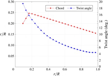
Chord-radius ratio and twist-angle distribution of the wind-turbine model blades (Lignarolo et al. Reference Lignarolo, Ragni, Krishnaswami, Chen, Simão Ferreira and Van Bussel2014).

2.3. Experimental set-up and test conditions
2.3.1. Wind-tunnel and wind-turbine model
Experiments have been conducted in the Open-Jet Facility at the Aerospace Engineering Department of TU Delft. The wind tunnel has an octagonal test section with an equivalent diameter of 3 m and a contraction ratio of 3:1, delivering a uniform stream with approximately 0.5 % turbulent intensity at 1 m from the jet exit and lower than 2 % at 6 m from it. The uniform-flow region also reduces at 6 m from the jet exit from
 $3\times 3~\text{m}^{2}$
to
 $2\times 2~\text{m}^{2}$
. A detailed characterisation of the wind-tunnel flow can be found in Lignarolo et al. (Reference Lignarolo, Ragni, Krishnaswami, Chen, Simão Ferreira and Van Bussel2014). The wind tunnel is driven by a fan with an electrical engine of 500 kW and the temperature is kept constant by a heat exchanger which provides up to 350 kW of cooling power. A two-bladed horizontal-axis wind turbine with a diameter
 $D=0.6~\text{m}$
has been designed for an optimal tip-speed ratio
 ${\it\lambda}={\it\upsilon}R/U_{\infty }=6$
, where
 $R$
is the rotor radius and
 ${\it\upsilon}$
the rotational speed. The rotor blade is developed from an Eppler E387 airfoil with 9.06 % thickness (Selig et al.
Reference Selig, Guglielmo, Broeren and Giguère1995) with a twist distribution from 4.4° at the tip to 19.4° at the root (see figure 1). The maximum blade chord is 0.074 m at
 $r/R=0.18$
(with
 $r$
being the radial coordinate).
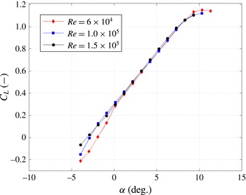
 $C_{L}{-}{\it\alpha}$
curves of airfoil E387 are presented in figure 2. The analysis is repeated for two different tip-speed ratios, namely
 ${\it\lambda}=6$
and
 ${\it\lambda}=4.8$
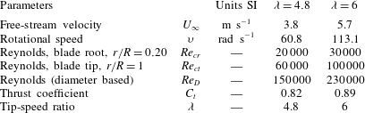
, respectively, with free-stream velocities of
 $U_{\infty }=5.7$
and
 $3.8~\text{m s}^{-1}$
and rotational speeds of
 ${\it\upsilon}=113.1$
and
 $60.8~\text{rad s}^{-1}$
. The former value is the design tip-speed ratio and represents the optimum working condition of the machine. For both tip-speed ratios, wind speed and rotational speed are chosen in order to fulfil several requirements, such as avoiding tower vibration due to possible resonances with the vortex shedding and the blade rotation and achieving a high Reynolds number. As shown in Widnall (Reference Widnall1972) and Felli et al. (Reference Felli, Camussi and Di Felice2011), the tip-speed ratio will modify the pitch of the tip-vortex helical filament, having a strong impact on the leapfrogging location, the latter being inversely proportional to
 ${\it\lambda}$
. There were three main drivers for the blade design: the first was constant circulation along the blade span at the design tip-speed ratio in order to have most of the vorticity trailing only at the tip and at the root, with no trailing vorticity at other blade locations. The second was to achieve attached-flow conditions over the entire span, which led to low angles of attack and low lift coefficients, and therefore to a large average chord. The third requirement was to achieve a relatively large Reynolds number, in turn leading to a large chord and high rotational speed. At the experimental conditions, the maximum chord-based Reynolds number achieved is
 $\mathit{Re}_{c}=100\,000$
at the blade tip, as indicated in table 1 (Lignarolo et al.
Reference Lignarolo, Ragni, Krishnaswami, Chen, Simão Ferreira and Van Bussel2014). In calculating the latter, the relative velocity of the wind on the blades has been used as reference. The blades have been manufactured in aluminium by CNC machinery. The blades are installed on the nacelle hub with a pitch-angle difference of 0.5°, which acts as a systematic trigger for the wake instability, similarly to the studies of Bolnot et al. (Reference Bolnot, Le Dizès and Leweke2014) and Odemark & Fransson (Reference Odemark and Fransson2013). The values of the thrust coefficients
 $C_{t}$
for the two experimental conditions shown in table 1 have been calculated with an external six-component balance. The device is provided with six Wheatstone bridges, which are able to measure three components of force, in the axial, spanwise and vertical directions, and three components of moments, for roll, pitch and yaw. For the present thrust measurements, only the axial force component is relevant and has been reported in Lignarolo et al. (Reference Lignarolo, Ragni, Krishnaswami, Chen, Simão Ferreira and Van Bussel2014). The nacelle is designed to reduce to minimum its impact on the flow while housing a DC brushless motor, a gearbox, a Hall encoder and an optical trigger (opto-coupler TCST 2103) which provides a one pulse per revolution signal allowing the PIV synchronisation; the nacelle has a diameter of 0.038 m (6.3 % of the rotor diameter). The DC brushless motor has a nominal voltage of 12 V and a maximum power of 125 W. It is a four-quadrant motor, able to act as a drive or a brake, depending on the loading. In operation, the motor provides a torque to the hub which is equal and opposite to the that exerted by the wind on the blades, thus maintaining a constant rotational speed. The extra energy is then dissipated by a large resistor at the base of the tower. Given the present measurement domain and available equipment, the Reynolds number achievable based on the turbine diameter and free-stream wind speed ranges from
 $\mathit{Re}=1.5\times 10^{5}$
to
 $2.3\times 10^{5}$
for
 ${\it\lambda}=4.8$
and
 ${\it\lambda}=6$
respectively. These values are an order of magnitude lower than in full-scale operating conditions. However, previous studies have demonstrated that the wake exhibits a low dependency on the Reynolds number (Whale et al.
Reference Whale, Anderson, Bareiss and Wagner2000). Chamorro, Arndt & Sotiropoulos (Reference Chamorro, Arndt and Sotiropoulos2012) showed that the main flow statistics become independent of Reynolds number above the critical value
 $\mathit{Re}=9.3\times 10^{4}$
, sufficiently lower than the Reynolds number in the present study.
 $C_{L}$
–
 ${\it\alpha}$
curves of airfoil E387 from
 $\mathit{Re}=0.6\times 10^{5}$
to
 $\mathit{Re}=1.5\times 10^{5}$
(Lignarolo et al.
Reference Lignarolo, Ragni, Krishnaswami, Chen, Simão Ferreira and Van Bussel2014).

Test conditions for the two investigated tip-speed ratios.

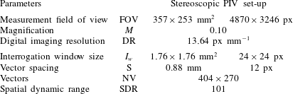
System parameters for the stereoscopic PIV measurements.

2.3.2. Stereoscopic particle image velocimetry
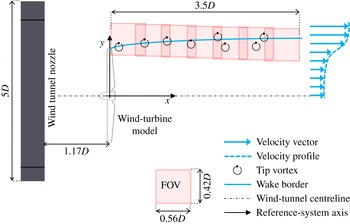
Stereoscopic PIV experiments are conducted, mapping the three-component velocity fields in the rotor wake; results are obtained via an average of the vector fields, as detailed in table 2. A stereoscopic PIV set-up has been installed on a traversing system able to scan the flow field in the wake of the horizontal-axis wind-turbine wake, as shown in figure 3. This measurement set-up has already proved suitable to obtain both the load distribution on the blade (Ragni, Oudheusden & Scarano Reference Ragni, Oudheusden and Scarano2011) and the evolution of vorticity in the wake of a wind turbine (Akay et al.
Reference Akay, Ferreira, Van Bussel and Herraez2012). The required illumination is provided by a Quantel Evergreen Nd:YAG laser system with an average output of
 $200~\text{mJ pulse}^{-1}$
. The laser light is shaped to form a 2 mm laser sheet of approximately 0.4 m width at the field of view. Two LaVision Imager Pro LX 16 Mpix (
 $4870\times 3246~\text{px}$
, 12 bits) cameras with a pixel pitch of
 $7.4~{\rm\mu}\text{m px}^{-1}$
are used to acquire images with a field of view of
 $0.357\times 0.253~\text{m}^{2}$
(
 $0.56D\times 0.42D$
), with an overlap between two adjacent FOVs of 0.05 m in the axial and radial directions (darker shade between the FOV in figure 3), obtained with two Nikon lenses of
 $f=180~\text{mm}$
and an aperture
 $f\#=2.8{-}4$
, at a magnification factor
 $M=0.10$
. The focusing plane has been slightly offset with respect to the laser plane (defocusing), to obtain an image of the particle of approximately 2–3 px. Therefore no bias error arising from the peak-locking effect has been observed (Westerweel Reference Westerweel1997). Seeding was provided in the test section by a SAFEX smoke generator with SAFEX MIX, able to produce liquid droplets of less than
 $1~{\rm\mu}\text{m}$
. The entire set-up was mounted on a traversing system able to translate over a two-dimensional area of approximately
 $1.2\times 0.9~\text{m}^{2}$
. An ensemble of 400 (phase-locked sampling), 720 (unconditioned sampling) double-frame recordings have been acquired and processed by LaVision Davis 8.1.4. In order to evaluate the digital range of the measurement system, estimation of the smallest and largest coherent structures within the wake flow can be performed. The smallest coherent structures in the flow, which are supposed to have a lifetime long enough to contribute to the statistics, are typically generated within the blade boundary layer and have a length scale of 20 times the wall units
 ${\it\lambda}^{+}$
(Stanislas, Perret & Foucaut Reference Stanislas, Perret and Foucaut2008; Ghaemi & Scarano Reference Ghaemi and Scarano2011). The latter is calculated as
 ${\it\lambda}^{+}={\it\nu}/u_{{\it\tau}}$
, where the friction velocity is estimated with a viscous simulation using the boundary-layer theory applied to the blade geometry (White Reference White1991). For this purpose, the TUDelft modification of the software XFoil has been used (van Rooij Reference van Rooij1996). At a tip-speed ratio of 6, the trailing-edge friction velocity at the tip location is
 $0.24~\text{m s}^{-1}$
and the wall unit is
 $62~{\rm\mu}\text{m}$
: this corresponds to a length scale for the smallest coherent structures of 1.24 mm. The large-scale motion in the rotor wake has the length scale of the blade chord, which has a maximum extent of 0.074 m. Therefore the ratio between the large-scale motion and the smallest coherent structures is
 $W_{str}=~60$
, which must be satisfied by the resolution of the measurement system (Herpin et al.
Reference Herpin, Wong, Stanislas and Soria2008). Interrogation windows of
 $24\times 24~\text{px}$
with 50 % overlap yields a resolution element of 1.76 mm and a vector spacing of 0.88 mm. In this configuration the final spatial dynamic range (SDR) in the streamwise direction is 101 (as detailed in table 2) and the smallest resolvable spatial variation is considered to be twice the size of the interrogation window. This does not allow one to capture the smallest scale at the tip location, but is considered sufficient for the downstream development, especially in the leapfrogging regime. By taking into consideration the combination of different fields of view (see figure 3), the SDR becomes 4.5 times larger.
Schematic top-view of the experimental layout (not to scale): wind tunnel exit, wind-turbine model and measurement domain obtained by the superposition of multiple and partly overlapping fields of view (FOV). Each squared window represents a FOV in the horizontal (
 $x{-}y$
) plane. The schematic also shows a qualitative impression of the wake border, of the unstable tip vortices and of the wake axial velocity profile.

3. Analysis of the tip-vortex instability
In § 3.1, the topology of the flow in the regime of leapfrogging vortices is shown, highlighting the vortex core locations, divergent and convergent separatrices and saddle points. The latter are of particular interest in the analysis of fluxes and turbulence production rate. Sections 3.2 and 3.3 comment on the distribution of the mean-flow kinetic-energy flux and turbulence production.
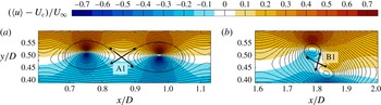
Normalised phase-locked average axial velocity field at
 ${\it\lambda}=4.8$
. Close-ups on the tip vortices before and during leapfrogging.

3.1. Vortex flow, cores and saddle points
The vortex cores can be identified after calculating the phase-locked vorticity field (see Lignarolo et al.
Reference Lignarolo, Ragni, Krishnaswami, Chen, Simão Ferreira and Van Bussel2014) as
 $\langle {\it\omega}_{z}\rangle =\partial \langle v\rangle /\partial x-\partial \langle u\rangle /\partial y$
, where the
 $z$
-direction corresponds to the out-of-plane direction in the rotor frame of reference (figure 3), and applying (3.1):
 $$\begin{eqnarray}x_{\mathit{core}}=\frac{\displaystyle \mathop{\sum }_{n,m}x_{n,m}\langle {\it\omega}_{z}\rangle _{n,m}\,\text{d}A}{\displaystyle \mathop{\sum }_{n,m}\langle {\it\omega}_{z}\rangle _{n,m}\,\text{d}A},\quad y_{\mathit{core}}=\frac{\displaystyle \mathop{\sum }_{n,m}y_{n,m}\langle {\it\omega}_{z}\rangle _{n,m}\,\text{d}A}{\displaystyle \mathop{\sum }_{n,m}\langle {\it\omega}_{z}\rangle _{n,m}\,\text{d}A},\end{eqnarray}$$
where
 $\text{d}A$
is the discrete portion of an area
 $A$
encompassing the vortex and
 $n$
and
 $m$
are column and row indices of the two-dimensional matrices
 $x,y$
and
 ${\it\omega}$
. The equation is the average of the position vector weighted over a distribution of vorticity (Ferreira Reference Ferreira2009). The convection velocity
 $U_{c}$
at the vortex cores can be calculated by estimating the time-average velocities
 $\bar{u}$
and
 $\bar{v}$
(see Lignarolo et al.
Reference Lignarolo, Ragni, Krishnaswami, Chen, Simão Ferreira and Van Bussel2014) at the locations of the vortex cores for several vortices at both tip-speed ratios. The axial convection velocity
 $U_{c}$
is estimated as
 $U_{c}/U_{\infty }=0.67\pm 0.002$
for
 ${\it\lambda}=4.8$
and
 $U_{c}/U_{\infty }=0.65\pm 0.005$
for
 ${\it\lambda}=6$
(with 95 % confidence interval), and can be considered constant in the region of interest. The vertical convection velocity is found to be almost two orders of magnitude smaller than
 $U_{c}$
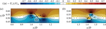
in the region swept by the vortex passage, and as such is neglected. The same assumption has been adopted by Antonia et al. (Reference Antonia, Chambers, Britz and Browne1986). Consequently, the velocity fields in figures 4 and 5 are representative of the two-dimensional velocity field
 $[\bar{u}+\tilde{u} -U_{c}]$
,
 $[\bar{v}+\tilde{v}]$
as seen by an observer travelling with the vortex convective velocity
 $U_{c}$
. The streamline pattern identifies the location of the saddle points between the vortex pairs and slopes of the convergent and divergent separatrices. The two close-ups of figures 4 and 5 show the pairwise organisation of the vortices, separated by streamline saddle points A1, B1, A2, B2. The two arrowed lines indicate the convergent and divergent separatrices connecting two consecutive vortices. The absolute inclination of the divergent separatrices with respect to the wake centreline varies during the wake evolution due to the wake expansion (which deflects the shear layer in the very near wake) and to the leapfrogging. The relative value of the separatrix inclination with respect to the vortex-pair middle plane was estimated to be approximately 40°, in good agreement with the findings of Antonia et al. (Reference Antonia, Browne, Bisset and Fulachier1987). This value is constant at all locations, also during the leapfrogging.
Normalised phase-locked average axial velocity field at
 ${\it\lambda}=6$
. Close-ups on the tip vortices before and during leapfrogging.

3.2. Mean-flow kinetic-energy flux
The rapid increase in the kinetic-energy content of the wake has been observed to begin after the tip vortices have paired and completed an approximately 90° rotation around their saddle points Lignarolo et al. (Reference Lignarolo, Ragni, Krishnaswami, Chen, Simão Ferreira and Van Bussel2014). This location coincides with the onset of a three-dimensional breakdown of the helical vortices, inducing a more efficient mixing, dominated by random fluctuations. Previous studies have shown that this phenomenon induces a reorientation of the azimuthal vorticity towards the streamwise direction, in turn enhancing the mixing (Widnall & Sullivan Reference Widnall and Sullivan1973; Yule Reference Yule1978; Violato & Scarano Reference Violato and Scarano2011). However, the relative importance of the coherent vortical structures and the random flow fluctuations in the transport of the mean-flow kinetic energy remains to be quantified in order to make a conclusive statement on the process dominating wake re-energising. For this purpose, it is useful to consider the spatial distribution of the mean-flow kinetic-energy flux. Prior to proceeding with the analysis, two spurious contributions affecting the phase-locked-average
 $u_{\mathit{RMS}}$
are quantified that arise from PIV measurement uncertainty. A typical value of 0.1 pixel standard-error is associated with a three-point fit of the correlation peak (see Ragni et al.
Reference Ragni, Ashok, Van Oudheusden and Scarano2009). For the 400 samples used in the phase averaging, the relative error on the turbulent velocity fluctuations
 $\langle u_{\mathit{RMS}}\rangle$
is estimated as 0.1 %, 0.3 % and 0.6 %, where
 $\langle u_{\mathit{RMS}}\rangle$
is 30 %, 10 % and 4 % of the free-stream velocity, respectively, which is a negligible contribution (see Benedict & Gould Reference Benedict and Gould1996; Humble Reference Humble2008). The second spurious effect is due to the so-called vortex wandering effect, namely the random fluctuation of the location of the vortex core in time (Dobrev et al.
Reference Dobrev, Maalouf, Troldborg and Massouh2008). An a posteriori evaluation of the importance of this aspect has been carried out by re-aligning all the images of each PIV dataset with the location of a chosen vortex core, respectively, in the near wake and in the leapfrogging region (see Vandernoot et al.
Reference Vandernoot, Barricau, Bézard and Boisson2008) at
 $x/D=~0.69$
and
 $x/D=1.45$
. The wandering of the vortex contributes to the
 $\langle u_{\mathit{RMS}}\rangle$
peaks at the vortex core locations, with an additional 3 % in the near wake and an additional 8 % in the leapfrogging region, but no effect of re-centring has been observed outside the vortex core, in the region where most of the analysis is carried out.
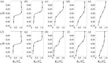
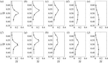
Radial profiles of mean-flow kinetic energy at five different locations in the wake shear layer at
 ${\it\lambda}=4.8$
(a–e) and
 ${\it\lambda}=6$
(f–j): (a,f)
 $x/D=0.2$
; (b,g) 0.7; (c,h) 1.4; (d,i) 2.4; (e,j) 3.4.

Figure 6 depicts the radial profiles of mean-flow kinetic energy at five different locations in the wake shear layer, whose transport in space for one phase is described by (2.7). The location at
 $x/D=1.4$
is within the leapfrogging region and shows the characteristic splitting of the shear layer, also noted in Lignarolo et al. (Reference Lignarolo, Ragni, Krishnaswami, Chen, Simão Ferreira and Van Bussel2014). The terms
 $\langle \tilde{{\it\Phi}}\rangle =-\bar{u}\langle \tilde{u} \tilde{v}\rangle$
and
 $\langle {\it\Phi}_{s}\rangle =-\bar{u}\langle u_{s}v_{s}\rangle$
in (2.8) represent the fluxes in the
 $x{-}y$
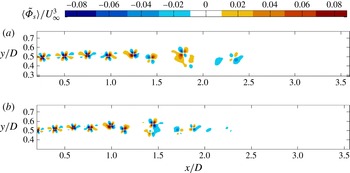
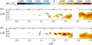
plane of the mean-flow kinetic energy at a selected phase by the respective actions of the periodic (figure 7) and random fluctuations (figure 8). Positive values represent mean downward fluxes of kinetic energy and, therefore, energy entrained in the inner part of the wake. By looking at both tip-speed ratios, two zones can be identified in figures 7 and 8. The first zone is located before the vortex leapfrogging where the wake expansion occurs. In this region the tip vortices are the only ones determining a mean-flow kinetic energy transport across the wake layer – both positive and negative contributions of similar magnitude are present in this area. The second zone is located after the wake instability and the tip-vortex breakdown. This area is characterised by solely positive flux, corresponding to a downward net entrainment of kinetic energy. Here the random turbulent motion has a dominant role in the recovery process entraining flow towards the inner region of the wake. The beginning of the second zone can be identified in proximity to the position where the vortex pairs are about to complete a 90° rotation around their saddle points. This is located at
 $x/D\sim 1.5$
for
 ${\it\lambda}=6$
and at
 $x/D\sim 1.7$
for
 ${\it\lambda}=4.8$
. It must be noted that at both tip-speed ratios the phenomenon happens after the same number of revolutions of the tip-vortex helix.
Mean-flow kinetic-energy transport due to the periodic fluctuation at
 ${\it\lambda}=4.8$
(a) and
 ${\it\lambda}=6$
(b).

Mean-flow kinetic-energy transport due to the random fluctuations, at
 ${\it\lambda}=4.8$
(a) and
 ${\it\lambda}=6$
(b).

In order to evaluate the net transport of kinetic energy,
 $\langle \tilde{{\it\Phi}}\rangle$
and
 $\langle {\it\Phi}_{s}\rangle$
are integrated and averaged in space. Figures 9 and 10 (respectively for
 ${\it\lambda}=4.8$
and
 ${\it\lambda}=6$
) show two different spatial integrals of the mean-flow kinetic-energy flux. The quantities
 $IF_{per}$
and
 $IF_{rdm}$
are the area average of
 $\langle \tilde{{\it\Phi}}\rangle$
and
 $\langle {\it\Phi}_{s}\rangle$
, respectively, calculated in different sections of the wake shear layer as in (3.2):
 $$\begin{eqnarray}IF_{per}=\frac{1}{AU_{\infty }^{3}}\int _{A}\langle \tilde{{\it\Phi}}\rangle \,\text{d}x\,\text{d}y,\quad IF_{rdm}=\frac{1}{AU_{\infty }^{3}}\int _{A}\langle {\it\Phi}_{s}\rangle \,\text{d}x\,\text{d}y,\end{eqnarray}$$
where
 $A$
is the area of each section. The streamwise extension of a section corresponds to the distance travelled by a vortex during a complete blade rotation. The limits of each section are indicated by the black arrows in figure 8 and reported in the
 $x$
-axes of figures 9 and 10(a). The quantities
 $\mathit{CSF}_{per}$
and
 $\mathit{CSF}_{rdm}$
are the cumulative sums of the area integral of
 $\langle \tilde{{\it\Phi}}\rangle$
and
 $\langle {\it\Phi}_{s}\rangle$
respectively, calculated as in (3.3):
 $$\begin{eqnarray}\mathit{CSF}_{per}=\frac{1}{\text{d}AU_{\infty }^{3}}\int _{0}^{x}\int _{in}^{out}\langle \tilde{{\it\Phi}}\rangle \,\text{d}x\,\text{d}y,\quad \mathit{CSF}_{rdm}=\frac{1}{\text{d}AU_{\infty }^{3}}\int _{0}^{x}\int _{in}^{out}\langle {\it\Phi}_{s}\rangle \,\text{d}x\,\text{d}y.\end{eqnarray}$$
The infinitesimal area integrals
 $\int _{in}^{out}\langle \tilde{{\it\Phi}}\rangle \,\text{d}x\,\text{d}y/\text{d}A$
and
 $\int _{in}^{out}\langle {\it\Phi}_{s}\rangle \,\text{d}x\,\text{d}y$
are calculated across the wake shear layer, from innermost to the outermost radial locations available in the section
 $\text{d}A$
with streamwise extension
 $\text{d}x$
. This quantity allows one to observe the streamwise evolution of the total energy entrained in the wake.
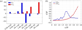
Spatial integrals
 $IF_{per}$
and
 $IF_{rdm}$
in different sections of the wake shear layer (a) and the cumulative sums
 $\mathit{CSF}_{per}$
and
 $\mathit{CSF}_{rdm}$
of the periodic and random flux respectively (b) at
 ${\it\lambda}=4.8$
.

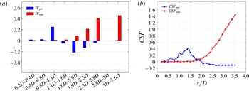
Spatial integrals
 $IF_{per}$
and
 $IF_{rdm}$
in different sections of the wake shear layer (a) and the cumulative sums
 $\mathit{CSF}_{per}$
and
 $\mathit{CSF}_{rdm}$
of the periodic and random flux respectively (b) at
 ${\it\lambda}=6$
.

At
 ${\it\lambda}=6$
the values of
 $IF_{per}$
in figure 10(a) are generally close to zero, also in the proximity of the rotor, where the periodic fluctuations are stronger. This shows that in fact the positive and negative flux areas depicted in figure 7 are compensating for each other. A peak of positive flux in the area between
 $0.8D$
and
 $1.1D$
is visible immediately before the beginning of the leapfrogging region. Past this location the value of the flux is generally negative, and quickly returns to zero after
 $2.4D$
.
The
 $\mathit{CSF}_{per}$
curve in figure 10(b) shows that there is a net positive kinetic-energy transport until
 $1.5D$
(the location where the tip vortices have paired and completed a 90° rotation around their saddle points), which then turns into a decreasing trend due to the beginning of an overall negative transport. The total balance of the transported energy by the action of the periodic motion is nearly zero, as indicated by the value of
 $\mathit{CSF}_{per}$
after
 $2D$
.
Quadrant analysis applied to
 $\langle {\it\Phi}_{s}\rangle$
at
 ${\it\lambda}=6$
. (a–d) Sum of the sweep and ejection events causing a positive flux. (e–h) Sum of inward and outward interactions, causing a negative flux. In the first three locations, the vortex pair is followed during the leapfrogging process. The last location is taken in the far wake.

The values of
 $IF_{rdm}$
in figure 10(a) are positive everywhere, characterised by a very low magnitude in the near wake and a sudden rapid increase in the region between
 $1.1D$
and
 $1.7D$
, as also evident in the cumulative sum in figure 10(b).
In figure 9(a), the values of
 $IF_{per}$
at
 ${\it\lambda}=4.8$
have a behaviour similar to that exhibited at
 ${\it\lambda}=6$
, with values everywhere very close to zero, with the exception of the leapfrogging region, where the positive flux is much higher and followed by a negative peak of comparable intensity. This inversion of the direction of
 $\langle \tilde{{\it\Phi}}\rangle$
present in both tip-speed ratios is strictly related to the orientation of the vortex pairs, and will be discussed in § 4.
The cumulative sum
 $\mathit{CSF}_{per}$
in figure 9(b) again shows a peak at the location where the tip vortices are about to complete a 90° rotation and the
 $\langle \tilde{{\it\Phi}}\rangle$
inversion takes place, but in this case it does not fall to zero, meaning that for this tip-speed ratio the total kinetic energy transported by periodic motion is still positive (although very low) in the wake region considered.
 $\mathit{CSF}_{per}$
and
 $IF_{per}$
at
 ${\it\lambda}=4.8$
have a general behaviour similar to that at
 ${\it\lambda}=6$
.
The analysis of the mean-flow kinetic-energy flux has shown the absence of considerable mixing and entrainment of kinetic energy in the very near wake under the actions of both periodic and random flow fluctuations. Also, the analysis of the total balance (
 $\mathit{CSF}_{per}$
curves) has shown how the tip vortices have a zero or negligible contribution to the mixing, confirming the hypothesis of Medici (Reference Medici2005) about the tip-vortex shielding effect.
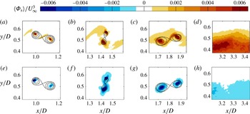
Figure 11 shows the results of quadrant analysis of the mean-flow kinetic-energy flux due to the random fluctuations (four close-ups in selected shear-layer sections). Only the results for
 ${\it\lambda}=6$
have been shown, since
 ${\it\lambda}=4.8$
leads to the same conclusions. Positive fluxes due to sweep and ejection events have been summed together (figure 11
a–d), as the negative contributions due to outward and inward interactions (figure 11
e–h). In the near-wake region, the location of the tip vortices has been visualised with streamlines forming convergent and divergent separatrices. The contours in the first and second regions show that most of the random fluctuations in the wake shear layer are due to sweep and ejection events, causing a positive flux of mean-flow kinetic energy. These positive contributions are located in the regions along divergent separatrices. Some peaks of the flux are also observed at the very centre of the vortex cores. The latter, however, are ascribed to a locally higher experimental error, as discussed in § 3.2. This means that in the random fluctuations along the divergent separatrices the terms
 $u_{s}$
and
 $v_{s}$
are anticorrelated. In the second region, the divergent separatrices shows a peak of inward and outward interactions causing a negative flux: the process of leapfrogging induces a reorientation of the turbulent fluctuations, leading the
 $u_{s}{-}v_{s}$
correlation to locally switch sign. The concept is further developed in § 3. In the far wake (fourth location), after the tip-vortex breakdown, sweep and ejection events induce a positive flux encompassing the whole shear layer. Negative contributions, caused by outward and inward interactions, are much less frequent and concentrated in the proximity of the vortex cores only.
Figure 12 shows the cumulative sum
 $\mathit{CSF}_{per}$
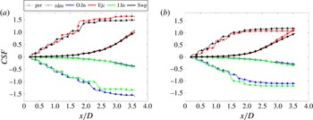
(dashed lines with triangles) of the spatially-integrated contribution of the periodic motion to the total mean-flow kinetic-energy flux decomposed into four quadrant contributions (both tip-speed ratios). As expected, positive contributions (sweep and ejection events) and negative contributions (outward and inward interactions) are of the same magnitude, leading to a quasizero net flux, with the exception of the region preceding the leapfrogging. Figure 12 (bold lines with circles) shows the results of the quadrant analysis applied to the cumulative sum
 $\mathit{CSF}_{rdm}$
of the spatially integrated flux. The total of the sweep and ejection events contribute equally to the total positive flux, as do the inward and outward interactions to the total negative flux, with the former having a magnitude about four times larger than the latter. It must be noted that the sum of the four quadrant contributions (in both random and periodic motions) results in the same curves plotted in figures 9 and 10.
Quadrant analysis applied to
 $\langle {\it\Phi}_{s}\rangle$
at
 ${\it\lambda}=4.8$
(a) and at
 ${\it\lambda}=6$
(b). The images show the cumulative sum
 $\mathit{CSF}_{per}$
and
 $\mathit{CSF}_{rdm}$
decomposed into four quadrant contributions. The dashed lines with triangles and the bold lines with circles represent the contributions of the periodic and random motions respectively. The abbreviations O.in, Ejc, I.In and Swp refer to outward interactions, ejections, inward interactions and sweeps respectively.

3.3. Production of turbulent kinetic energy
Figure 13 depicts the radial profiles of the turbulence intensity at five different locations in the wake shear layer. This represents the turbulence relative to the unconditioned-averaged field, as such including contributions from both periodic and random fluctuations with no distinction. The production of turbulence for one phase is described by (2.10).
Radial profiles of turbulence intensity relative to the unconditioned-averaged field at five different locations in the wake shear layer at
 ${\it\lambda}=4.8$
(a–e) and
 ${\it\lambda}=6$
(f–j). Data from Lignarolo et al. (Reference Lignarolo, Ragni, Krishnaswami, Chen, Simão Ferreira and Van Bussel2014): (a,f)
 $x/D=0.2$
; (b,g) 0.7; (c,h) 1.4; (d,i) 2.4; (e,j) 3.4.

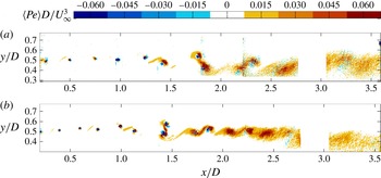
Figure 14 shows the contour level of the normalised phase-locked production of turbulent kinetic energy
 $\langle Pe\rangle$
calculated as in (2.10). This quantity represents the decay into turbulence of the kinetic energy of the mean flow and of the periodic flow structures. In figure 14, the contours of
 $\langle Pe\rangle$
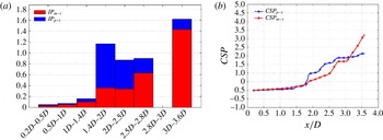
are stronger in the region along the divergent separatrices, as well as in the proximity of the vortex core. The production of turbulence values along the divergent separatrix for both tip-speed ratios reach their maxima in the leapfrogging region. This finding shows similarities both to the behaviour of the vortical structures in the cylindrical shear layer of a wind-turbine wake and in bluff-body wakes or planar mixing layers. These findings confirm the previous observations of Hussain (Reference Hussain1981), who noted that the turbulence is produced mainly in the braids between the large vortices along the divergent separatrix and then transported to and accumulated in the vortices, as well as those of Cantwell & Coles (Reference Cantwell and Coles1983) and Antonia et al. (Reference Antonia, Browne, Bisset and Fulachier1987), who showed that the saddle points between two consecutive vortices are zones of large production of turbulent kinetic energy.
Total turbulent kinetic-energy production
 $\langle Pe\rangle =\langle Pe_{p-t}\rangle +\langle Pe_{m-t}\rangle$
at
 ${\it\lambda}=4.8$
(a) and
 ${\it\lambda}=6$
(b).

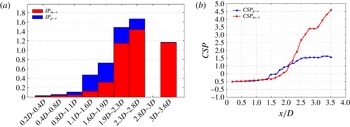
Figures 15 and 16 (respectively for
 ${\it\lambda}=4.8$
and
 ${\it\lambda}=6$
) show the spatial integrals of the turbulence production, similarly to that presented in § 3.2. The quantities
 $IP_{m-t}$
and
 $IP_{p-t}$
are the area average of
 $\langle Pe_{m-t}\rangle$
and
 $\langle Pe_{p-t}\rangle$
, respectively, calculated in different sections of the wake shear layer as in (2.8):
 $$\begin{eqnarray}IP_{m-t}=\frac{D}{AU_{\infty }^{3}}\int _{A}\langle Pe_{m-t}\rangle \,\text{d}x\,\text{d}y,\quad IP_{p-t}=\frac{D}{AU_{\infty }^{3}}\int _{A}\langle Pe_{p-t}\rangle \,\text{d}x\,\text{d}y,\end{eqnarray}$$
where
 $\langle Pe_{m-t}\rangle$
is the phase-locked turbulence production due to the decay of the mean-flow kinetic energy and
 $\langle Pe_{p-t}\rangle$
the phase-locked turbulence production due to the decay of the organised periodic structures. The sections (indicated by
 $A$
) are the same as in (3.2). The quantities
 $\mathit{CSF}_{m-t}$
and
 $\mathit{CSF}_{p-t}$
are the cumulative sums of the area integral of
 $\langle Pe_{m-t}\rangle$
and
 $\langle Pe_{p-t}\rangle$
, respectively, calculated as in (3.5):
 $$\begin{eqnarray}\mathit{CSF}_{m-t}=\frac{D}{\text{d}AU_{\infty }^{3}}\int _{0}^{x}\int _{in}^{out}\langle Pe_{m-t}\rangle \,\text{d}x\,\text{d}y,\quad \mathit{CSF}_{p-t}=\frac{D}{\text{d}AU_{\infty }^{3}}\int _{0}^{x}\int _{in}^{out}\langle Pe_{p-t}\rangle \,\text{d}x\,\text{d}y.\end{eqnarray}$$
As in (3.3), the infinitesimal area integrals are calculated across the wake shear layer, from innermost to the outermost radial locations available in the section
 $\text{d}A$
with streamwise extension
 $\text{d}x$
. Although minor regions characterised by a negative production were visible in figure 14, the balance is positive in total and in each wake section: this is valid for both contributions
 $\langle Pe_{m-t}\rangle$
and
 $\langle Pe_{p-t}\rangle$
.
Spatial integrals of the production
 $IP_{m-t}$
and
 $IP_{p-t}$
for different sections of the wake shear layer (a) and the cumulative sum of the production
 $\mathit{CSP}_{p-t}$
and
 $\mathit{CSP}_{m-t}$
(b) at
 ${\it\lambda}=4.8$
.

Spatial integrals of the production
 $IP_{m-t}$
and
 $IP_{p-t}$
for different sections of the wake shear layer (a) and the cumulative sum of the production
 $\mathit{CSP}_{p-t}$
and
 $\mathit{CSP}_{m-t}$
(b) at
 ${\it\lambda}=6$
.

At both tip-speed ratios, it is evident that the very near wake is characterised by a negligible rate of production. The production due to the decay of the periodic structures is maximum in the instability region where the tip vortices break down, after which it decreases to negligible values. This is evident in the steep increase of the
 $\mathit{CSP}_{p-t}$
in figure 15(b) at
 ${\it\lambda}=4.8$
between
 $1.5D$
and
 $2D$
and by the more gradual increase in figure 16(b) at
 ${\it\lambda}=6$
between
 $1.5D$
and
 $2.5D$
. Past these locations, the
 $\mathit{CSP}_{p-t}$
curves tend to flatten, indicating no further turbulence production from the decay of the periodic structures, because tip vortices have completed their breakdown process. The production due to the mean-flow kinetic-energy decay
 $\langle Pe_{m-t}\rangle$
also starts increasing in the instability region, together with
 $\langle Pe_{p-t}\rangle$
, for both values of
 ${\it\lambda}$
, from a quasizero value in the near wake, but after the vortex breakdown it maintains large values.
4. Effect of orientation of the flow fluctuations
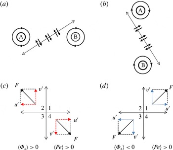
The analysis of figures 9(a) and 10(a) indicated an inversion of the flux
 $\langle \tilde{{\it\Phi}}\rangle$
direction, present in both tip-speed ratios, although at a different magnitude (at
 ${\it\lambda}=4.8$
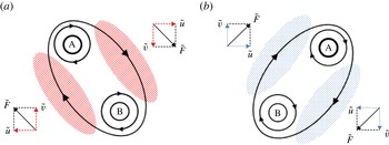
the passage from positive to negative flux is more pronounced). This inversion is caused by the different orientation of the tip-vortex pairs during the leapfrogging process. In particular, in the initial stage of leapfrogging, the vortex pairs have a negative inclination (see between
 $1.4D$
and
 $2D$
at
 ${\it\lambda}=4.8$
and between
 $0.8D$
and
 $1.1D$
at
 ${\it\lambda}=6$
in figure 14), which leads to a strong anticorrelation of
 $\tilde{u}$
and
 $\tilde{v}$
and to positive peaks of
 $\langle \tilde{{\it\Phi}}\rangle$
. In the later stage of leapfrogging, the vortex pairs show a positive inclination (see between
 $2D$
and
 $2.5D$
at
 ${\it\lambda}=4.8$
and between
 $1.6D$
and
 $1.9D$
at
 ${\it\lambda}=6$
in figure 14), with
 $\tilde{u}$
and
 $\tilde{v}$
being oriented so as to produce a negative peak of
 $\langle \tilde{{\it\Phi}}\rangle$
. This behaviour is depicted schematically in figure 17. The results suggest that the magnitude of the inversion (which is different for the two tip-speed ratios) depends on the angle of the vortex pair with respect to the wake centreline, namely on the phase of the pairing process. As a matter of fact, despite measurements being taken at the same phase of rotation of the turbine, vortex pairing and leapfrogging happen at different locations at different tip-speed ratios. In the selected phase, the vortex pairs at
 ${\it\lambda}=6$
have a smaller inclination compared to
 ${\it\lambda}=4.8$
, which causes the smaller magnitude of the inversion visible in figure 9(a).
Change of orientation of the vortex pairs. On the left, the initial stage of leapfrogging (vortex A leaps over vortex B) causes a negative inclination of the vortex pair. The marked areas indicate where the highest flux is (red stripes and blue dots indicate positive and negative flux respectively). The bold lines depicts schematically the streamlines and the black arrows indicate the direction of the flow fluctuation
 $\tilde{F}$
. The smaller arrows indicate the direction of the components
 $\tilde{u}$
and
 $\tilde{v}$
(dashed red arrows indicate anticorrelation and dotted blue arrows indicate correlation).

In figure 7, the flux
 $\langle \tilde{{\it\Phi}}\rangle$
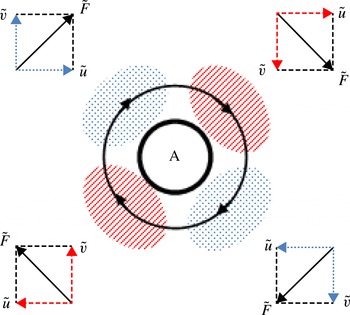
exhibits a peculiar four-lobed structure, which is known from previous literature, such as in the study of Hussain (Reference Hussain1983). Figure 18 schematises this behaviour, showing the different orientations of
 $\tilde{u}$
and
 $\tilde{v}$
around each vortex and the origin of the alternating negative and positive flux regions.
Schematic representation of the mean-flow kinetic-energy transport induced by a single vortex. The marked areas indicate the regions where the highest flux occurs (red stripes and blue dots indicate positive and negative flux respectively). The black arrows indicate the direction of the induced velocity fluctuation
 $\tilde{F}$
. The smaller arrows indicate the direction of the components
 $\tilde{u}$
and
 $\tilde{v}$
(dashed red arrows indicate anticorrelation and dotted blue arrows indicate positive correlation).

As far as random motion is concerned, the quadrant analysis in figure 11 indicates a local change of flux orientation, which, from a positive value in the braid region along the divergent separatrix, switches to negative values during the pairing and leapfrogging phase, and eventually reacquires positive values. This is explained in figure 19, which shows the different orientations of the random fluctuations
 $u_{s}$
and
 $v_{s}$
in the braid regions between two pairing vortices. Considering the orientation of the separatrices and the results of the quadrant analysis, it can be deduced that random fluctuations are always at an opposite inclination with respect to the divergent separatrices, keeping this relative orientation during the leapfrogging process. In particular, it was calculated that the angle between the random fluctuations and the divergent separatrices is roughly
 $80^{\circ }\pm 15^{\circ }$
at any location. The contour in figure 14(b) shows that, despite the changing absolute orientation of the
 $u_{s}$
and
 $v_{s}$
, the turbulence production stays positive, showing that while the mean-flow kinetic-energy flux depends on the inclination of the vortex pairs, the turbulence production depends only on the modulus of the random fluctuations. This behaviour is synthesised at figure 19(c,d).
Change of orientation of the random fluctuations
 $u_{s}$
and
 $v_{s}$
during leapfrogging. (a,c) Before leapfrogging,
 $u_{s}$
and
 $v_{s}$
have opposite inclinations with respect to the divergent separatrix and are anticorrelated, leading to a positive flux
 $\langle {\it\Phi}_{s}\rangle$
and positive turbulence production
 $\langle Pe\rangle$
. (b,d) During the leapfrogging
 $u_{s}$
and
 $v_{s}$
keep their orientation relative to the divergent separatrix, but show positive correlation, leading to a negative flux
 $\langle {\it\Phi}_{s}\rangle$
and positive turbulence production
 $\langle Pe\rangle$
(see figure 18 for arrow definitions).

5. Conclusions
An experimental investigation has been performed using SPIV to study the evolution of the vortex structure in the wake of a 0.6 m diameter horizontal-axis wind turbine and the influence of the pairing instability of the tip-vortex filaments (so-called leapfrogging) on the evolution of the far-wake turbulence production and mean-flow kinetic-energy transport, which in turn affects the wake re-energising process. The analysis of the interacting vortex pairs shows a general structure in agreement with previous studies on bluff-body wakes and planar jets. In a previous publication (Lignarolo et al.
Reference Lignarolo, Ragni, Krishnaswami, Chen, Simão Ferreira and Van Bussel2014), our qualitative analysis of the flow statistics revealed a major difference between the unconditioned-average and the phase-locked average turbulence-intensity. In the present investigation, transport of the mean-flow kinetic energy and the production of turbulence have been quantified to distinguish the role of periodic structures and random flow fluctuations in turbulence mixing and in turn to the wake re-energising process. The study demonstrates the fundamentally different roles of the vortex structures and turbulent fluctuations in the dynamics of wake turbulence. Both kinds of flow structures are normally accounted for in the estimation of what, in wind-energy jargon, is called ‘added turbulence’. The latter represents the flow turbulence caused by the presence of the turbine, which is added to the ambient turbulence (Crespo, Hernández & Frandsen Reference Crespo, Hernández and Frandsen1999). This includes both periodic and random velocity fluctuations, which are not separated in a classical double Reynolds decomposition. This leads to the well-known peaks of turbulence intensity close to the rotor at the blade-tip location. However, this is not theoretically correct. In fact, as pointed out by Yule (Reference Yule1978), a vortex is ‘the flow field accompanying a concentrated, continuous, coherent distribution of vorticity which is uniform in the direction of the vorticity vector and which grows in scale by viscous diffusion alone’, whereas ‘an eddy may be described as a vorticity-containing region of fluid which can be identified as moving as a coherent structure in a flow’. Also, as demonstrated in this analysis, the concentrated tip vortices in the near wake provide a strong contribution to the added turbulence, but do not take part in the mixing and the mean-flow kinetic-energy entrainment. Fluctuations due to the passage of tip vortices cannot as such be treated as turbulence, although they obey the same laws of vorticity transport, as they are determined by the Navier–Stokes equations. The distinction between the two flow structures is not sharp, but it is their predictable feature (namely periodicity, in this case) that can be used as distinction. The analysis of the mean-flow kinetic-energy flux suggests the presence of two zones characterised by a different mixing. In the first zone the tip vortices inhibit mixing of the wake during its expansion; in the second zone the leapfrogging causes a sudden increase of the net entrainment of the mean-flow kinetic energy and generates a more efficient mixing by the action of random flow motion, contributing to the wake re-energising process. The result is in accordance with the hypothesis of Medici (Reference Medici2005), who stated that the near-wake tip vortices are acting as a shield, preventing the wake from mixing with the outer flow. Quadrant analysis of the random flow fluctuations showed that the total of sweep and ejection events contribute equally to the total positive flux. Also inward and outward interactions have equal contributions to the total negative flux. The process of leapfrogging causes a reorientation of the turbulent fluctuations, leading to the
 $u_{s}{-}v_{s}$
correlation switching sign locally along the divergent separatrix. Following tip-vortex breakdown, sweep and ejection events occupy the whole shear-layer thickness, having total values about four times larger than the inward and outward interactions, concentrated in the proximity of the vortex cores only. The analysis of the production of turbulence shows very low values in first region, with an abrupt increase of production rate in the leapfrogging zone. This confirms that the vortex system of the near wake plays an important role in the production of turbulence and that eddy-viscosity models (only based on mean velocity gradients) fail to represent turbulence production in the near wake of a wind turbine. The present analysis has been conducted for a two-blade horizontal-axis wind turbine, but the method used and the main conclusions will keep their validity in the more common three-blade case. The expected changes will be a more unstable wake, with earlier leapfrogging, as shown experimentally by Felli et al. (Reference Felli, Camussi and Di Felice2011); also, the unstable tip vortices will not form pairs, but groups of three, as shown in the visualisation of Bolnot et al. (Reference Bolnot, Le Dizès and Leweke2014). The study has been performed at low turbulence intensity, to separate the problem of the flow mixing caused by the external turbulence from that caused by the turbulence induced directly by the wind turbine, and give full control over the tip-vortex instability. Our next step in this research will be to perform similar experiments with an increased inflow turbulence and analyse the sensitivity of the wake system to the free-stream flow fluctuations. In the presence of higher ambient turbulence, as shown in Ivanell (Reference Ivanell2009), the external flow fluctuations would introduce additional perturbations, which would trigger an earlier tip-vortex spiral instability, causing the leapfrogging to move upstream. The present research explains the dominant effect that the wake instability has on wake mixing, already expressed in a qualitative way by previous literature. This suggests a convenient way to further investigate how to design and operate wind turbines in wind farms in order to generate unstable wakes and to have a control on the wake recovery process, by considering the stability and re-energising properties of the wake as one of the design parameters that could be used in future wind-turbine rotors.