I. INTRODUCTION
Thermal transport properties of individual carbon-based nanomaterials, such as carbon nanotubes (CNTs) and graphene, have been reported to be largely uni- or bidirectional, respectively. For example, single-walled carbon nanotubes (SWCNTs) have been shown to possess extraordinarily high thermal conductivity along their longitudinal direction,Reference Berber, Kwon and Tomanek1–Reference Che, Cagin and Goddard4 while the single atomic layer graphene (SLG) is documented to have a thermal conductivity higher than SWCNTs along the graphene layer (in-plane) directionReference Balandin, Ghosh, Bao, Calizo, Teweldebrhan, Miao and Lau5–Reference Cai, Moore, Zhu, Li, Chen, Shi and Ruoff7 but relatively low out-of-plane thermal conductivity.Reference Sun, Stroscio and Dutta8 Three-dimensional (3D) pillared SWCNT–graphene nanostructures, comprising of unit cells with graphene layers as floors and SWCNTs as pillars, are being considered as the next-generation thermal interface materials. These hybrid nanomaterials capitalize on the excellent unidirectional thermal properties of SWCNTs and the in-plane thermal properties of SLGs, to develop lightweight structures with attractive in-plane and out-of-plane thermal transport characteristics. Additionally, CNTs and graphene are compositionally similar: both nanomaterials are made up of the same element carbon and they essentially consist of the same orbital hybridization (sp 2, other than at the edges). Although the carbon atoms at the CNT–graphene interface may not be sp 2 bonded (due to the numerous possibilities of attachment between the nanotube and graphene sheet), nonetheless, the similar constitution of the two materials reduces mismatch of the lattice vibrational spectra at the SWCNT-graphene junction. Theoretically, this implies that the impact of the junction encumbrance is kept to a minimum. Phonons propagating from the nanotube into the graphene sheet (or from graphene sheet to nanotube) are expected to encounter reduced phonon scattering at the interface and, therefore, a smaller thermal boundary (Kapitza) resistance.
Varshney et al.Reference Varshney, Patnaik, Roy, Froudakis and Farmer9 were the first to examine thermal transport properties of 3D pillared graphene nanostructures (PGNs) and showed that such 3D nanostructures ensure good in-plane as well as out-of-plane thermal conductivities. Loh et al.Reference Loh, Teo and Tay10 showed that the long wave length out-of-plane modes contribute significantly to thermal transport in such 3D PGNs. In addition, Loh et al.Reference Loh, Teo and Tay11 used molecular dynamics (MD) studies to investigate the effects of mechanical strain on the interfacial phonon dynamics in the PGNs. From their work, they concluded that there was a strong relationship between the strained PGN pillar lattice structure, interfacial phononics, and thermal boundary resistance.
More recently, rapid progress in synthesis and processing of materials on the nanometer length scale has provided exciting new possibilities for realizing such 3D nanomaterials in the laboratory. For example, Fan et al.Reference Fan, Yan, Zhi, Zhang, Wei, Feng, Zhang, Qian and Wei12 reported a novel strategy to prepare 3D PGNs with CNT pillars grown in between graphene layers by using a chemical vapor deposition (CVD) approach; Du et al.Reference Du, Yu, Dai, Ganguli, Varshney and Roy13 synthesized 3D PGNs by intercalated growth of VACNTs in thermally expanded highly ordered pyrolytic graphite; Parker et al.Reference Parker, Raut, Brown, Stoner and Glass14 developed a 3D hybrid structure consisting of graphitic foliates grown along the length of aligned multiwalled CNTs; Paul et al.Reference Paul, Ghazinejad, Penchev, Lin, Ozkan and Ozkan15 using a novel one-step CVD process synthesized 3D PGNs comprising of graphene and CNTs, to mention a few. These 3D architectures are envisioned as a new generation of nanomaterials with tunable thermomechanical functionality leveraging the best aspects of both graphene and CNTs. Such structures could have numerous applications, enabling efficient electrodes for fuel cells,Reference Zhang, Sherrell, Minett, Razal and Chen16 nanoporous structures with very high surface area for hydrogen storage,Reference Dimitrakakis, Tylianakis and Froudakis17 supercapacitors,Reference Du, Yu, Dai, Ganguli, Varshney and Roy13 and tailored multidimensional thermal transport materials.Reference Varshney, Patnaik, Roy, Froudakis and Farmer18
The present study is designed to better understand thermal transport in 3D PGNs assembled using two different types (architectures) of unit cells comprising graphene floors and SWCNT pillars. In particular, we investigate the influence of interpillar distance and pillar height on thermal transport in these novel 3D hybrids. Using classical MD along with adaptive intermolecular reactive empirical bond order (AIREBO) interatomic potential, simulations are performed to obtain both in-plane and out-of-plane thermal conductivities in these superstructures. Moreover, the thermal conductivity of the superstructures is compared with those of the two base nanomaterials, i.e., SWCNT and SLG, of similar dimensions.
II. SIMULATION PROCEDURE
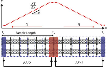
In the work reported here reversed nonequilibrium molecular dynamics (RNEMD)Reference Müller-Plathe19 is utilized to calculate both in-plane and out of plane thermal conductivity in the SWCNT-graphene superstructures by imposing a heat flux and measuring the induced temperature gradient (Fig. 1). The interactions between carbon atoms within SWCNTs and graphene are modeled using the AIREBO potential, which takes into account the bonding as well as nonbonding interactions among atoms. Within the AIREBO potential formulation, the potential energy of the system of atoms can be represented byReference Stuart, Tutein and Harrison20:
 $$E^{{\rm{AIREBO}}} = {1 \over 2}\mathop\sum\limits_i \,{\mathop\sum\limits_{j \ne i} {\left[ {E_{ij}^{{\rm{REBO}}} \!+ E_{ij}^{{\rm{LJ}}} \!+ \mathop\sum\limits_{k \ne i,j} {\mathop\sum\limits_{l \ne i,\,j,k} {E_{kijl}^{{\rm{tors}}} } } } \right]} ,}$$
Schematics of RNEMD. The sample length for thermal conductivity calculation is the half of the actual simulated structure.

where the reactive empirical bond order (REBO) potential,  $E_{ij}^{{\rm{REBO}}} $, describes the interactions between the covalently bonded atoms (the intramolecular interactions), while the dispersion and intermolecular repulsion interactions between the nonbonded atoms are accounted for through the use of the Lennard-Jones potential,
 $E_{ij}^{{\rm{LJ}}} $, term. The last term on the right-hand side of Eq. (1) accounts for the dihedral-angle intermolecular interactions, the contributions of which are generally deemed not significant in the analysis of CNTs.
To perform the MD simulations, first, the simulation box is divided into many bins along the direction in which the thermal conductivity is to be calculated. The middle bin of simulation box is chosen as the “hot bath” while the two end bins are chosen as the “cold baths.” During simulation, energy is swapped at each time step by exchanging velocity vectors of the coldest atom in the hot region and the hottest atom in the cold region to create a temperature gradient in the simulation structure.
The heat flux, q, from the cold region to the hot region due to the exchange of atoms can be expressed as:
 $$q = {1 \over {2tA}}\mathop\sum\limits_{{\rm{transfers}}} {{m \over 2}\left( {v_{\rm{h}}^2 - v_{\rm{c}}^2 } \right)} \quad.$$
In Eq. (2), v h is velocity of the hottest atom in the cold bath; v c is velocity of the coldest atom in the hot bath; m is mass of atom being swapped; A is the cross-sectional area perpendicular to the direction of heat flow; t is the total time over which the simulations are carried out; and the factor 2 in the denominator outside the summation sign arises because of the periodicity of the system.
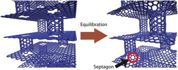
Figure 2 depicts the process of building SWCNT–graphene junctions in a typical pillared graphene unit cell. Such SWCNT–graphene junctions have previously been studied by Gonzalez et al.Reference Gonzalez, Guinea and Herrero21, Reference Gonzalez and Herrero22 from a geometrical perspective. Their work showed that only the (6n,0) zig-zag or (6n,6n) armchair nanotubes lead to regularly distributed septagonal carbon rings when combined with freestanding graphene layers. We chose a (6,6) armchair SWCNT for the present study. By manipulating the position vectors of a typical (6,6) SWCNT and a freestanding SLG sheet, a CNT end is brought in proximity of the dangling bonds of a precut matching hole in the graphene sheet so that they may be close enough to create covalent bonding. Next, the combined structure is equilibrated using MD to form SWCNT–graphene junctions each with six alternating hexagon–septagon ring pairs.
Formation of SWCNT–graphene junctions. Red circle mark indicates a septagon junction created after equilibration by MD.

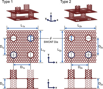
Each 3D superstructure utilizes either Type 1 or Type 2 unit cells as building blocks. Figure 3 shows the arrangement of the SWCNTs and graphene sheets in these two unit cells. The SWCNT pillars with faded lines represent pillars that are not in the same plane as the SWCNT pillars drawn with solid lines. As detailed in Table I, four different interpillar distances (Dx = 2.1, 2.5, 2.9, and 3.3 nm) and four different pillar heights (Dz = 1.2, 2.2, 3.2, and 4.2 nm) are chosen for this study. The 3D superstructures are built by repeating these unit cells along either the x-axis or the z-axis directions, which also correspond to the direction of thermal conductivity calculations. We refer to the thermal conductivity along the x direction (along the graphene layer) as the “in-plane” thermal conductivity, while the thermal conductivity in the z direction (i.e., along the CNT pillar axis) corresponds to the “out-of-plane” thermal conductivity. To obtain thermal conductivity of a superstructure with infinite size (infinite number of repeating unit cells), three different sizes of the 3D superstructure, for each unit cell type, are analyzed by repeating the unit cells 6, 10, and 20 times in the x and z directions. In addition, pristine (6,6) armchair SWCNT and pristine graphene structures with different structure sizes are also built and simulated to compare the thermal conductivity of the 3D superstructures with their base nanomaterials.
Type 1 and Type 2 unit cells used to build 3D superstructures. SWCNT pillars with faded lines represent pillars that are not in the same plane as the SWCNT pillars drawn with solid lines.

3D SWCNT–graphene superstructures analyzed in the present study.

Unit cell sides are determined by interpillar distances (L 1x = L 1y = 2D 1x, L 2x = L 2y = 2D 2x).
Both in-plane (along x) and out-of-plane (along z) thermal conductivities are calculated for each structure.
Total number of simulations are 192 [2 types × 4 interpillar distances × 4 pillar heights × 3 number of unit cells × 2 calculation modes (in-plane and out-of-plane)].
The large-scale atomic/molecular massively parallel simulator codeReference Plimpton23 LAMMPS, with the AIREBO interatomic potential is used in all simulations reported in the present work. First, the energy of the initial simulation structure is minimized to get a near 0 K temperature structure. Thereafter, time integration with isenthalpic (NPH) ensembles is performed with the Langevin thermostatReference Izaguirre, Catarello, Wozniak and Skeel24 at elevated temperature (500 K) for faster equilibration. Next, the simulation structure is cooled down to the room temperature and then equilibrated again with isothermal–isobaric (NPT) dynamics. RNEMD is performed on the equilibrated structures for 2 ns with microcanonical ensemble (NVE). All simulations show stable temperature profile after approximately 1 ns, which also confirms that our simulation time of approximately 2 ns used in RNEMD is sufficiently long for the thermal conductivity measurements.
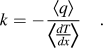
In view of Eq. (2), when heat flow in the structure reaches a steady state, averaging over the heat flux q, and temperature gradient dT/dx, and using the Fourier’s heat conduction law, the thermal conductivity, k, can be expressed as,Reference Bagri, Kim, Ruoff and Shenoy25
 $$k = - {{\left\langle q \right\rangle } \over {{\scale150%\langle} {{{dT} \over {dx}}} {\scale150%\right\rangle }}}}\quad.$$
The brackets  $\left\langle {} \right\rangle $in Eq. (3) indicates the average of the quantities over time as well as over the particles in the simulation cell.
The above approach, which has routinely been used in the past for computing thermal conductivity of homogeneous systems, can readily be applied to the 3D systems of interest in the present study. At planes coincident with the graphene layers at which the SWCNT–graphene junctions occur, the applied heat flux is expected to lead to a “jump” in temperature across the plane. This jump provides a measure of the boundary conductance, G (also known as the Kapitza conductance), of the graphene layers through the relation:
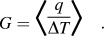 $$G = {\scale220%\langle} {{q \over {\Delta T}}} {\scale220%\rangle} \quad.$$
Furthermore, by appropriate selection of the heat flux direction, the temperature profiles that develop across the unit cells (in either the SWCNTs or graphene) can be analyzed to obtain the thermal conductivity in the out-of-plane and in-plane directions.
To present results of simulations for thermal conductivity in the 3D pillared graphene superstructures it is necessary to clearly define the cross-sectional areas due to significant spatial inhomogeneity (empty space) in these structures. One such cross-sectional area, perpendicular to heat flow, is the overall cross-sectional area of the pillared graphene system that includes the empty space. This area is most crucial from the perspective of utilization of these PGNs in engineering practice. Another important area consists only the region where the atoms are present, e.g., the area of the annular shell in CNTs. Such an area has been used in literature to calculate and predict thermal conductivity of CNTs and graphene and similar spatially nonhomogeneous systems at the molecular length scale. This area is also expected to be important in the study of phonon scattering in the PGNs and avoids nanotube length concerns on thermal conductivity, which would inherently appear if the former area was used.
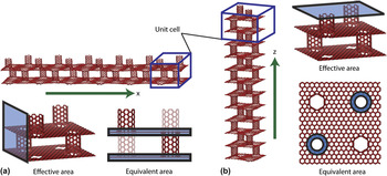
To address these issues, Figs. 4(a) and 4(b) show the cross-sectional area selections used in the present simulations for the calculation of the in-plane and the out-of-plane thermal conductivities, respectively, in the two types of 3D superstructures. The effective thermal conductivity (k eff) utilizes the area of the simulation box section perpendicular to the direction of thermal transport to calculate the thermal conductivity, while the equivalent thermal conductivity (k eq) considers the cross-sectional area of the path through which thermal transport occurs. Since the two graphene layers are the major contributors to in-plane thermal transport, the equivalent in-plane thermal conductivity calculation utilizes the cross-sectional areas of two graphene layers (of thickness 0.335 nm). On the other hand, the annular area of two SWCNTs (of thickness 0.335 nm) is selected for the calculation of the equivalent out-of-plane thermal conductivity since the two SWCNT pillars are the major paths for out-of-plane thermal transport.
3D superstructures with six repeats of Type 1 unit cell and schematics of cross-sectional area selection for (a) in-plane thermal conductivity measurement and (b) out-of-plane thermal conductivity measurement. Green arrows indicate the directions of thermal conductivity measurements. Shaded areas indicate the area used for thermal conductivity calculation.

III. RESULTS AND DISCUSSION
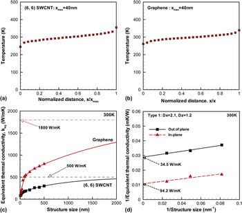
Before presenting the results for thermal transport in the 3D superstructures, we first validate our approach by computing thermal conductivity of defect-free (6,6) SWCNT and SLG. The temperature profile for a (6,6) SWCNT of length 40 nm is shown in Fig. 5(a). The total number of unit cells used in the simulation is 163, with each unit cell having 24 atoms. The computed temperature profile is nonlinear near the hot and cold ends due to finite size effects and also the high thermal conductivity of the SWCNTs, as also noted in previous works.Reference Bagri, Kim, Ruoff and Shenoy25, Reference Schelling, Phillpot and Keblinski26 Similar temperature profiles are also noted in SLG ribbon with overall dimensions of 40 nm in length and 4 nm in width (a total of 6520 atoms, with 2 atoms in each unit cell), as shown in Fig. 5(b).
(a) Representative temperature profiles of (6,6) SWCNT from RNEMD. (b) Representative temperature profile of graphene from RNEMD. The sizes of structures are normalized by their total structure sizes for easy comparison. (c) Approximation of thermal conductivity for infinitely large size of (6,6) SWCNT and graphene using empirical function. (d) Approximation of thermal conductivity for infinitely large size of 3D superstructures using the Matthiessen’s rule.

Care must be taken in extraction of thermal conductivity from this nonlinear profile, which indicates that thermal transport is not fully diffusive. To obtain the diffusive thermal conductivity, we consider the temperature gradient from the middle portion of the temperature profile (in between the thermostats). The thermal conductivity is found to be to depend on the size of the system. We find the thermal conductivity of (6,6) SWCNT with periodic lengths of 10, 25, 40, 60, 90, 120, 200, 300, 400, and 500 nm to be 80, 107, 145, 157, 174, 187, 209, 259, 269, and 299 W/(m K), respectively, while the thermal conductivity of SLG ribbons with periodic lengths of 10, 20, 30, 40, 60, 90, 120, 200, 300, 400, and 500 nm to be 73, 140, 181, 225, 427, 511, 545, 616, 693, 747, and 799 W/(m K), respectively. The dependence of the thermal conductivity on the length of the simulation cell can be understood by noting that the room temperature phonon mean free path of (6,6) armchair SWCNT and graphene (calculated by the simple kinetic theory) are 28 and 216 nm, respectively, which are larger than the size of our simulation unit cells. Therefore, in addition to phonon–phonon scattering, scattering at the heat baths (or boundaries) of the system influences the thermal conductivity of the sample.
On the basis of the kinetic theory of phonon transport, the thermal conductivity is proportional to the mean free path of phonon scattering. For the case in which the phonons scatter at the heat reservoir, the effective mean free path, l eff, can be expressed using the Matthiessen’s ruleReference Klemens27, Reference McGaughey and Jain28 as:
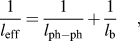 $${1 \over {l_{{\rm{eff}}} }} = {1 \over {l_{{\rm{ph}} - {\rm{ph}}} }} + {1 \over {l_{\rm{b}} }}\quad,$$
where l ph–ph is phonon–phonon scattering length and l b is the phonon–boundary scattering length (which is approximated to be sample length). Then, using Eq. (5) along with the kinetic theory of phonon transport, the thermal conductivity of the sample can be expressed as:
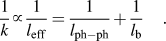 $${1 \over k} \propto {1 \over {l_{{\rm{eff}}} }} = {1 \over {l_{{\rm{ph}} - {\rm{ph}}} }} + {1 \over {l_{\rm{b}} }}\quad.$$
This relationship implies that the inverse of the thermal conductivity k, versus inverse of the system size l b, is a linear curve, and that the thermal conductivity for an infinitely large sample can be obtained by simple extrapolation, i.e., in the limit when  ${1 \over {l_{\rm{b}} }} \to 0$.
Figure 5(c) presents the variation of thermal conductivity with specimen size (length) for a 0.8 nm diameter SWCNT and a 4 nm wide graphene. From the data we observe that thermal conductivity transitions from being length dependent (i.e. ballistic thermal transport) to a regime where it approaches saturation, i.e., becomes length independent and is essentially diffusive. Although the extrapolation procedure [as described in Eqs. (5) and (6)] has been successfully applied to estimate thermal conductivity of 3D solid systems,Reference Schelling, Phillpot and Keblinski26, Reference Klemens27, Reference Ghosh, Calizo, Teweldebrhan, Pokatilov, Nika, Balandin, Bao, Miao and Lau29 the relationship between 1/k and 1/L for the SWCNTs under consideration in the present study is nonlinear, and a direct extrapolation to an infinite system length is therefore not possible.Reference Thomas, Iutzi and McGaughey30 We hypothesize that the primary reason for this breakdown of the linear extrapolation procedure is the assumption of a single phonon mean free path in the kinetic theory expression for thermal conductivity. This approximation, which assumes that every phonon travels the same distance on average before scattering, is poor for both CNTs and graphene, where the low frequency acoustic phonon modes have mean free paths several orders of magnitude larger than those of the other acoustic modes.Reference Donadio and Galli31
To quantify the transition from ballistic to diffusive phonon transport we fit the thermal conductivity data to the empirical function:
 $$k = k_\infty \left[ {1 - \left( {a\exp \left( { - {{l_{\rm{b}} } \over {l_{{\rm{c}}1} }}} \right) + b\exp \left( { - {{l_{\rm{b}} } \over {l_{{\rm{c}}2} }}} \right)} \right)} \right]\quad,$$
where  $k_\infty $ is the equilibrium diffusive thermal conductivity, l b is the sample length, l c1 and l c2 are critical lengths that describe the ballistic to diffusive transport transition, and a and b are constants, such that, a + b = 1. For the (6,6) SWCNT and the SLG analyzed in the present study, l c1 and l c2 are 25 and 900 nm and 65 and 2200 nm, respectively, with a = 0.3 and b= 0.7. Also, as shown in the plots, diffusive thermal conductivity in (6,6) SWCNT and SLG of infinite size are estimated to be ∼500 and 1800 W/(m K), respectively.
With regards to thermal conductivity of SWCNT, Berber et al.,Reference Berber, Kwon and Tomanek1 using nonequilibrium molecular dynamics (NEMD) with Tersoff potential, were the first to report a thermal conductivity of 6600 W/(m K) at room temperature. Since then, a large number of research groups, using MD, have reported thermal conductivity values that are consistently lower and with a large degree of scatter. Our estimate of 500 W/(m K) for the thermal conductivity of an infinitely large length (6,6) armchair SWCNT is lower than the Berber’s estimate but is consistent with the results of many other investigators. For example, MaruyamaReference Maruyama32 reported 350 W/(m K) as the thermal conductivity of (10,10) SWCNT with 100 nm length at 300 K using RNEMD with the Tersoff–Brenner potential. Osman and SrivastavaReference Osman and Srivastava33 also simulated (10,10) SWCNT using RNEMD but with the Tersoff potential and reported 1700 W/(m K) as the thermal conductivity of a (10,10) SWCNT with 22 nm length at room temperature. Padgett and Brenner,Reference Padgett and Brenner34 using RNEMD and a second generation REBO potential (which is very similar to AIREBO potential that we have used in the present work), reported 350 W/(m K) as the thermal conductivity of a (10,10) SWCNT with 350 nm length. Recently, Lindsay and BroidoReference Lindsay and Broido35 using a modified Brenner potential have reported a thermal conductivity of 2000 W/(m K) for a (10,10) SWCNT with 3 μm length; however, they reported 600 W/(m K) for a same length SWCNT using the original Tersoff potential. Experimental measurements of thermal conductivity in SWCNTs have generally been higher when compared to the theoretical predictions. For example, Pop et al.Reference Pop, Mann, Wang, Goodson and Dai3 reported 3500 W/(m K) as the thermal conductivity of SWCNT bundles at room temperature using an electrical self-heating method. Yu et al.Reference Yu, Shi, Yao, Li and Majumdar2 used a microheater to measure thermal conductivity of individual SWCNT and reported 3000–7000 W/(m K) as the thermal conductivity of individual SWCNTs.
Single layer graphene is understood to have a thermal conductivity that is higher than SWCNTs. However, as in the case of SWCNTs, there are disagreements in the theoretical predictions of thermal conductivity of SLG. Thermal conductivity of graphene was predicted to be between 8000 and 10,000 W/(m K) by Evans et al.,Reference Evans, Hu and Keblinski36 who used equilibrium MD with the Tersoff potential. Hu et al.Reference Hu, Ruan and Chen6 reported a thermal conductivity of ∼2000 W/(m K) at room temperature using RNEMD with the Brenner potential. Jauregui et al.Reference Jauregui, Yue, Sidorov, Hu, Yu, Lopez, Jalilian, Benjamin, Delkd, Wu, Liu, Wang, Jiang, Ruan, Bao, Pei, Chen, Srinivasan, Obeng, De-Gendt and Misra37 reported ∼1800 W/(m K) as the thermal conductivity of graphene at room temperature using NEMD simulation with the Brenner potential. Experimental predictions of thermal conductivity using the Raman optothermal methods have generally been higher than SWCNT for graphene. Balandin et al.Reference Balandin, Ghosh, Bao, Calizo, Teweldebrhan, Miao and Lau5 reported 2000–5000 W/(m K), while Jauregui et al.Reference Jauregui, Yue, Sidorov, Hu, Yu, Lopez, Jalilian, Benjamin, Delkd, Wu, Liu, Wang, Jiang, Ruan, Bao, Pei, Chen, Srinivasan, Obeng, De-Gendt and Misra37 reported 1500–5000 W/(m K) as the thermal conductivity of graphene using the Raman methods. However, more recently, much lower thermal conductivity values for graphene have been reported using experimental methods. Murali et al.Reference Murali, Yang, Brenner, Beck and Meindl38 reported 1100 W/(m K) as the thermal conductivity of graphene using the electrical self-heating method, while Seol et al.Reference Seol, Jo, Moore, Lindsay, Aitken, Pettes, Li, Yao, Huang, Broido, Mingo, Ruoff and Shi39 reported 600 W/(m K) as the thermal conductivity of graphene using two-probe electrical measurement.
Our MD results for the thermal conductivity of graphene of 1800 W/(m K) are supported in part by aforementioned theoretical calculations and experimental measurements. It is worthwhile to note that the thermal conductivities of carbon-based nanomaterials using RNEMD with second generation REBO or AIREBO potential have consistently been lower than those measured from experiments or those calculated using equilibrium MD. This is in contrast to the results obtained by the TersoffReference Tersoff40 potential, which is known to overestimate the thermal conductivity of graphitic materials.Reference Donadio and Galli41
Figure 5(d) shows results for in-plane and out-of-plane thermal conductivity obtained for three different superstructure sizes with Type 1 unit cells. Thermal conductivities of three different structure sizes are obtained by changing the number of repeating unit cells of the same size. In our present work, we used 6, 10, and 20 repeats of the Type 1 unit cell with Dx = 2.1 nm and Dz = 1.2 nm to generate the three superstructures. The plot of the inverse of the thermal conductivity as a function of the inverse of the size of the system [in Fig. 5(d)] confirms the linear relation. In accordance with Eq. (6), extrapolating the linearly fitted line to the y-axis with x= 0 provides an estimate of thermal conductivity for an infinite number of repeating unit cells (or an infinitely large structure size). Consequently, the in-plane and out-of-plane equivalent thermal conductivities for an infinite-sized superstructure are estimated to be 94.2 and 34.5 W/(m K), respectively.
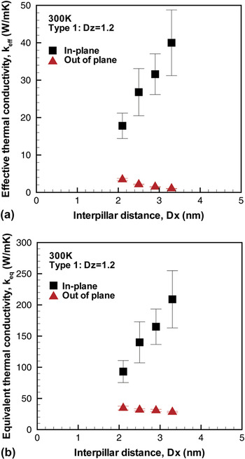
Using the aforementioned extrapolation procedure, in-plane as well as out-of-plane thermal conductivities for the 32 infinitely large superstructures with repeating Type 1 or Type 2 unit cells are reported. Figure 6 shows interpillar distance dependency of thermal conductivity of 3D superstructures with Type 1 unit cells. The in-plane thermal conductivity is expected to be affected by phonon scattering at the SWCNT–graphene junctions on the graphene floor in each unit cell; phonon scattering at these junctions scales with the ratio of the interpillar distance to the phonon mean free length in SLG. When this ratio is <1, the in-plane thermal conductivity on the graphene floors is expected to be ballistic.Reference Munoz, Lu and Yakobson42, Reference Saito, Nakamura and Natori43 However, as this ratio increases and crosses unity (with an increase in interpillar distance), phonon transport is expected to transit from ballistic (interpillar length dependent) to largely diffusive. Since the in-plane phonon transport in the superstructures we have analyzed is expected to be ballistic (due to their relatively small sizes), it leads to a near linear increase in thermal conductivity with an increase in inter pillar distance, as also observed from Figs. 6(a) and 6(b).
Unlike the in-plane thermal conductivity, the equivalent out-of-plane thermal conductivity is expected to depend weakly on the interpillar distance. This can be observed from Fig. 6(b), where the thermal conductivity decreases slightly with an increase in the interpillar distance. However, as depicted from Fig. 6(a), the effective out-of-plane thermal conductivity depends inversely on the square of the interpillar distance due to the increase in the cross-sectional area and hence is observed to decrease continuously as the interpillar distance is increased.
Thermal conductivity of 3D superstructures as a function of interpillar distance (Dx). (a) Effective thermal conductivity (k eff). (b) Equivalent thermal conductivity (k eq).

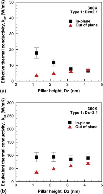
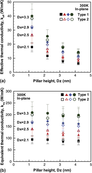
Figure 7 shows pillar height dependency of thermal conductivity of 3D superstructures with Type 1 unit cells. The increase in out-of-plane thermal conductivity with increasing pillar height can again be explained by the ballistic thermal transport in the SWCNTs.Reference Mingo and Broido44 Since the pillar heights of the unit cells used in the simulations are much smaller than the phonon mean free path in (6,6) SWCNTs, which is ∼28 nm (Fig. 5), the thermal conductivity of the SWCNTs is expected to increase with increasing lengths of the CNT pillars, thus increasing the effective and/or the equivalent out-of-plane thermal conductivity of the 3D superstructures. On the other hand, as observed from Fig. 7(b), the equivalent in-plane thermal transport is nearly unaffected by the increase in pillar height. This is to be expected since the increase in pillar height has a minimal influence on the in-plane phonon scattering by the presence of the junctions, which is understood to dominate the in-plane thermal transport. However, as inferred from Fig. 7(a), the effective in-plane thermal conductivity decreases with increasing pillar height. Again, this is to be expected since the increase in pillar height results in an increase in the cross-sectional area perpendicular to in-plane phonon transport, which is used in the in-plane thermal conductivity calculations.
Thermal conductivity of 3D superstructures as a function of pillar height (Dz). (a) Effective thermal conductivity (k eff). (b) Equivalent thermal conductivity (k eq).

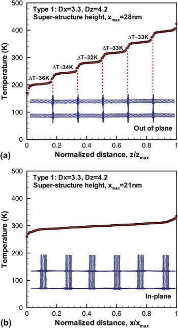
Figure 8(a) shows the temperature profile from the RNEMD simulations for out-of-plane thermal transport in the 3D superstructure with Type 1 unit cell with Dx = 3.3 nm and Dz = 4.2 nm. The temperature profiles are plotted as a function of the normalized superstructure height, z/z max, where z max is the height of the superstructure. From the plot, it can be seen that the position of the graphene layers (and the SWCNT–graphene junctions) correspond well with the location of the temperature jumps observed in the temperature profiles. For out-of-plane thermal transport the phonons must travel in the SWCNT pillars via the SWCNT–graphene junctions and then along the graphene layer in between to reach the next SWCNT pillar. In this regards, Lee et al.Reference Lee, Varshney, Brown, Roy and Farmer45 have investigated energy scattering of transverse and twisting acoustic modes as well as the radial breathing and flexural optical modes at the CNT–graphene junctions in a typical PGN. They showed that the geometrical arrangement of CNTs (pillars) and the intervening perpendicular graphene layer result in redistribution of the incoming phonon energy regardless of its direction. They also showed that low frequency phonon modes, which correspond to three acoustic modes and a flexural optical mode in the center of the Brillouin zone, experience strong reflections due to junction scattering. Since the low frequency phonon modes have mean free paths several orders of magnitude larger than those of other phonon modes,Reference Thomas, Iutzi and McGaughey30, Reference Donadio and Galli31 their scattering is understood to contribute largely to the observed decrease in the sample’s out of plane thermal conductivity. Moreover, the path taken by the phonons during out-of-plane thermal transport involves flow from one-dimensional (1D) (SWCNT) to two-dimensional (2D) (graphene) to again 1D (SWCNT) via the SWCNT–graphene junctions, which can contribute significantly to phonon dispersion due to the possible mismatch in phonon spectra at the junctions attributed to change in dimensionality, thus further increasing the complexity of out-of-plane phonon transport in these systems. Using Eq. (4), the average thermal conductance at the graphene floors in the superstructure can be estimated to be 1.46 × 10¹¹ W/(m2 K).
Representative temperature profiles from RNEMD simulations for (a) out-of-plane thermal transport and (b) in-plane thermal transport in 3D superstructures. Temperature jumps across graphene layers are calculated for out-of-plane thermal transport. The sizes of superstructures are normalized by total structure size for easy comparison.

Figure 8(b) shows the temperature profile for in-plane thermal transport in the 3D superstructure with Type 1 unit cell with Dx = 3.3 nm and Dz = 4.2 nm. It is interesting to note that the temperature jumps observed in the out-of-plane thermal transport are significantly smaller in the in-plane temperature profile. This implies that the thermal resistance, i.e., phonon dispersion and scattering at the SWCNT–graphene junctions on the graphene floors, for in-plane thermal transport is significantly smaller when compared with the out-of-plane thermal transport. This observation is also in agreement with the results presented in Figs. 6 and 7, which clearly indicate that the in-plane thermal conductivity is higher than the out-of-plane thermal conductivity for the cases analyzed in the present study.
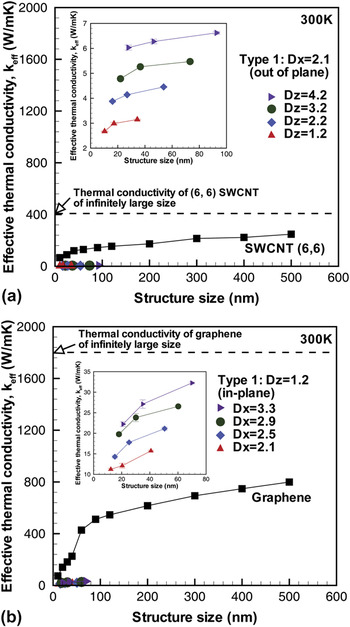
Figure 9 compares the thermal conductivity of the superstructure with their base nanomaterials, i.e., SWCNT and SLG ribbons. The 3D superstructures with Type 1 unit cells and with 2.1 nm interpillar distance (which exhibits the highest out-of-plane thermal conductivity among 3D superstructures simulated in our study) are chosen for the comparison with longitudinal thermal conductivity of (6,6) SWCNT in the axial direction [Fig. 9(a)]. On the other hand, the 3D superstructures with Type 1 unit cell and 1.2 nm pillar height (which showed the highest in-plane thermal conductivity) are chosen for comparison with thermal conductivity of pristine SLG [Fig. 9(b)]. As seen from Figs. 9(a) and 9(b), in all cases, the 3D superstructure displays significantly reduced thermal transport characteristics when compared with their base nanomaterials, i.e., SWCNT and single layer graphene. The highest effective out-of-plane thermal conductivity of 3D superstructure is 6.5 W/(m K) for a total structure size of 90 nm, while the effective thermal conductivity of (6,6) SWCNT is approximately 150 W/(m K) for the same size (length) structure. The highest effective in-plane thermal conductivity of 3D superstructure is 32 W/(m K) for 70-nm structure size, while the effective thermal conductivity of single layer graphene is about 250 W/(m K) for the same structure size. However, as discussed earlier, the 3D PGN structures, unlike the 1D CNTs and 2D graphene, are expected to contribute to both in-plane and out-of-plane thermal transport, simultaneously.
Comparison of 3D superstructures with their base nanomaterials. (a) Effective out-of-plane thermal conductivity of 3D superstructures and (6,6) SWCNT. (b) Effective in-plane thermal conductivity of 3D superstructures and single layer graphene. The insets are the zoomed-in plots of thermal conductivity of 3D superstructures.

Figure 10 compares the in-plane thermal conductivity of Type 1 and Type 2 superstructures. Both superstructures show very similar in-plane thermal transport characteristics. From the results, we can argue that the in-plane thermal transport is not sensitive to the arrangement of SWCNT pillars but only to the number of SWCNT–graphene junctions in a typical unit cell of the superstructure. The highest in-plane thermal conductivity is estimated to be 40 W/(m K) for the superstructure with Type 1 unit cell with the largest interpillar distance (3.3 nm) and the shortest pillar height (1.2 nm).
In-plane thermal conductivity of 3D superstructures with Type 1 and Type 2 unit cells as a function of pillar height. (a) Effective thermal conductivity (k eff). (b) Equivalent thermal conductivity (k eq).

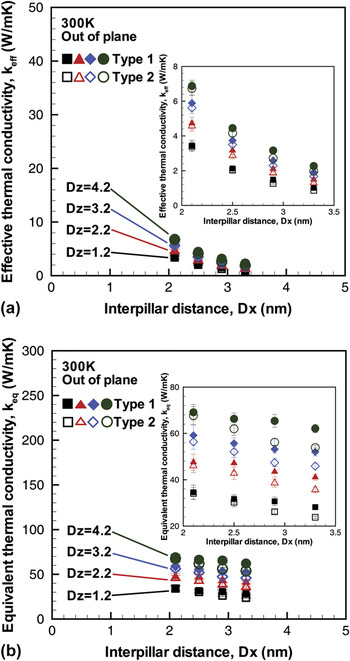
Figures 11(a) and 11(b) show the equivalent and effective out-of-plane thermal conductivities as a function of interpillar distance. The difference between Type 1 and Type 2 is more evident in the equivalent out-of-plane thermal conductivity plot [Fig. 11(b)]. Superstructures with Type 1 unit cell consistently show higher thermal conductivity when compared with the superstructure with Type 2 unit cells for all interpillar distances and pillar heights analyzed in the present study. During out-of-plane thermal transport, phonons traveling through the SWCNT pillars must also travel in the connecting graphene layer (in between the two pillars) before they move up to the next SWCNT pillar. Figure 12 shows the schematic of the two superstructures with Type 1 and Type 2 unit cells, respectively. In the superstructure with Type 1 unit cells, the SWCNT pillars are staggered, while in a superstructure with Type 2 unit cells, the SWCNT pillars are arranged essentially on one side. An interesting point of consideration in these structures is the shape of the equilibrated graphene floors and the resulting state of stress in the stretched graphene layer in the two architectures as a function of the interpillar distance. The shape of the graphene layer as well as the state of stress are expected to alter the wave speeds as well as phonon dispersion relations in graphene, and consequently both the in-plane and out-of-plane thermal transport in these structures, and will be the subject of detailed investigation of a future study. The highest effective out-of-plane thermal conductivity was observed to be 6.8 W/(m K) for the 3D superstructure with Type 1 unit cell with the smallest interpillar distance (2.1 nm) and the longest pillar height (4.2 nm).
Out-of-plane thermal conductivity of 3D superstructures with Type 1 and Type 2 unit cells as a function of interpillar distance. (a) Effective thermal conductivity (k eff). (b) Equivalent thermal conductivity (k eq). The insets are zoomed-in plots.

Unit cells during MD simulation. (a) Type 1 unit cell with Dx = 2.1 nm. (b) Type 2 unit cell with Dx = 2.1 nm.

IV. SUMMARY
In the present study, thermal transport in two different architectures of 3D pillared SWCNT–graphene superstructures is studied by investigating both in-plane and out-of-plane thermal conductivity using RNEMD with AIREBO interatomic potential. For the unit cells and 3D superstructures considered in the present study, it is found that the in-plane thermal conductivity increases linearly with an increase in the interpillar distance, indicating ballistic transport to be the major thermal transport mechanism in the in-plane direction. Moreover, the in-plane thermal transport in superstructures is insensitive to change in pillar height, while the effective in-plane thermal conductivity decreases with an increase in pillar height due to the increase in overall cross-sectional area of a typical unit cell. The out-of-plane thermal conductivity of the 3D superstructure is also found to increase linearly with an increase in pillar height, again indicating thermal transport to be largely ballistic in the out-of-plane direction in a typical unit sell. The equivalent out-of-plane thermal conductivity is weakly dependent on interpillar distance, while the effective out-of-plane thermal conductivity decreases with an increase in interpillar distance due to the overall increase in cross-sectional area.
The distinct temperature jumps in the out-of-plane temperature profiles obtained from the MD simulations indicate significant thermal resistance to phonon transport at the graphene floors (SWCNT–graphene junctions as well as the connecting graphene layer in between the junctions). On the other hand, it is interesting to note the absence of the temperature jumps at the SWCNT–graphene junctions in the in-plane temperature profiles indicating a much lower thermal resistance in the in-plane direction.
The results suggest that thermal transport in superstructures with Type 1 or Type 2 unit cell architectures is anisotropic with significantly lower out-of-plane thermal conductivity when compared to the in-plane thermal conductivity. Moreover, comparison of the out-of-plane and the in-plane thermal conductivity of 3D superstructures with SWCNT and SLG shows that the 3D superstructures have lower thermal transport properties when compared to their base nanomaterials due to scattering at the CNT–graphene junctions.
It was also identified that Type 1 unit cells displays a slightly high out-of-plane thermal conductivity when compared to Type 2 unit cells, but the in-plane thermal transport is largely unaffected by the pattern of SWCNT pillar arrangement.
ACKNOWLEDGMENT
The authors would like to acknowledge the support of the Air Force Office of Scientific Research (AFOSR) MURI Grant No. FA9550-12-1-0037 (Program Manager: Dr. Joycelyn Harrison) for conducting this research.