

1. Introduction
Land degradation and water shortages are major issues in developing countries, contributing to reduced economic output, lower growth potential and increased poverty. In Ethiopia, prevailing agricultural land use, advanced deforestation, mountainous terrain and seasonally heavy rainfall intensify land and watershed degradation, and may decrease agricultural productivity to unsustainable levels.
Over the last two decades, the Ethiopian government and a variety of development partners have invested in a myriad of sustainable land and watershed management (SLWM) programs. Thus far, most studies suggest that SLWM investments have a positive effect on agricultural output (Kassie et al., Reference Kassie, Pender, Yesuf, Kohlin, Bluffstone and Mulugetu2007; Holden et al., Reference Holden, Deininger and Ghebru2009; Olarinde et al., Reference Olarinde, Oduol, Binam, Diagne, Njuki and Adekunle2011); however, long-term maintenance of SLWM structures is not common among rural communities (Shiferaw and Holden, Reference Shiferaw and Holden1998; Tadesse and Belay, Reference Tadesse and Belay2004; WFP, 2005). Although previous studies have evaluated the impact of diverse technologies, no studies known to these authors have assessed the marginal effects of an extra year of sustained SLWM infrastructure on plot-level value of production in Ethiopia. This paper fills a critical knowledge gap by evaluating the time horizon to experience a significant impact given an investment in SLWM. Plot-level results suggest that terraces, bunds or check dams must be in place for at least seven years in order to have significant increases in the value of production.
Several matching techniques are used to ensure robust results. We use a nearest neighbor matching (NNM) technique developed by Abadie et al. (Reference Abadie, Drukker, Herr and Imbens2004) as well as kernel-based and radius matching in order to measure the impact of SLWM structures on value of production, understand how long SLWM structures must be in place in order to achieve a significant benefit, and calculate the marginal benefits of each additional year of maintenance.
The remainder of the paper is organized as follows. Section 2 provides a review of current literature on SLWM and its impact in Ethiopia and abroad. Section 3 describes the survey design and sampling strategy. Section 4 provides descriptive statistics by woreda (district), and treatment (plots that received SLWM investment) and control groups at the plot level. Section 5 discusses methodology and section 6 provides results. We summarize and conclude in section 7.
2. Background
Land degradation and poverty continue to challenge agricultural development opportunities in Ethiopia (Shiferaw and Holden, Reference Shiferaw and Holden2001; Zeleke and Hurni, Reference Zeleke and Hurni2001; Okumu et al., Reference Okumu, Jabbar, Colman, Russell, Barrett, Place and Aboud2002; Sonneveld, Reference Sonneveld2002; Tefera et al., Reference Tefera, Ayele, Atnafe, Jabbar and Dubale2002; Kassie et al., Reference Kassie, Holden, Köhlin and Bluffstone2008; Olarinde et al., Reference Olarinde, Oduol, Binam, Diagne, Njuki and Adekunle2011). Moreover, deforestation due to farmland expansion and energy needs, as well as fragile soils, undulating terrain and heavy seasonal rains make the highlands of Ethiopia highly vulnerable to soil erosion and gully formation. Under Ethiopia's previous five-year economic development plan (PASDEP: 2005–2010), the government invested in a series of land and watershed management activities with the goal of augmenting agricultural production. In the country's current five-year plan (Growth and Transformation Plan: 2010–2015), the government outlines the need to promote and invest in soil and water conservation activities (MoFED, 2010).
Given the demonstrable need for efficient mechanisms to improve water capture and agricultural output in the highlands, selected watersheds within the Blue Nile Basin in Ethiopia provide a good case study to test impacts of SLWM investment. Approximately two-thirds of the Blue Nile Basin is located in the more agriculturally productive highlands which receive relatively high levels of rainfall (800–2,200 mm per year). This area is dominated by cereal crops, which necessitate frequent soil mixing and provide very little ground cover during the long rainy season (meher rains), rendering it more susceptible to erosion (Werner, Reference Werner1986; Haileslassie et al., Reference Haileslassie, Priess, Veldkamp, Teketay and Lesschen2005).
According to previous studies, the on-site effects of land degradation (i.e., erosion and top soil loss), measured in lost agricultural production is estimated to cost 2–6.75 per cent of agricultural GDP per annum (Hurni, Reference Hurni1988; Bojö and Cassells, Reference Bojö and Cassells1995; Sonneveld, Reference Sonneveld2002). Holden and Shiferaw (Reference Holden, Shiferaw, Barrett, Place and Aboud2002) compared farmers’ perceptions of the costs of land degradation to an analysis using the universal soil loss equation to estimate the impact of soil erosion on overall crop yields. Results suggested that the average rates of land productivity decline were twice that of perceived rates, whereby 1.1 per cent of productivity is lost per year when no fertilizers are used, compared to 0.55 per cent loss per year when fertilizer application is efficient.
SLWM physical structures increase the value of production and agricultural yields through a variety of processes including: increased soil water content leading to extended crop growing periods; decreased erosion, ensuring important nutrients and inputs (topsoil, manure, fertilizer and seeds) remain on the plot; and decreased rainfall runoff volume preventing gully development and loss of agricultural area. Soil and water conservation measures including stone bunds, check dams and abandonment of post-harvest grazing in May ZegZeg catchment in north Ethiopia resulted in farmers planting crops in previously active gullies (Nyssen et al., Reference Nyssen, Clymans and Descheemaeker2010).
Previous research suggests that SLWM investments have a positive effect on productivity in Ethiopia. Pender and Gebremedhin (Reference Pender, Gebremedhin, Pender, Place and Ehui2006) and Holden et al. (Reference Holden, Deininger and Ghebru2009) found that plots with stone terraces experience higher crop yields in the Tigray region. SLWM has diverse effects depending on agricultural potential in Ethiopia (Kassie et al., Reference Kassie, Zikhali, Pender and Köhlin2010). Stone bunds and minimum tillage practices have higher returns in semi-arid and low agricultural potential areas respectively (Kassie et al., Reference Kassie, Pender, Yesuf, Kohlin, Bluffstone and Mulugetu2007, Reference Kassie, Zikhali, Pender and Köhlin2010). Similarly, Kato et al. (Reference Kato, Ringler, Yesuf and Bryan2011) found that SLWM infrastructure reaps positive and significant impacts on agricultural production in low rainfall areas in Ethiopia.
Studies outside of Ethiopia suggest similar results. A regional study in sub-Saharan Africa reported that households that invest in SLWM infrastructure achieve 17–24 per cent greater value of production compared to non-investing households (Olarinde et al., Reference Olarinde, Oduol, Binam, Diagne, Njuki and Adekunle2011). Increases in the value of production due to soil and water conservation programs were reported in Honduras (Bravo-Ureta et al., Reference Bravo-Ureta, Almeida, Solis and Inestroza2010). The PAES (natural resource management program) in El Salvador concluded that soil conservation technologies are positively correlated with farm income and length of time within the program (Cocchi and Bravo-Ureta, Reference Cocchi and Bravo-Ureta2007).
A majority of the studies on SLWM investments show a consistent pattern of costs exceeding benefits in the early years of SLWM investment, while improved agricultural yield in later years provides positive net returns. The analysis presented in this paper goes a step further to understand the timing of benefits and to conceptualize these benefits with the upfront and ongoing costs of investment and maintenance.
3. Survey design
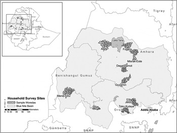
The household survey used for this analysis was completed in September 2010, and includes 1,810 households in nine woredas (districts), spatially distributed throughout the Blue Nile Basin (figure 1). A random sample was selected of approximately 200 households per woreda, and included households that: (1) were selected for an upcoming SLWM program, (2) had participated in any past SLWM program, and (3) had not participated in any past program. Heckman et al. (Reference Heckman, Ichimura and Todd1997, Reference Heckman, Ichimura and Todd1998) underline the importance of a comparable group of comparison observations, as well as comprehensive survey data that target characteristics correlated with the tested technology and outcome variables in order to assure reliable estimates. We stratified the household survey sample in order to allow for robust estimates of a single-difference in outcomes analysis.
Spatial distribution of survey sites

4. Household characteristics and perception of SLWM structures
In the sample villages, the most common public SLWM infrastructures focused on erosion mitigation and water conservation. Surveyed farmers reported that drought and excess rain affected 48 and 30 per cent, respectively, of farmers’ agricultural output. Stone terraces, soil bunds and check dams were ranked the most successful by 34, 29 and 11 per cent of households, respectively (see figure A1 in the online appendix available at http://journals.cambridge.org/EDE).
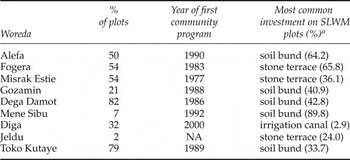
Private SLWM investments varied dramatically by woreda and by previous exposure to an SLWM program. For example, only 2 per cent of respondents from Jeldu woreda implemented SLWM activities on their own land (table 1).Footnote 1 However, 40 per cent of respondents in Jeldu identified erosion as a problem. Jeldu has received few SLWM support programs, and zero respondents worked on a previous public SLWM program (as compared to the sample average of 36 per cent participation). In comparison, 82 and 54 per cent of respondents in Dega Damot and Fogera, respectively, reported implementing SLWM on their private land, while 43 per cent of respondents in each woreda had also participated in a past community program.
Households using SLWM on private land

Source: Authors' calculations.
Notes: a We do not report drainage ditch because activity and definition varied dramatically by household.
Substantial diversity exists across woredas in terms of production patterns, agricultural activity and output prices, which has implications for income generation and production value. Within the sample, 64 per cent of farmers grow maize on a portion of their land, more than half of the farmers surveyed grow teff (55 per cent)Footnote 2 and over 40 per cent of farmers grow barley and wheat.
The mean value of production also varies dramatically by site. The Fogera (dedicates almost half of its area to teff production) and Diga (fertile maize production area) woredas enjoy relatively high values of production of 11,835 and 13,098 birr (US$845 and US$936) per household/year respectively.Footnote 3 However, due to a variety of constraints including high altitude, Dega Damot has a significantly lower value of production per household/year (approximately 5,000 birr or US$358), producing primarily barley, wheat and potato.
In addition, significant differences exist between households that invested SLWM on their plots compared to households that did not invest, such as age and education of household head, household size, as well as experience of a past drought (see appendix, table A1). Plot-level differences between investment and non-investment plots also vary. Plots that received SLWM investments have significantly less fertile soil, are located on steeper slopes and receive greater fertilizer inputs compared to non-investment plots.
Given that a variety of differences exist between plots that received investments and those that did not, we control for these potential underlying effects using a nearest neighbor and kernel-based matching approach. In addition, in order to quantify differences in value of production within investment plots given an extra year of sustaining SLWM infrastructure, we utilize a continuous treatment effects estimation.
5. Methodology
Three primary questions are explored in this paper. First, we assess the impact that SLWM has on the value of production for plots that receive an investment in comparison to matched plots with no investments. In doing so, we split the sample into plots that received early investments (plots that received SLWM infrastructure from 1992 to 2002) and late investments (2003–2009). Second, we estimate the marginal benefit (at plot level) of maintaining SLWM infrastructure from one year to the next. Finally, we construct a benefit cost analysis taking into consideration increased production due to investment and maintenance of SLWM in comparison to initial construction and ongoing labor costs.
In determining model specification, this research draws upon past theoretical frameworks of technology adoption. Characteristics of the adopter, biophysical features of the plot and type of SLWM infrastructure are important in explaining investment behavior. Pender et al. (Reference Pender, Place, Ehui, Pender, Place and Ehui2006) highlight that a series of plot- and household-level characteristics influence land management decisions. Additional variables such as access to technology, markets and information may influence income strategies and land management practices (Boserup, Reference Boserup1965; de Janvry et al., Reference de Janvry, Fafchamps and Sadoulet1991; Feder and Umali, Reference Feder and Umali1993). Adoption pathways are likely to be context specific (for example the NNM model described below takes into account differences in past experience with drought or floods, soil quality and hillside slope) and conditioned by microeconomic incentives at the household level. We take into account hypothesized determinants of investment based on previous theories of land management technology adoption in order to match investment plots to non-investment plots, while maintaining a balanced sample in order to ensure robustness of propensity score matching.
Nearest neighbor matching
In order to match plots that have SLWM infrastructure (treatment plots) with non-treatment plots (plots that did not receive SLWM), we first estimate a propensity score (or probability) of investment given observed characteristics. The sample is then balanced by calculating and verifying that the means of the observed distribution of covariates are similar for treatment and non-treatment plots. Individual treatment plots are then paired with non-treatment plots, as determined by a weighted average of the distance between values of the observed characteristic (allowing for five nearest neighbors in terms of absolute difference in propensity scores). Whereas NNM identifies a matching non-treated plot from the comparison group based on the closest propensity score to the treated plot, kernel matching uses weighted averages of all plots in the control group to construct a counterfactual outcome.Footnote 4
Once a balanced sample is achieved and trimmed (5 per cent of the sample from the top and bottom of the non-participant distribution is trimmed in order to assure comparisons over the same propensity score range), average outcomes of the treatment plots with the matched non-treatment plots are calculated and compared.Footnote 5 Thus, for each plot i, there are two potential outcomes: receive SLWM investment (treatment) or not receive SLWM investment (non-treatment). We denote treatment plots as A i (1) and non-treatment as A i (0), whereby the impact of investing in SLWM on the plot is the difference in outcome between treatment and non-treatment plots: Δ–A 1 − A 0. However, A 1 or A 0 for each plot is observed uniquely, given that the counterfactual is unknown. Thus, when D is an indicator variable equal to 1 if the plot receives SLWM investment and 0 if the plot does not receive SLWM, we find that the average impact of investment – the average impact of the treatment on the treated (ATT) – is defined as the following when X is a vector of control variables:
 $$\eqalign{ATT &= E\lpar \Delta \vert X\comma \; D = 1\rpar = E\lpar A_{1}-A_{0} \vert X\comma \; D = 1\rpar \cr &= E\lpar A_{1} \vert X\comma \; D = 1\rpar - E\lpar A_{0} \vert X\comma \; D = 1\rpar.}$$
In this case, impact is estimated by differences in total agricultural value of production between private plots with SLWM infrastructure investments and matched plots without SLWM. Results of these analyses are discussed in section 6.
Since the decision to invest in SLWM, as well as the length of time of maintenance may also depend on unobservable characteristics of plots or households, we test for the presence of hidden bias utilizing the Rosenbaum bounds sensitivity analysis (Rosenbaum and Ruben, Reference Rosenbaum and Ruben1983). Results suggest that there is no hidden bias due to an unobserved confounder within a factor of Γ = 2; thus an unobservable variable would have to cause more than a twofold difference in the odds, or twice as likely to receive an investment because of a difference in an unobserved variable. Previous research suggests that a twofold difference, given that plots are identical on matched covariates, is unlikely (Kassie et al., Reference Kassie, Zikhali, Pender and Köhlin2010; Keele, Reference Keele2010).
Dose-response and treatment effect estimates
When setting the model to estimate the effects of maintaining SLWM structures over time, we follow Hirano and Imbens (Reference Hirano, Imbens, Gelman and Meng2004) in their work on propensity score matching with continuous treatment effects. We consider a set of plots indexed by i where i = 1, …, N. Letting tϵT where t is the level of treatment defined as the number of years that soil bunds, terraces or check dams have been in place on specific plots, there is a certain level of potential outcome, Y(t), capturing the response to a level of treatment. In this case, the continuous treatment level t lies in the interval [t 0, t 1] and we define the potential outcome as the value of production per hectare for each plot. For each plot we observe the treatment level (number of years the plot has had an SLWM structure), the vector of covariates X i and the potential outcome corresponding to the received level of treatment. We then calculate the average dose-response function or the expected value of production given the number of years the plot is under SLWM, defined as:
 $$\mu\lpar t\rpar = E\left[Y_i\lpar t\rpar \right].$$
The key assumption set by Hirano and Imbens (Reference Hirano, Imbens, Gelman and Meng2004) generalizes the unconfoundedness assumption for binary treatments that, given a set of covariates explaining investment or no investment, treatment is random. In the continuous case, conditional on the set of covariate X’s, the extent of treatment is also random. Our identification assumption is that the number of years of maintaining SLWM is random, conditional on a set of plot and household characteristics.
Given that households adopted SLWM strategies in varying past years, the model should comprise covariates that would not have changed after adopting SLWM. We include total landholding size, biophysical characteristics of agricultural land such as soil quality and slope, and household head characteristics which are less likely to change over the study period. In order to further control for endogeneity, we do not match treatment and non-treatment plots based on household assets which may have been affected by successful or unsuccessful investments in SLWM (i.e., variables that proxy income).
When defining the generalized propensity score (GPS), let r(t, x) = f T/X (t, x) be the conditional density of the treatment given the covariates, then the GPS is R = r(T, X). As in the case of the binary propensity score, the GPS has a balancing property that ensures within each given strata (where the conditional density holds the same value), the probability that T = t does not depend on the covariates X.
The estimation of the dose-response function requires a computed conditional expectation of outcome as a function of the treatment level t and the GPS score R. The dose-response function at a particular t (level of treatment) is the conditional expectation over the GPS given by:
 $$\mu\lpar t\rpar = E\left[\beta\lpar t\comma \; r\lpar d\comma \; X\rpar \rpar \right] = E\left[Y\lpar T\rpar \right]\comma \; \hbox{where}$$
 $$\beta\lpar t\comma \; r\rpar = E\left[Y\vert T = t\comma \; R = r\rpar\right].$$
In order to successfully implement the above, a first-stage regression estimates the treatment level given the covariates:
 $$T_{i}\vert X_{i} \sim N \lpar \beta_0 + \beta_1^\prime Xi\comma \; \sigma^2\rpar.$$
In the simple normal model β0, β1 and σ2 can be estimated by maximum likelihood. The GPS is thus:
 $$\mathop {R_i} \limits^{\frown} = \displaystyle{{1} \over \sqrt{2 \pi\mathop {\sigma} \limits^{\frown}{}^2 }}\exp \left(-\displaystyle{{1} \over {2 \mathop {\sigma} \limits^{\frown}{}^2}}\lpar T_i-\mathop {\beta_0} \limits^{\frown}-\mathop{\beta_1^{\prime}} \limits^{\frown} X_i\rpar ^2\right).$$
In the second stage, the conditional expectation of Y i given T i and R i utilizes a quadratic approximation as suggested by Hirano and Imbens (Reference Hirano, Imbens, Gelman and Meng2004).
 $$E\left[Y_i\vert T_i\comma \; R_i\right] = \alpha_0+\alpha_1T_i + \alpha_2T_i^2 + \alpha_{3}R_{i} + \alpha_4R_i^2 + \alpha_5T_i R_i.$$
The parameters (α0, α1,…α5) are estimated using the calculated GPS R i by ordinary least squares. After estimating the second-stage parameter (see online appendix, table A2), the average potential outcome at treatment level t is predicted in order to obtain the entire dose-response function. Bootstrap methods are used to calculate more robust estimates, standard errors and confidence intervals. In the following section we provide greater detail of specific covariates and results for both the binary treatment and the continuous treatment effects.
6. Results
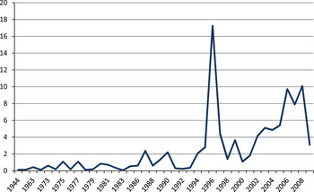
Propensity score matching is used in three separate analyses: impact of all investments from 1992 to 2009; early investments made from 1992 to 2002; and late investments from 2003 to 2009.Footnote 6 Plots that received early investments (1992–2002) and late investments (2003–2009) were selected based on spikes and drops in SLWM activity over the last two decades, as reflected in the data (figure 2). Although data exist on farmers implementing SLWM earlier than 1992, we evaluate from this year in order to not confound results with political upheaval and policy change that occurred during the Derg Regime (1974–1991). Second, less than 2 per cent of the total sample received structures prior to 1992, and less than 1 per cent of plots received SLWM investments in 1992. Each of the implementation periods requires separate NNM estimations at plot-level, but we maintain the same variables for each analysis, and in each analysis we maintain a balanced sample.
Percent of total plots under SLWM on private land (1944–2009)

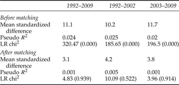
Matching results indicate that the common support condition is satisfied in the three analyses, which assures a comparable sample between plots that received investment (treatment) and those that did not receive SLWM investment (non-treatment). Evaluating the overlap in the distribution of the propensity scores of both treated and non-treated plots for the three analyses further suggests a comparable sample (online appendix, figure A2). In addition, when evaluating the distribution balancing of the variables included in the propensity score estimation, results show considerable reductions in the absolute standardized bias for the three analysis periods. Table 2 provides the results from the NNM covariate balancing tests before and after matching. The insignificant P values, as well as a low pseudo R 2 reported after matching, suggest that there is no systematic difference in the distribution of covariates between treatment and non-treatment plots.
Covariate balancing indicators from single NNM method

Source: Authors' calculations.
Correlates of adoption
The plot-level probit model used to match treatment and control plots reveals interesting information about investment choice on private land. It is important to note that causation cannot be attained from the probit regression, but rather these results suggest correlation with SLWM investment. The share of land characterized as non-fertile and on a steep slope is significantly different between treatment and control plots, suggesting that plots on steep slopes or semi-fertile and non-fertile land are correlated with SLWM investment on private land. In addition to biophysical constraints, households that experienced a past flood or erosion may be more inclined to invest in SLWM to insure against similar future occurrences (see appendix, table A1).
Impacts of adoption
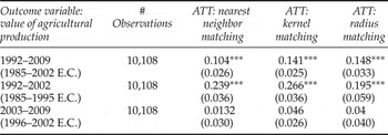
Results from plot-level NNM suggest that plots that received SLWM investments within the first period (1992–2002) experience a 24 per cent higher value of production in 2010 (table 3) compared to matched plots that did not receive SLWM. When analyzing plots that received SLWM investments in later years (2003–2009), there is no significant increase in the value of production. These results remain consistent when controlling for major crops (online appendix, table A3).Footnote 7 Unlike technologies such as fertilizer or improved seeds that immediately reap increased yields, benefits from constructing SLWM structures may accrue over longer time horizons. Nutrient and soil depletion is acute in areas of Ethiopia, and repletion is a multi-year process. Analysis suggests that SLWM infrastructure requires medium- to long-term investment to realize its designed effects (such as rebuilding the nutrients in the soil through decreased erosion, or improving and prolonging soil moisture processes through more efficient rainfall infiltration).
Average plot-level impact of SLWM adoption (single difference estimates)

Source: Authors' calculations.
Notes: ATT, average treatment effect on the treated; ***significance level at 1%; standard errors are in parentheses.
Next, we employ a continuous treatment effect analysis that allows a robustness check of impact by calculating the marginal effect of plot-level investment for each year the SLWM structure remains in place and functioning. Results echo the plot-level findings from the propensity score matching (PSM) of early investment whereby a structure must be in place for at least seven years to experience a significant increase in plot-level value of production.
Dose-response and continuous treatment effect estimation results
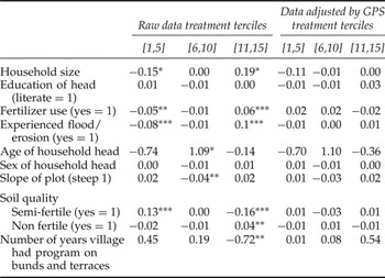
In order to better evaluate the marginal effects of SLWM adoption on private land, we employ a methodology of continuous treatment effect estimation as proposed by Hirano and Imbens (Reference Hirano, Imbens, Gelman and Meng2004). For the first-stage regression, we estimate the conditional distribution of the number of years an SLWM structure is maintained given a set of covariates (online appendix, table A4). We then divide the treatment distribution by treatment level whereby we define three intervals: [1,5], [6,10] and [11,15]. For each of these intervals, a group of observations is identified. There are 963, 563 and 603 observations in each group, respectively.
For each of the covariates used in the first regression, we then test and confirm that the mean of one group of observations is similar to the other two groups combined, and thus are able to satisfy the balancing property. Comparing the first three columns (raw data) in table 4 with the last three columns (adjusted by GPS), results suggest that the covariates are better balanced after the GPS adjustment. After balancing the covariates across the treatment intervals, the second-stage regression function is averaged over the GPS function at each level of treatment.Footnote 8
Test for equality of means between treatment groups (t-values)

Source: Authors' calculations.
Notes: GPS, generalized propensity score.
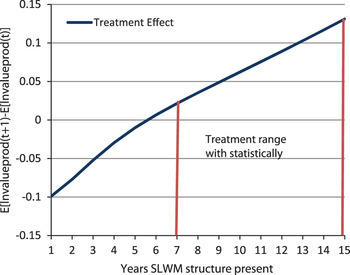
Analysis suggests that maintenance of SLWM is crucial to reap significant benefits. Adopters that maintain SLWM infrastructure for at least seven years see an increase in value of production at the end of the seventh year (figure 3). For adopters that have maintained their infrastructure less than seven years, there is no significant impact (the dose-response function, including confidence intervals, is presented in the online appendix, figure A3). This may be due to a variety of reasons. First, soil and water conservation structures slow degradation in the initial years of maintenance, but nutrient build-up from decreased erosion and runoff may take more time to show significant results on the value of production.
Marginal effect per extra year of maintenance

Previous studies suggest that agricultural yield improvements, given an SLWM investment, occur with some delay, and the initial investment costs exceed benefits in the early years of SLWM investment. A study examining soil degradation and nutrient repletion on smallholder farms in Kenya found that fallow land alone did not overcome nitrogen deficiency after eight seasons (Amadalo et al., Reference Amadalo, Jama, Niang, Noordin, Nyasimi, Place, Franzel and Beniest2003), but rather a mix of strategies including organic and inorganic fertilizer application, intercropping and fallowing were necessary. Ellis-Jones and Tengberg (Reference Ellis-Jones and Tengberg2000) evaluated stone and soil bunds in Kenya and found positive net returns after 10 years, assuming a productivity decline of 1.5 per cent per year on fields with no conservation structures. Shively (Reference Shively1999) reports similar results in the Philippines whereby positive net benefits of SLWM are experienced after six years of SLWM investment.
Not only is the marginal effect of adopting terraces, bunds or check dams positive, assuming maintenance for at least seven years, but the marginal benefit increases at an increasing rate. For example, if one sustains SLWM structures for seven to eight years, the value of production would increase by about 2 per cent, whereas if a household continues to maintain SLWM for 14–15 years the expected value of production increases by 12 per cent (figure 3). Although the marginal benefit increases with each additional year that the structure is maintained, this increase becomes statistically insignificant after 15 years. It is important to note, however, that there are minimal observations available for households that sustained SLWM for more than 12 years, and further investigation should be undertaken to understand the specific impacts of longer term maintenance. Assuming that nutrient repletion and erosion control is successful after long-term maintenance of SLWM structures, one would expect to see diminishing returns to such infrastructure as the necessary biophysical components are replaced.
Cost benefit
The PSM analysis suggests that most of the benefits from SLWM investments are realized only after seven years, which makes them especially sensitive to the choice of discount rate used in the cost benefit analysis. The most common procedure for dealing with uncertainty and risk is an increased discount rate; however, higher discount rates bias against long-term programs where benefits occur further in the future (Little and Mirrlees, Reference Little and Mirrlees1974). Following Stern (Reference Stern2007) we use a 3 per cent and a 5 per cent discount rate in order to construct the net present value (NPV) of increased agricultural production and the costs of initial SLWM investment and maintenance over time. The Stern review (Stern, Reference Stern2007) argues for a 5 per cent discount rate, hypothesizing alternative capital accumulation opportunities in the present without entirely discounting the welfare of future generations.Footnote 9 Weitzmann (Reference Weitzmann2007) suggests that individuals may be willing to pay for relatively safe stores of value that might represent ‘catastrophe insurance’, which would suggest the need for lower discount rates to invest in insurance now for future mitigation.
We assume a constant, real recurrent labor cost for yearly maintenance of structures at 516 birr per year (reported days and wage rate from the household survey). Given the off-season nature of SLWM work, we present estimates of labor costs using both the market wage for construction and maintenance of structures and a shadow wage rate of 50 per cent of the market wage.Footnote 10 The analysis assumes that, in the absence of adoption of SLWM technology, the value of production in previous years is equal to the 2009 level (in real terms). Finally, we use two scenarios of initial investment costs whereby construction of SLWM structures are fully subsidized, and construction costs are approximately four times (2,000 birr) that of annual upkeep.Footnote 11
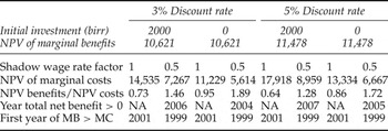
At a 5 per cent discount rate, the first scenario assumes a 2,000 birr initial investment. In this scenario, benefits outweigh costs beginning in 2007 and the benefit:cost ratio is 1.28, assuming a shadow wage rate factor of 50 per cent (table 5). With the same discount rate, and zero initial investment costs (households still incur annual labor costs for maintenance), benefits exceed costs in 2005 (benefit:cost ratio of 1.72). Using a 3 per cent discount rate, benefits outweigh costs in 2006 and 2004 for the two scenarios (2,000 birr and zero birr initial investment), respectively, and net benefits are 1.46 and 1.89 times that of costs. Thus, assuming an initial investment in 1992, the earliest that total benefits would exceed costs is 12 years later, even when the initial investment is fully subsidized.
Cost-benefit of investing in SLWM infrastructure (1992–2009)

Source: Authors' calculations.
Notes: NPV, net present value; MB, marginal benefits; MC, marginal costs.
These estimates are consistent with other cost-benefit studies found in the literature. Shiferaw and Holden (Reference Shiferaw and Holden2001) analyzed experimental trials of bunds and terraces in west and east Amhara and found insufficient economic incentives for investment in such structures. Hengsdijk et al. (Reference Hengsdijk, Meijerink and Mosugu2005) underlined the tradeoffs of investments in the Tigray region, whereby bunds slightly increased crop productivity during drier periods when yields were low, but decreased productivity during moist seasons because overall cropped area was reduced for the construction of bunds.
Regional differences exist, however. Gebremedhin et al. (Reference Gebremedhin, Swinton and Tilahun1999) estimated a 50 per cent rate of return on stone terraces based on experimental trials in the central Tigray region. Yitbarek et al. (Reference Yitbarek, Belliethathan and Stringer2010) implemented a more detailed cost-benefit analysis utilizing gully erosion costs and rehabilitation expenditure and benefits in four development projects in Amhara region and found that two of the four programs showed monetary gains after four and six years, respectively.
7. Conclusion
Prevailing agricultural land use, in combination with ongoing land degradation in the Ethiopian highlands, may reduce agricultural productivity to unsustainable levels. This paper uses household survey data from 2010 to explore three questions: what impact do SLWM investments have on the value of production? How long should SLWM infrastructure be in place to experience significant increases in the value of production? And what is the marginal benefit of keeping SLWM infrastructure in place from one year to the next? Finally, we construct a benefit cost analysis taking into consideration increased production due to investment and maintenance of SLWM in comparison to initial construction and ongoing labor costs.
Several techniques including NNM, kernel and radius matching are utilized to measure the impact of SLWM investment on private plots. Results suggest that terraces, bunds or check dams must be in place for at least seven years in order to have significant increases in value of production. Moreover, adopters that maintain the SLWM infrastructure for at least seven years see an increase in value of production at the end of the seventh year, with increasing marginal returns up to 15 years.
When taking into account construction costs and ongoing labor inputs, benefits do not outweigh costs until 12 years after SLWM construction (even when the initial investment is fully subsidized). Given the lagtime of positive net benefits, the assumed opportunity costs of labor and land, and the discount rate used to calculate NPV are very sensitive to profitability outcomes. Further research on seasonal labor and land use in the rural highlands, as well as how future environmental benefits are valued, will support policy and programs aiming to ensure sustainability. Understanding financing and incentive mechanisms for SLWM programs may be necessary to support longer term planning horizons.
This analysis suggests that long-term investment in SLWM is crucial. It is possible that the benefits and timing of SLWM could be improved through a more integrated approach of investments. Future research should evaluate the tradeoffs of a variety of investment packages (i.e., fertilizer and improved seed allocation in addition to SLWM investments). Moreover, market development and access is necessary to spur agricultural surplus, decrease transportation costs and improve distribution mechanisms of fertilizer and improved seed. These investments in tandem with SLWM measures may reap more sustainable benefits in the short and long run.
Supplementary materials and methods
The supplementary material referred to in this paper can be found online at journals.cambridge.org/EDE/.
Appendix
Plot-level probit: determinants of SLWM adoption 1992–2009