1. Introduction
The following process on a graph G was introduced by Aldous and Lanoue [Reference Aldous2]:
Initially, assign n real numbers
 $x_1,\ldots,x_n$
to the vertices of G. At each step uniformly at random select
 $\{i,j\}\in E(G)$
and replace both
 $x_i$
and
 $x_j$
with their average value
 $(x_i+x_j)/2$
.
As noted in [Reference Aldous2], this process was motivated by the study of social dynamics and interactive particle systems. Recently [Reference Chatterjee, Diaconis, Sly and Zhang6] further investigated this process in response to a question of Bourgain and a problem arising in quantum computing. In particular, sharper estimates for the rate of convergence were obtained for the case of G being a complete graph.
There are various procedures similar to the above process, such as the gossip algorithms studied in [Reference Shah16], the distributed consensus algorithms studied in [Reference Olshevsky and Tsitsiklis14], and various restricted averaging processes [Reference Acemoğlu, Como, Fagnani and Ozdaglar1, Reference Ben-Naim, Krapivsky and Redner3], as well as numerous ‘smoothing’ or ‘renewal’ models in statistics [Reference Chatterjee and Seneta7, Reference Feller11]. In addition, there are numerous random processes sharing similar flavors and methods, such as exchanging processes on permutations and card shuffling [Reference Diaconis and Saloff-Coste9].
In this paper we consider the following averaging process on a hypergraph H, and we emphasize that we place no restriction on the multiplicity or size of any edge of H.
Initially, assign n real numbers
 $x_1,\ldots,x_n$
to the vertices of H. At each step uniformly at random select an edge
 $e\in E(H)$
, and for each
 $i\in e$
replace
 $x_i$
with the average value
 $|e|^{-1}\sum_{j\in e} x_j$
.
Let us formalize this process somewhat. Recall that a hypergraph H is a set of vertices V(H) together with a multiset E(H) of subsets of V(H) which are called edges. Given a hypergraph H, let x be a real-valued vector indexed by V(H), which we call a weight vector of H. Define the (random) vector
 ${{\textrm{R}}_{H}^{}(x)}$
by choosing an edge e uniformly at random from E(H), and then setting
 ${{\textrm{R}}_{H}^{}(x)}_u=x_u$
if
 $u\notin e$
and
 ${{\textrm{R}}_{H}^{}(x)}_u=|e|^{-1}\sum_{v\in e} x_v$
otherwise. Recursively define
 ${{\textrm{R}}_{H}^{t}(x)} = {\textrm{R}}_{H}\big({{\textrm{R}}_{H}^{t-1}(x)}\big)$
. Equivalently,
 ${{\textrm{R}}_{H}^{t}(x)}$
is the random vector obtained by uniformly generating a sequence of t edges and then performing the averaging process for each edge sequentially. When H is understood, we simply write
 ${{\textrm{R}}_{}^{t}(x)}$
.
Given a weight vector x of H with
 $|V(H)|=n$
, we define the average vector
 $\overline{x}=\big(\frac{1}{n}\sum x_u,\ldots,\frac{1}{n}\sum x_u\big)$
. It is not too difficult to see (and we implicitly prove below) that if H is a connected hypergraph, then
 ${{\textrm{R}}_{H}^{t}(x)}$
converges to
 $\overline{x}$
as t tends to infinity for any weight vector x. The central problem we wish to consider is how quickly
 ${{\textrm{R}}_{H}^{t}(x)}$
converges to
 $\overline{x}$
in various norms.
It is well known that the rate of convergence of a simple random walk on a graph can be bounded in terms of the eigenvalues of the graph’s normalized Laplacian matrix; see, for example, [Reference Butler, Chung and Hogben5]. Analogous to this classical result, [Reference Aldous2] bounded the rate of convergence of the averaging process for graphs in terms of the second smallest eigenvalue of the (combinatorial) Laplacian. Motivated by this, we consider a Laplacian matrix for hypergraphs. In the literature there are many different definitions for Laplacians of hypergraphs [Reference Chung and Friedman8, Reference Feng12, Reference Lu and Peng13], and in this paper we use a definition introduced in [Reference Rodríguez15].
Given a hypergraph H, the codegree d(u,v) of two vertices
 $u\ne v$
is defined to be the number of edges e containing both u and v in H. If H is an n-vertex hypergraph, the codegree Laplacian L(H) is the
 $n\times n$
matrix with
 $L(H)_{u,v}=-d(u,v)$
if
 $u\ne v$
and
 $L(H)_{u,u}=\sum_{v\ne u} d(u,v)$
. For example, if
 $n=4$
and
 $E(H')=\{\{1,2\},\{1,2\},\{2,3,4\}\}$
, then
 \begin{equation*}L(H')= \left[\begin{array}{cccc} 2 & -2 & 0 & 0\\[3pt] -2 & \quad 4 & \quad -1 & \quad -1\\[3pt] 0 & \quad -1 & \quad 2 & \quad -1\\[3pt] 0 & \quad -1 & \quad -1 & \quad 2\end{array}\right].\end{equation*}
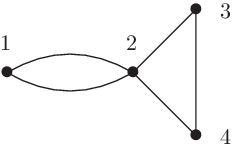
Note that when H is a graph this reduces to the Laplacian matrix of H. In fact, L(H) can be defined to be the Laplacian for the multi-graph
 $G_H$
obtained by placing a clique on all of the vertices of each
 $e\in E(H)$
. For example, with H
′ as above,
 $G_{H'}$
is the multi-graph displayed in Figure 1.
The multi-graph for the example hypergraph H.

While graphs G are uniquely determined by their Laplacian matrix L(G), we note that this is not true for hypergraphs. Thus, in general, passing from H to L(H) can throw out much of the combinatorial information about H.
1.1. Main results
It is clear that L(H) is a real symmetric matrix, and hence it has n real eigenvalues which we denote by
 $\lambda_0(H) \leq \lambda_1(H)\le \cdots\le \lambda_{n-1}(H)$
. It is not hard to show that
 $\lambda_0(H)=0$
with
 $(1,\ldots,1)$
a corresponding eigenvector, and that
 $\lambda_1(H)>0$
if and only if H is connected [Reference Rodríguez15]. With this in mind we can state our main result.
Theorem 1.1. Let H be a hypergraph with
 $|e|\le r$
for all
 $e\in E(H)$
. Then, for all weight vectors x and
 $t\ge 1$
,
 \begin{equation*}\mathbb{E}\left[\lVert{{{\textrm{R}}_{}^{t}(x)}-\overline{x}}\rVert_2^2\right]\le \left(1-\frac{\lambda_1(H)}{r|E(H)|}\right)^t\lVert{x-\overline{x}}\rVert_2^2.\end{equation*}
Note that the convergence in Theorem 1.1 becomes weaker as r increases. This is somewhat unintuitive since larger edges should allow for faster convergence. The saving grace is that larger edges typically imply that
 $|E(H)|$
is small, so in total the convergence often does improve as r increases; see, for example, Theorem 1.2.
We will show that Theorem 1.1 implies the following.
Corollary 1.1. Let H be a hypergraph on n vertices such that
 $|e|\le r$
for all
 $e\in E(H)$
. Then, for all weight vectors x and
 $t\ge 1$
, the iterated averaging process converges to its average value
 $\bar{x}$
as follows:
 \begin{align*} \mathbb{E}\left[\lVert{{{\textrm{R}}_{}^{t}(x)}-\overline{x}}\rVert_2\right]&\le\exp\left(\frac{-t\lambda_1(H)}{2r|E(H)|}\right)\lVert{x-\overline{x}}\rVert_2, \\[4pt] \mathbb{E}\left[\lVert{{{\textrm{R}}_{}^{t}(x)}-\overline{x}}\rVert_1\right]&\le \sqrt{n}\exp\left(\frac{-t\lambda_1(H)}{2r|E(H)|}\right)\lVert{x-\overline{x}}\rVert_2. \end{align*}
Thus, in expectation,
 ${{\textrm{R}}_{}^{t}(x)}$
is very close to
 $\overline{x}$
in the
 $L_2$
-norm whenever t is much larger than
 $2r|E(H)|/\lambda_1(H)$
, which is finite provided H is connected.
We can obtain concentration results for certain hypergraphs. To this end, a hypergraph H is said to be codegree regular if there exists some d with
 $d(u,v)=d$
for all
 $u\ne v$
. Examples of codegree regular hypergraphs include
 $K_n^{(r)}$
(the hypergraph on
 $\{1,\ldots,n\}$
with edge set consisting of every set of size r) and Steiner systems (hypergraphs where every pair is covered by exactly one edge). Also, recall that H is r-uniform if
 $|e|=r$
for all
 $e\in E(H)$
.
Theorem 1.2. Let H be an n-vertex r-uniform hypergraph which is codegree regular. Then, for all weight vectors x and
 $t\ge 1$
,
 \begin{equation} \mathbb{E}\left[\lVert{{{\textrm{R}}_{}^{t}(x)}-\overline{x}}\rVert_2^2\right]=\left(1-\frac{r-1}{n-1}\right)^t\lVert{x-\overline{x}}\rVert_2^2. \end{equation}
Moreover,
 $\lim_{t\to \infty} \lVert{{{\textrm{R}}_{}^{t}(x)}-\overline{x}}\rVert_2^2 \, \big / \left(1-\frac{r-1}{n-1}\right)^t$
exists and is finite almost surely.
Lastly, we note that the hypergraph averaging process can be used to model other averaging processes for which our results also apply. In particular, we define the neighborhood averaging process as follows. Let G be a simple graph and define the neighborhood
 $N_G(u)$
of a vertex
 $u\in V(G)$
to be the set of vertices adjacent to u in G. For x a weight vector of G, define the weight vector
 ${{\tilde{\textrm{R}}}_{G}^{}(x)}$
by uniformly at random selecting some
 $u\in V(G)$
, and then setting
 ${{\tilde{\textrm{R}}}_{G}^{}(x)}_v=x_v$
if
 $v\notin N_G(u)$
and
 ${{\tilde{\textrm{R}}}_{G}^{}(x)}_v=\frac{1}{|N_G(u)|}\sum_{w\in N_G(u)} x_w$
otherwise. We iteratively define
 ${{\tilde{\textrm{R}}}_{G}^{t}(x)} = {\tilde{\textrm{R}}}_{G} ({{\tilde{\textrm{R}}}_{G}^{t-1}(x))}$
, and denote this simply by
 ${{\tilde{\textrm{R}}}_{}^{t}(x)}$
whenever G is understood.
Theorem 1.3. Let G be an n-vertex d-regular graph and define
 $\lambda'\,:\!=\,\min\{\lambda_1(G),$
 $2d-\lambda_{n-1}(G)\}$
. Then, for all weight vectors x and
 $t\ge 1$
,
 \begin{equation*}\mathbb{E}\left[\lVert{{{\tilde{\textrm{R}}}_{}^{t}(x)}-\overline{x}}\rVert_2^2\right]\le\left(1-\frac{\lambda'(2d-\lambda')}{dn}\right)^t\lVert{x-\overline{x}}\rVert_2^2.\end{equation*}
From this, we can obtain bounds analogous to those of Corollary 1.1.
The rest of the paper is organized as follows. In Section 2 we prove some basic facts about the codegree Laplacian L(H). We then prove our main theorems in Section 3. We close the paper with a number of open problems and computational experiments in Section 4.
2. Preliminaries
In this section we state and prove several basic results about L(H), all of which are easy generalizations of the analogous results for graphs. To start, we show that the Raleigh quotient of L(H) has a particularly nice form. To simplify our lemmas, we adopt the convention that
 $\sum_{u,v}$
denotes the sums over all unordered pairs
 $\{u,v\}$
with
 $u\ne v$
.
Lemma 2.1. For
 $x\ne 0$
a real vector,
 $x^\top L(H)x=\sum_{u,v} d(u,v)(x_u-x_v)^2$
.
Proof. By definition, we have
 $(L(H)x)_u=\sum_{v\ne u} d(u,v)x_u-\sum_{v\ne u} d(u,v)x_v=\sum_{v\ne u} d(u,v)(x_u-x_v)$
. Thus,
 \begin{align*} \qquad\qquad\quad x^\top L(H) x & = \sum_{u} \sum_{v\ne u} d(u,v)(x_u^2-x_ux_v) \\ & = \sum_{u, v} d(u,v)(x_u^2+x_v^2-2x_ux_v) = \sum_{u, v} d(u,v)(x_u-x_v)^2. \qquad\qquad\qquad\square\end{align*}
We recall the following well-known linear algebra results, which can be found, for example, in [Reference Brouwer and Haemers4].
Lemma 2.2. ([Reference Brouwer and Haemers4]) Let M be a real
 $n\times n$
symmetric matrix. Then M has n real eigenvalues
 $\lambda_0\le \cdots \le \lambda_{n-1}$
, and
 \begin{equation*}\lambda_0=\min_{0\ne x\in \mathbb{R}^n} \frac{x^\top Mx}{x^\top x}.\end{equation*}
Further, any
 $x_0$
achieving this equality is an eigenvector corresponding to
 $\lambda_0$
, and
 \begin{equation*}\lambda_1=\min_{0\ne x\in \mathbb{R}^n:x\perp x_0}\frac{x^\top Mx}{x^\top x}.\end{equation*}
Putting these lemmas together gives the following.
Lemma 2.3. For all hypergraphs H,
 \begin{equation*}\lambda_1(H)=\min_{0\ne x\in \mathbb{R}^n:\sum x_v=0} \frac{\sum_{u,v} d(u,v)(x_u-x_v)^2}{\lVert{x}\rVert_2^2}.\end{equation*}
Proof. Because L(H) is real symmetric, we have from Lemmas 2.2 and 2.1 that
 $\lambda_0(H)$
is the minimum over non-zero real x of
 \begin{equation} \frac{\sum_{u, v} d(u,v)(x_u-x_v)^2}{\lVert{x}\rVert_2^2}. \end{equation}
Because the numerator and denominator of (2.1) are sums of squares,
 $\lambda_0(H)\ge 0$
. Moreover, by taking
 $x=(1,\ldots,1)$
we see that the minimum is exactly 0, and that the vector
 $(1,\ldots,1)$
is a corresponding eigenvector. By Lemma 2.2,
 $\lambda_1(H)$
is the minimum of (2.1) subject to
 $x\perp (1,\ldots,1)$
, i.e. subject to
 $\sum x_u=0$
.
Our main lemma gives a concise way of determining how much
 $\lVert{{{\textrm{R}}_{}^{}(x)}}\rVert_2^2$
differs from
 $\lVert{x}\rVert_2^2$
in expectation.
Lemma 2.4. For any weight vector x with
 $\sum x_u=0$
,
 \begin{equation*}\mathbb{E}\left[\lVert{x}\rVert_2^2-\lVert{{{\textrm{R}}_{}^{}(x)}}\rVert_2^2\right]=\frac{1}{|E(H)|}\sum_{e\in E(H)} \frac{1}{|e|}\sum_{u,v\in e} (x_u-x_v)^2.\end{equation*}
Proof. Assume the edge e is chosen in the averaging process. Then
 \begin{align*} \lVert{x}\rVert_2^2-\lVert{{{\textrm{R}}_{}^{}(x)}}\rVert_2^2 & = \left(\sum_{u\in e} x_u^2\right)-|e|\left(\frac{\sum_{v\in e} x_v}{|e|}\right)^2 \\ & =\frac{1}{|e|}\left(\sum_{u\in e} (|e|-1)x_u^2-2\sum_{u,v\in e}x_ux_v\right)=\frac{1}{|e|}\sum_{u,v\in e} (x_u-x_v)^2. \end{align*}
As each edge is equally likely to be chosen, we conclude the result.
3. Proofs of theorems
Let x
′ be a weight vector. It is not difficult to see that
 ${{\textrm{R}}_{}^{t}(x')}-\overline{x}'={{\textrm{R}}_{}^{t}(x'-\overline{x}')}$
, and an identical result holds for
 ${{\tilde{\textrm{R}}}_{}^{t}(x')}$
. Thus, it is enough to prove our results for
 $x\,:\!=\,x'-\overline{x}'$
. Throughout all of our proofs we assume x is a weight vector of this form, which means
 $\sum x_u=0$
and
 $\overline{x}=0$
.
Proof of Theorem 1.1. By Lemma 2.4 and the bound
 $|e|\le r$
,
 \begin{align*} \mathbb{E}\big[\lVert{x}\rVert_2^2-\lVert{{{\textrm{R}}_{}^{}(x)}}\rVert_2^2\big] & = \frac{1}{|E(H)|}\sum_{e\in E(H)}\frac{1}{|e|}\sum_{u,v\in e} (x_u-x_v)^2 \\ & \ge \frac{1}{r|E(H)|}\!\sum_{e\in E(H)}\sum_{u,v\in e}\!\!(x_u-x_v)^2=\frac{1}{r|E(H)|}\sum_{u, v}\! d(u,v)(x_u-x_v)^2. \end{align*}
By Lemma 2.3 this quantity is at least
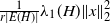 $\frac{1}{r|E(H)|}\lambda_1(H) \lVert{x}\rVert_2^2$
. By removing the determinstic value
 $\lVert{x}\rVert_2^2$
out of the expectation, we see that the result holds for
 $t=1$
, and the result in general follows by inductively applying the
 $t=1$
bound.
Proof of Corollary 1.1. For the first result we use
 $\mathbb{E}[X]\le \sqrt{\mathbb{E}[X^2]}$
, which is a consequence of Jensen’s inequality, Theorem 1.1, and the inequality
 $1-\tau\le \textrm{e}^{-\tau}$
, to conclude that
 \begin{align*} \mathbb{E}\left[\lVert{{{\textrm{R}}_{}^{t}(x)}}\rVert_2\right] & \le \sqrt{\mathbb{E}[\lVert{{{\textrm{R}}_{}^{t}(x)}}\rVert_2^2]} \\[4pt] & \le \left(1-\frac{\lambda_1(H)}{r|E(H)|}\right)^{t/2}\lVert{x}\rVert_2\le \exp\left(\frac{-t\lambda_1(H)}{2r|E(H)|}\right)\lVert{x}\rVert_2. \end{align*}
For the second result we use the Cauchy–Schwarz inequality and Theorem 1.1 to deduce that
 \begin{align*} \qquad\qquad\mathbb{E}\left[\lVert{{{\textrm{R}}_{}^{t}(x)}}\rVert_1\right] & \le \sqrt{\mathbb{E}\left[n\cdot \lVert{{{\textrm{R}}_{}^{t}(x)}}\rVert_2^2\right]} \\[4pt] & \le \sqrt{n}\left(1-\frac{\lambda_1(H)}{|E(H)|r}\right)^{t/2}\lVert{x}\rVert_2 \le \sqrt{n}\exp\left(\frac{-t\lambda_1(H)}{2r|E(H)|}\right)\lVert{x}\rVert_2. \qquad\qquad\square \end{align*}
For the proof of Theorem 1.3, we recall a basic fact from spectral graph theory. A walk of length k in a graph G is a sequence of (possibly not distinct) vertices
 $v_0,v_1,\ldots, v_k$
such that
 $v_i\sim v_{i+1}$
for all
 $0\le i<k$
. The following standard result can be found in [Reference Brouwer and Haemers4].
Lemma 3.1. ([Reference Brouwer and Haemers4]) Let
 $A(G)$
be the adjacency matrix of a graph. Then
 $A^k(G)_{u,v}$
is the number of walks of length k from u to v.
Proof of Theorem 1.3. Given a simple graph G, we define an auxiliary hypergraph
 $H_G$
by
 $V(H_G)=V(G)$
and
 $E(H_G)=\{N_G(u)\,:\,u\in V(G)\}$
. Observe that
 $H_G$
has n edges each of size d. It is not difficult to see that
 ${{\tilde{\textrm{R}}}_{G}^{t}(x)}$
and
 ${{\textrm{R}}_{H_G}^{t}(x)}$
have the same distribution, so by Theorem 1.1 we have
 \begin{equation} \mathbb{E}[\lVert{{{\tilde{\textrm{R}}}_{G}^{t}(x)}}\rVert_2^2]=\mathbb{E}[\lVert{{{\textrm{R}}_{H_G}^{t}(x)}}\rVert_2^2]\le \left(1-\frac{\lambda_1(H_G)}{dn}\right)^t \lVert{x}\rVert_2^2. \end{equation}
Note that for
 $u\ne v$
, the codegree d(u,v) in
 $H_G$
is equal to the number of common neighbors of u and v in G, which is exactly the number of walks of length 2 from u to v in G. Thus, by Lemma 3.1 we have
 $L(H_G)_{u,v}=-A^2(G)_{u,v}$
for
 $u\ne v$
and
 $L(H_G)_{u,u}=\sum_{v\ne u} A^2(G)_{u,v}=d^2-A^2(G)_{u,u}$
, where this last step used the fact that there are
 $d^2$
total walks of length 2 starting from u. We conclude that
 $L(H_G)=d^2I-A^2(G)$
. Because G is d-regular,
 $A(G)=dI-L(G)$
, and in particular the eigenvalues of
 $A^2(G)$
are exactly
 $(d-\lambda_i(G))^2$
. Thus, the eigenvalues of
 $L(H_G)$
will be
 $d^2-(d-\lambda_i(G))^2=\lambda_i(G)(2d-\lambda_i(G))$
. The smallest eigenvalue of
 $L(H_G)$
will be 0, corresponding to
 $i=0$
, and the second smallest eigenvalue will be
 $\min\{\lambda_1(G)(2d-\lambda_1(G)),\lambda_{n-1}(G)(2d-\lambda_{n-1}(G))\}=\lambda'(2d-\lambda')$
; this, together with (3.1), gives the result.
Lastly, we prove our result for codegree regular hypergraphs.
Proof of Theorem 1.2. Assume
 $d(u,v)=d$
for all
 $u\ne v$
. In this case
 $L(H)=dnI-dJ$
, where J is the matrix of all 1s. Thus, the vector
 $(1,\ldots,1)$
together with the
 $n-1$
vectors
 $(1,0,\ldots,0,-1,0,\ldots,0)$
form an orthogonal space of eigenvectors for L(H), with the latter eigenvectors all corresponding to the eigenvalue dn. In particular, every vector with
 $\sum x_u=0$
is an eigenvector corresponding to the eigenvalue dn. Using this with Lemmas 2.4 and 2.1 gives, for all x with
 $\sum x_u=0$
,
 \begin{align*} \mathbb{E}[\lVert{x}\rVert_2^2-\lVert{{{\textrm{R}}_{}^{}(x)}}\rVert_2^2] & = \frac{1}{r|E(H)|}\sum_{u\ne v} d(u,v)(x_u-x_v)^2 \\ & = \frac{1}{r|E(H)|}\cdot x^\top L(H)x=\frac{nd}{r|E(H)|}\lVert{x}\rVert_2^2. \end{align*}
Pulling out the deterministic value
 $\lVert{x}\rVert_2^2$
gives
 \begin{equation} \mathbb{E}\big[\lVert{{{\textrm{R}}_{}^{}(x)}}\rVert_2^2\big]=\left(1-\frac{nd}{r|E(H)|}\right)\lVert{x}\rVert_2^2. \end{equation}
To complete the proof of (1.1) when
 $t=1$
, we must show that
 $|E(H)|=\frac{n(n-1)d}{r(r-1)}$
. To do this, we count the pairs
 $(\{u,v\},e)$
with
 $u\ne v$
and
 $u,v\in e$
in two ways. We can first choose the pair
 $\{u,v\}$
in
 $\smash{\big({\scriptsize\begin{array}{c}n\\ 2\end{array}}\big)}$
ways and then the edge in d ways, or we could choose the edge first in
 $|E(H)|$
ways and then a pair it contains in
 $\smash{\big({\scriptsize\begin{array}{c}r\\ 2\end{array}}\big)}$
ways. This implies that
 $\smash{\smash{\big({\scriptsize\begin{array}{c}n\\ 2\end{array}}\big)} d=|E(H)|\smash{\big({\scriptsize\begin{array}{c}r\\ 2\end{array}}\big)}}$
, giving the desired result. The result for general t follows by inductively applying the
 $t=1$
case.
For the concentration result, define
 ${\textrm{S}}^t(x)=\big(1-\frac{r-1}{n-1}\big)^{-t}\cdot {{\textrm{R}}_{}^{t}(x)}$
, which in particular implies
 ${\textrm{S}}^t(x)=\big(1-\frac{r-1}{n-1}\big)^{-1}\cdot {{\textrm{R}}_{}^{}({\textrm{S}}^{t-1}(x))}$
. This, together with (3.2), implies
 \begin{equation*}\mathbb{E}\left[\lVert{{\textrm{S}}^t(x)}\rVert_2^2\ \big|\ \lVert{{\textrm{S}}^{t-1}(x)}\rVert_2^2\right]=\frac{\mathbb{E}\left[\lVert{{{\textrm{R}}_{}^{}({\textrm{S}}^{t-1}(x))}}\rVert_2^2\ \big|\ \lVert{{\textrm{S}}^{t-1}(x)}\rVert_2^2\right]}{\big(1-\frac{r-1}{n-1}\big)}=\lVert{{\textrm{S}}^{t-1}(x)}\rVert_2^2.\end{equation*}
Thus,
 $\lVert{{\textrm{S}}^t(x)}\rVert_2^2$
is a non-negative martingale, so its limit exists and is finite almost surely; see, for example, [Reference Durrett10, Theorem 4.2.12].
4. Concluding remarks
For ease of presentation, whenever H is understood we define
 $\Delta_1(t,x)=\lVert{{{\textrm{R}}_{H}^{t}(x)}-\overline{x}}\rVert_1$
. We write
 $f(n)\sim g(n)$
if
 $\lim_{n\to \infty} \frac{f(n)}{g(n)}=1$
, we write
 $f(n)=\Theta(g(n))$
if
 $\limsup\limits_{n\to \infty} \frac{f(n)}{g(n)}$
and
 $\liminf_{n\to \infty} \frac{f(n)}{g(n)}$
are positive constants, and we write
 $f(n)=o(g(n))$
if we have
 $\limsup_{n\to \infty} \frac{f(n)}{g(n)}=0$
.
The second half of Corollary 1.1 shows that
 $\mathbb{E}[\Delta_1(t,x)]\le c \lVert{x-\overline{x}}\rVert_2$
for some absolute constant
 $c<1$
whenever
 $t\ge Cr |E(H)|\log(n)/\lambda_1(H)$
for some
 $C>r$
. If H is the complete graph
 $K_n$
, then it is known that
 $\lambda_1(H)=n$
, so this happens when
 $t\ge Cn \log n$
for some
 $C>2$
. In particular, [Reference Chatterjee, Diaconis, Sly and Zhang6] shows that there exists x such that
 $\mathbb{E}[\Delta_1(t,x)]\sim \lVert{x-\overline{x}}\rVert_2$
if
 $t=o(n\log n)$
, so this shows that the bound of Corollary 1.1 is essentially tight (at least in terms of order of magnitude) when
 $H=K_n$
. This leads to the following (somewhat vague) question.
Question 4.1. When are the bounds in Corollary 1.1 essentially tight?
We give a concrete conjecture and question in this direction. Let
 $S_n$
be the star graph on
 $n+1$
vertices. Note that
 $|E(S_n)|=n$
and
 $\lambda_1(S_n)=1$
, so Corollary 1.1 shows that for any x we have
 $\mathbb{E}[\Delta_1(t,x)]\le c \lVert{x-\overline{x}}\rVert_2$
for some absolute constant
 $c<1$
whenever
 $t\ge Cn\log n$
for some
 $C>2$
. We suspect that this is tight.
Conjecture 4.1. Let x be the weight vector on
 $S_n$
which gives weight
 $1-\frac{1}{n+1}$
to the central vertex and weight
 $-\frac{1}{n+1}$
to every other vertex. Then, for
 $t=o(n\log n)$
we have
 $\mathbb{E}[\Delta_1(t,x)]\sim\lVert{x-\overline{x}}\rVert_2$
.
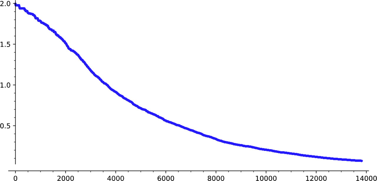
Figure 2 shows a plot of
 $\Delta_1(t,x)$
for this x and
 $S_{1000}$
. Note that in this case
 $2n\log(n)\approx 7000$
, and it does appear to take about this long for
 $\Delta_1(t,x)$
to start to decay.
 $\Delta_1(t,x)$
for
 $S_{1000}$
with
 $x_1=1-\frac{1}{1001}$
and
 $x_{i}=\frac{-1}{1001}$
for all other i.

On the other hand, we do not expect the bound of Corollary 1.1 to be tight for paths. If
 $P_n$
is the path graph on n vertices, then
 $\lambda_1(P_n)=2-2\cos(\pi/n)=\Theta(n^{-2})$
and Corollary 1.1 implies that
 $\mathbb{E}[\Delta_1(t,x)]\le c \lVert{x-\overline{x}}\rVert_2$
for some absolute constant
 $c<1$
whenever
 $t\ge Cn^3\log n$
for some
 $C>2$
.
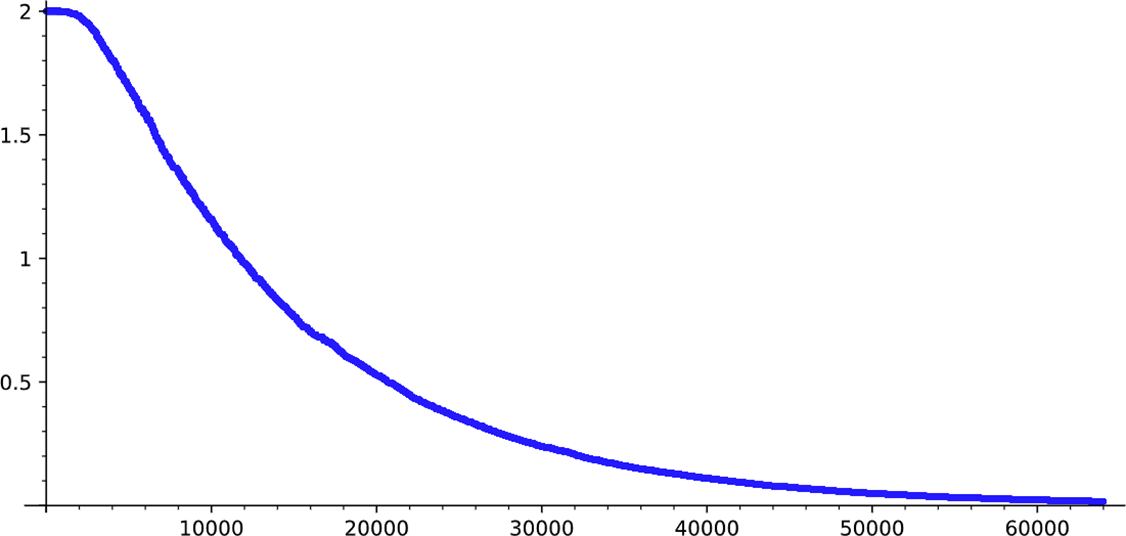
Figure 3 gives a plot of
 $\Delta_1(t,x)$
when x is the weight vector of
 $P_{40}$
taking the value
 $\pm 1$
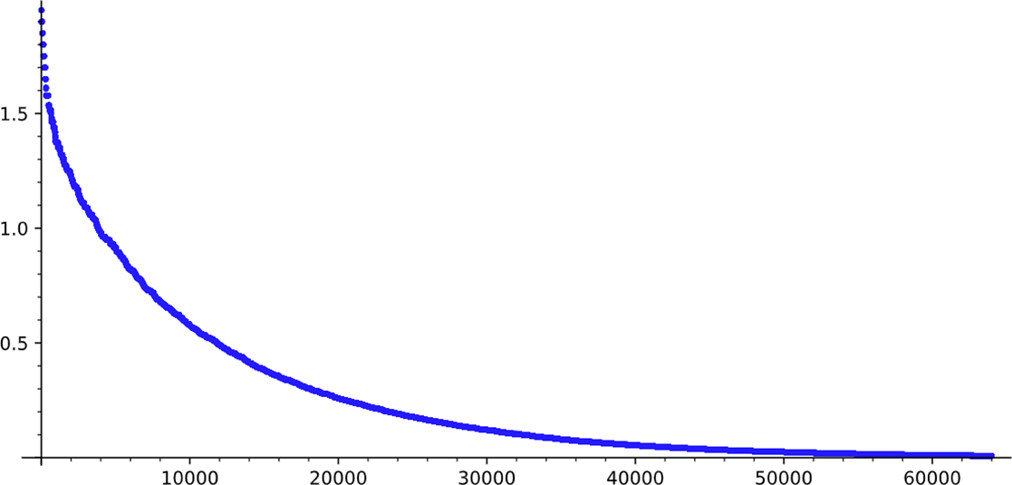
on each endpoint of the path and 0 everywhere else; Figure 4 shows a plot when x has weight
 $1-1/40$
on one endpoint and
 $-1/40$
on every vertex. Note that both processes seem to converge well within
 $n^3 = 64\,000$
steps. These results motivate us to suspect that the
 $\log n$
term in Corollary 1.1 is not necessary for the path.
 $\Delta_1(t,x)$
for
 $P_{40}$
with
 $x_1=1$
,
 $x_{40}=-1 $
, and 0 elsewhere.

 $\Delta_1(t,x)$
for
 $P_{40}$
with
 $x_1=1-\frac{1}{40}$
and
 $x_{i}=\frac{-1}{40}$
for all other i.

Question 4.2. For all
 $c>0$
, does there exists a constant
 $M=M(c)$
such that, for all weight vectors x of
 $P_n$
,
 $\mathbb{E}[\Delta_1(Mn^3,x)]\le \textrm{e}^{-c}\lVert{x-\overline{x}}\rVert_2$
?
We now turn our attention to the neighborhood averaging process. By adapting the proof of Theorem 1.3, we can obtain bounds on the convergence of
 ${{\tilde{\textrm{R}}}_{G}^{t}(x)}$
for all graphs G in terms of
 $\lambda_1(H_G)$
, where
 $H_G$
is the auxiliary hypergraph introduced in the proof of Theorem 1.3. Similar to how
 $\lambda_1(H)>0$
if and only if H is connected, we can show that
 $\lambda_1(H_G)>0$
if and only if G is connected and bipartite. From this, we can show that for a graph G, any weight vector x has
 ${{\tilde{\textrm{R}}}_{G}^{t}(x)}$
converging to
 $\overline{x}$
in expectation if and only if G is connected and nonbipartite.
Unfortunately, it is impossible to express
 $\lambda_1(H_G)$
in terms of
 $\lambda_i(G)$
for general graphs G. Indeed, it is well known that the eigenvalues of the Laplacian L(G) cannot detect whether G is bipartite in general, so in particular it cannot detect whether
 ${{\tilde{\textrm{R}}}_{G}^{t}(x)}$
will always converge to
 $\overline{x}$
. However, it may be possible to express
 $\lambda_1(H_G)$
in terms of eigenvalues of a different matrix associated to G. The most natural candidate would be the normalized Laplacian
 $\mathcal{L}(G)$
, since its eigenvalues can detect whether G is connected and bipartite in general; see the survey in [Reference Butler, Chung and Hogben5] for more on the normalized Laplacian. With this in mind we pose the following question.
Question 4.3. For any connected and not bipartite graph G, can we bound the convergence of
 ${{\tilde{\textrm{R}}}_{G}^{t}(x)}$
in terms of the eigenvalues of the normalized Laplacian matrix
 $\mathcal{L}(G)$
?
Acknowledgements
The author would like to thank Fan Chung for suggesting this problem. We thank her, as well as several anonymous referees and editors, for helpful comments on earlier drafts of this paper.
Funding Information
This material is based upon work supported by the National Science Foundation Graduate Research Fellowship under Grant No. DGE-1650112.
Competiting Interests
There were no competing interests to declare which arose during the preparation or publication process of this article.