


A substantial political economy literature argues that economic and fiscal reliance on petroleum, natural gas, and minerals helps create and perpetuate authoritarian political regimes. The genesis of this idea can be found in Mahdavy (Reference Mahdavy and Cook1970), who noted that petroleum revenues in Middle Eastern countries constituted an external source of rents directly captured by governments, thereby rendering them unaccountable to citizens. Other scholars then built upon Mahdavy (Reference Mahdavy and Cook1970) to postulate a general law about natural resource rents and authoritarianism. Luciani (Reference Luciani, Beblawi and Luciani1987), for example, avers that “The fact is that there is ‘no representation without taxation’ and there are no exceptions to this version of the rule.” Huntington (Reference Huntington1991, 65) then popularized this idea: “Oil revenues accrue to the state: they therefore increase the power of the state bureaucracy and, because they reduce or eliminate the need for taxation, they also reduce the need for the government to solicit the acquiescence of the public to taxation. The lower the level of taxation, the less reason for publics to demand representation.”
The idea that there is a causal relationship between natural resource reliance and authoritarianism underpins a broad and influential literature. This includes a plethora of country case studies, policy papers produced by multilateral aid organizations, popular books on world politics and economics, and articles in the mass media that make sweeping claims, such as the existence of a “first law of petropolitics” (Friedman Reference Friedman2006). The view that natural resources and democracy do not go together is often coupled with parallel literatures that find correlations between natural resources and slow economic growth or the onset of civil wars. Taken together, these literatures have given rise to the stylized fact that there is a “resource curse.”
Beginning with a seminal article by Ross (Reference Ross2001), numerous scholars have employed cross-country regression frameworks to examine the hypothesis that oil, gas, and minerals cause authoritarianism. Although the details vary, the vast majority of the literature produces results that are consistent with the hypothesis (e.g., Aslaksen Reference Aslaksen2010; Goldberg, Wibbels, and Myukiyehe Reference Goldberg, Wibbels and Myukiyehe2008; Jensen and Wantchekon Reference Jensen and Wantchekon2004; Papaioannou and Siourounis Reference Papaioannou and Siourounis2008; Ramsay n.d.; Ross Reference Ross2009; Smith Reference Smith2007; Wantchekon Reference Wantchekon2002). A considerably smaller literature either finds against the hypothesis (Herb Reference Herb2005), or finds that the effect of natural resources on regime type is conditional on other factors (Dunning Reference Dunning2008).
The researchers who find evidence that ostensibly supports the resource curse have not yet provided compelling tests of the hypothesis that natural resources cause authoritarianism. Neither, however, have the skeptics produced compelling results to the contrary. The fundamental issue is that the resource curse is about a dynamic process purported to unfold over time. Moreover, it requires the specification of a counterfactual: the discovery, production, and export of natural resources is hypothesized to distort a country's regime type, putting it on a different path of political development than it would otherwise have followed. The empirical tests that have been used to test the resource curse hypothesis, however, do not tend to employ time series–centric methods, nor specify counterfactual paths of political development. Instead, they tend to compare resource-reliant countries with resource-poor countries.
In using observational data, there is, of course, a big difference between finding a correlation between two variables and demonstrating that the relationship is causal. It is particularly problematic to infer causality when the correlation is produced by a technique that primarily exploits variance between countries. It would not take lengthy argumentation to demonstrate that there are fundamental differences between countries, and that these differences may be correlated with both the dependent and independent variables that researchers are introducing into their regressions. This is an inconvenient, but ubiquitous, feature of observational data. It implies that, unless a researcher is certain that the dependent and independent variables are uncorrelated with countries’ unobserved differences, it is not appropriate to estimate regressions that pool the data or employ random effects. There is a strong likelihood that the results generated by such approaches will be driven by omitted variables that are time-invariant and country-specific. The bottom line is this: when a process is hypothesized to occur over time, it is best to employ evidence and methods designed to see whether that time series process actually occurred.
This problem besets much of the resource curse literature. To put it concretely, the assumption behind the majority of the regressions in the literature is that, had Saudi Arabia not become oil-reliant, it might have developed the same political institutions as Denmark, provided that it had achieved the same per capita income and had fewer Muslims (see Ross Reference Ross2001). It is hard to believe, however, that endemic, time-invariant institutions that are not captured by covariates such as GDP per capita and the population share that is Muslim do not differentiate these countries. Moreover, these persistent, unspecified differences define the possible set of political institutions, and the possible set of economic sectors, that emerge and survive (Acemoglu et al. Reference Acemoglu, Johnson, Robinson and Yared2008). This includes the resource sector. As some researchers have pointed out, a country's resources, whether measured as stocks or flows, are not exogenous: they are determined by legal and cultural institutions (e.g., David and Wright Reference David and Wright1997; Norman Reference Norman2009).
Any number of factors might jointly determine resource reliance and authoritarianism. Permit us to provide just one example. Rulers who have inherited inveterately weak states tend to have pressing fiscal needs and short time horizons; they may therefore choose to search for resources and/or extract them at high rates today to obtain the rents needed for political survival, rather than save those resources for tomorrow. Indeed, as Manzano and Monaldi (Reference Manzano and Monaldi2008) point out, world oil reserves happen to be concentrated in precisely those countries with weak state capacity—and as any number of case studies have shown, weak state capacity preceded the discovery of oil or other minerals in those countries (e.g., Haber, Razo, and Maurer Reference Haber, Razo and Maurer2003). Given that countries’ underlying institutions are also correlated with their regime types (Acemoglu et al. Reference Acemoglu, Johnson, Robinson and Yared2008), it is likely that inveterately weak state capacity jointly determines authoritarianism and high levels of resource reliance.Footnote 1 Unfortunately, there is no consensus metric to operationalize “state capacity” across countries and time, let alone a metric that is exogenous. Moreover, there are likely to be several such unobserved factors that confound correlations between resource reliance and autocracy. The implication, we hope, is clear: lest the results be biased by omitted variables, time-invariant, country-specific factors have to be expunged.
A number of techniques are available to control for unobserved country heterogeneity, but one in particular—looking at variance within countries over time—gives researchers the flexibility to simultaneously address other factors that may also produce biased estimates. The core of our approach is to employ time series–centric methods that evaluate the long-run effect of resource reliance on regime types. We carry out this analysis using both a country-by-country time-series approach and a dynamic panel framework with country fixed effects. In order to do this, we construct original datasets whose time-series dimension extends back to the period before countries became reliant on natural resources: our panel covers 168 countries from 1800 to 2006. To ensure that our results are robust, we construct four different measures of natural resource reliance and employ the two most popular measures of regime type used in the literature.
We analyze the data with an eye to detecting and estimating time-series relationships, and do so by biasing in favor of the resource curse hypothesis. We diagnose the stationarity characteristics of both our resource reliance measures and regime type, and tend to find evidence that suggests that the data in levels are nonstationary. We therefore perform cointegration tests to see if there are grounds to suggest that there is a structural relationship between resources and regime types. When the tests suggest that we can reject the null hypothesis, implying a long-run relationship between these variables, we run error correction mechanism (ECM) regressions to estimate the direction, magnitude, and statistical significance of that relationship. However, because we want to bias our analysis in favor of the resource curse, and because there is always the possibility—however slight—that both unit root and cointegration tests can produce false negatives, we also run ECM models when we cannot reject the null of no cointegration. We do this to identify and report the direction of the relationship between resource reliance and regime types in levels, despite the fact that there are reasons to be dubious of any inferences that can be drawn from a regression in levels between two nonstationary and noncointegrated variables (Granger and Newbold Reference Granger and Newbold1974). That is, our goal is to leave no stone unturned in looking for evidence consistent with the hypothesis of a resource curse.
Focusing on the relationship between natural resource reliance and regime types within countries over the long run also allows us the flexibility to address other issues that may confound causal inference. For example, if there are good theoretical priors about factors that may condition the effect of an independent variable on the outcome of interest, the regressions need to go beyond simply estimating the average effect. Do natural resources always give rise to autocracy, or only under certain conditions? To answer this question we group countries by their level of income, inequality, threshold level of resource reliance, time period, and region, and then estimate separate regressions on those subsamples.
Another common problem in drawing causal inferences is the specification of the counterfactual outcome. What would have happened had a particular country not been exposed to the treatment variable of interest? One technique that researchers use to address this problem is a difference-in-differences estimator. Focusing on variance within countries over time also allows us to employ such an approach, but we differ from typical applications: we develop a technique that is suited to estimating the effect of a continuous treatment variable. First, we specify the counterfactual path that a resource-reliant country's regime type would have followed in the absence of those resources, on the basis of the path followed by the non–resource reliant countries in its geographic region. Second, we compare that counterfactual path with the actual path. Third, we see whether any divergence between the actual and counterfactual paths of political change correlates with increases in resource reliance. If one wanted, for example, to specify the counterfactual path that would have been followed by oil- and gas-rich Kazakhstan had it not discovered those resources, the best approximation would be the other Central Asian Republics that have not emerged as major resource producers (e.g., Uzbekistan)—but that share Kazakhstan's history of repeated invasions and occupations, as well as broad geographic and cultural characteristics.
Finally, researchers have to be certain that their results are not biased by reverse causality. Do natural resources fuel authoritarianism, or is it the other way around? Might it be the case that the only economic sectors that yield rates of return high enough to compensate for expropriation risk in authoritarian states are oil, gas, and minerals, thereby engendering resource reliance? We therefore create several instruments based on countries’ proven oil reserves that have both time-series and cross-sectional variance in order to estimate instrumental variables regressions with country fixed effects.
No matter how we look at the long-run data—including just making simple country-by-country graphs—we cannot find a systematic tendency that matches the concept of a resource curse. In fact, to the degree that we detect any statistically significant relationships, they point to a resource blessing: increases in natural resource income are associated with increases in democracy. This is particularly the case among countries that had low per capita incomes before they discovered resources. This is not to say that one cannot point to cases in which a dictator used resource rents to stay in power. It is to say, however, that there is a huge difference between identifying cases of a phenomena and making lawlike statements. The weight of the evidence indicates that scholars might want to reconsider the idea that there is a resource curse.
LITERATURE REVIEW
We are not the first researchers to have noted that the techniques employed in the resource curse literature may yield biased results. Indeed, resource curse researchers have become increasingly aware of the problems of drawing causal inferences from observational data.
Aslaksen (Reference Aslaksen2010) provides the best attempt to date to address unit heterogeneity bias by employing a dynamic panel model. Her approach, however, introduces a range of new problems. First, because the time dimension of her dataset (1972–2002) is only 30 years, she has to be concerned about Nickell Bias (correlation between the lagged dependent variable(s) and the unit fixed effects). She therefore employs a generalized method of moments (GMM) system approach. Her estimation strategy is to introduce a lagged dependent variable and a one-year lag of the independent variables, but this potentially imposes invalid restrictions on the structure of the data, thereby biasing the results (DeBoef and Keele Reference DeBoef and Keele2008). Second, although a system GMM estimator is designed to estimate models with data in levels that are highly persistent, this is not a license to neglect the evaluation of the time series properties of the data. In particular, Aslaksen does not evaluate whether her data are nonstationary—even though high persistence strongly suggests unit roots—and then take the proper steps to estimate relationships in light of this fact. Third, as Bun and Wendmeijer (Reference Bun and Wendmeijer2010) have shown, the system GMM estimator suffers from a weak instrument problem, making results unreliable. Finally, when estimating regressions that are centered on “within variance,” one has to be concerned about measurement error. Aslaksen potentially mitigates measurement error by abandoning yearly data as the unit of observation. She instead employs five-year averages. Unfortunately, by compressing the time dimension of the data into only six periods, Aslaksen foregoes the opportunity to model the time-series relationship between oil and democracy adequately.
Herb (Reference Herb2005) gains considerable traction on the specification of historically plausible counterfactuals for resource-reliant countries to better isolate the effect of resources on regime types. He reasons that resource-reliant countries would have been substantially poorer had they not found oil, gas, or minerals, and that their lower GDPs would have caused them to be less democratic. He therefore estimates what their GDP would have been in the absence of these resources, and then estimates their level of democracy at those lower, counterfactual levels of GDP. This is, however, only a partial solution: it ignores dynamics. A more powerful approach is to specify the alternative trajectories that resource-reliant countries would have followed in the absence of increasing resources, compare those counterfactual trajectories to their actual trajectories, and thereby control for other changes experienced by the resource-reliant cases during exposure to resources.
Dunning (Reference Dunning2008) provides the best attempt to date to address the possibility of conditional effects. He theorizes that when a society has a highly unequal distribution of income, natural resource wealth permits democratization because elites do not fear redistribution by the enfranchisement of the poor; conversely, when the distribution of income is more equal, natural resource wealth reinforces authoritarian regimes because leaders do not face demands for redistribution, and therefore can deploy the rents from resources to buy off or coerce opponents. He therefore introduces into the typical random-effects specification with resource reliance as the independent variable a measure of inequality and an interaction of inequality with resource reliance. These regressions, however, can be critiqued for employing a measure of inequality (the capital share of nonoil value added) that omits the oil sector. This potentially causes him to overestimate the share of income that is earned by labor in oil-rich countries that have undiversified economies (e.g., the Middle East). These regressions may therefore be picking up a fixed effect associated with undiversified oil economies. There are also other theoretically relevant conditional effects for which Dunning does not search.
Ramsay (n.d.) addresses endogeneity bias by instrumenting oil income with out-of-region natural disasters, reasoning that if a tsunami hits Malaysia, for example, it increases oil income in the rest of the world's producers without affecting their regime type through any other channel. Ramsay assumes that his instrument addresses both endogeneity and unobserved heterogeneity, and therefore does not introduce country fixed effects. This assumption is problematic. A short-term shock to oil prices will likely be offset by an immediate increase in oil production by a few big producers with substantial excess capacity before any increase in oil prices materializes. In fact, Saudi Arabia, the world's largest producer, seeks as a matter of policy to create a stable world oil market by manipulating output to offset shocks. In short, Ramsay's instrument may be picking up a “big producer” fixed effect—a conjecture supported by the fact that his instrument is rendered weak when the sample excludes the Middle East.
RESEARCH DESIGN
Measuring Regime Types
Our primary measure of regime type is the standard measure of democracy employed in the resource curse literature—the Combined Polity 2 score, an index of the competitiveness of political participation, the openness and competitiveness of executive recruitment, and the constraints on the chief executive that is coded for every country in the world from 1800 on (Marshall and Jaggers Reference Marshall and Jaggers2008). For simplicity, we refer to this measure as Polity. To make the regression coefficients easier to interpret, we normalize Polity to run from 0 to 100. Some researchers have argued that democracy is best measured as a binary variable. We thus also employ a widely used binary measure of democracy known as Regime (Przeworski et al. Reference Przeworski, Alvarez, Cheibub and Limongi2000) that we extend to run from 1800 to 2002. For a full discussion of the construction of this variable, as well as all of the other variables mentioned herein, see Online Appendix 1, Sources and Methods (available at www.journals.cambridge.org/psr2011001).
Measuring Oil and Mineral Dependence
Researchers have employed various measures of resource reliance in the extant literature. We draw upon those measures in undertaking our empirical analyses, but go beyond the extant literature in three ways. First, in order to be sure that our results are not driven by the choice of measure, we conduct our empirical analyses using four different measures. Second, the extant literature employs datasets that are truncated with respect to time: they typically go back no farther than 1970, with a few that extend back to 1960. We extend our measures back to independence or 1800 (if a country obtained independence before 1800). This means that we are able to observe countries before and after they became major natural resource producers. It also means that we are able to estimate the long-run effect of natural resources on a country's regime type. Third, rather than downloading datasets of uncertain provenance and quality that may be beset by measurement error, we construct our series from primary sources (when those are not available we give precedence to sources that are closest to the primary sources).
The resource curse literature claims that the causal mechanism that links natural resources to regime types is the rents captured by governments from oil, gas, and mineral production, which allow them to become “rentier states” that are financed without taxing citizens. We therefore follow Mahdavy (Reference Mahdavy and Cook1970) and Herb (Reference Herb2005) by constructing a measure of fiscal reliance on resource revenues, the percentage of government revenues from oil, gas, or minerals. For the sake of simplicity, we refer to this variable throughout the article as Fiscal Reliance. Unlike Mahdavy (Reference Mahdavy and Cook1970), who only covers a few years in the 1950s and 1960s for a small group of Mideast countries, and Herb (Reference Herb2005), who covers major producers during the period 1972–1999, we provide coverage of Fiscal Reliance from a country's first year of independence (or 1800) to 2006, allowing us to observe countries before and after they became oil, gas, or mineral producers.
There is one practical disadvantage to our time series approach to this measure: the retrieval and standardization of fiscal data extending back to the nineteenth century is not an enterprise characterized by economies of scale. We therefore truncate our coverage of Fiscal Reliance with respect to the number of countries by focusing on large producers that demonstrate variance in Polity (see Online Appendix 1, Sources and Methods, for details about the selection criteria). We code Fiscal Reliance for 18 countries: 16 oil and gas producers and 2 of the world's major copper producers. The oil and gas producers are Mexico, Venezuela, Ecuador, Trinidad and Tobago, Nigeria, Angola, Indonesia, Iran, Algeria, Bahrain, Equatorial Guinea, Gabon, Yemen, Oman, Kuwait, and Norway. The copper producers are Chile and Zambia.
We also estimate regressions on total oil income per capita (barrels produced, divided by population, multiplied by the real world price, expressed in thousands of 2007 dollars). For the sake of simplicity, we refer to this variable as Total Oil Income. Total Oil Income is a theoretically second-best metric compared to Fiscal Reliance: it measures the income earned by a country from crude oil, not the rents garnered by the government from that income. We employ it, however, for two reasons. First, it has emerged as the standard measure in recent work on the resource curse (e.g., Aslaksen Reference Aslaksen2010; Dunning Reference Dunning2008; Ramsay n.d.; and Ross Reference Ross2009). Second, it affords broad time series and cross-sectional coverage. Unlike the literature to date, however, which truncates coverage to the period since 1960, we begin coding in 1800 and cover 168 countries (104 display positive values) until 2006. Our first positive values are in 1861, just after the United States and Romania sank the world's first commercial oil wells.
We also develop two additional measures of resource reliance—Total Fuel Income (oil, natural gas, and coal, divided by population, expressed in thousands of 2007 dollars) and Total Resource Income (oil, natural gas, coal, precious metals, and industrial metals, divided by population, expressed in thousands of 2007 dollars). These measures are based on a measure frequently employed in the literature, the Hamilton and Clemens (Reference Hamilton and Clemens1999) Mineral Depletion variable (e.g., Aslaksen Reference Aslaksen2010; Dunning Reference Dunning2008). Our measures differ from theirs in multiple respects, the most salient of which is longitudinal coverage: we estimate our measures back to 1900, instead of 1960, as is standard in the literature.
Control Variables and Instrumental Variables
In the unrestricted specifications that follow we introduce a battery of variables to control for other determinants of regime type, such as per capita income, global and regional democratic diffusion effects, and civil war. We discuss those controls as we deploy them below. We also instrument for Total Oil Income with several measures based on oil reserves, which we discuss further below, to address reverse causation.
DATA ANALYSIS
Before diagnosing the time series properties of our data, and reviewing the results of several multivariate analyses, we first report some basic time series patterns adduced by inspecting and graphing the data for the 168 countries in our dataset. We hasten to emphasize that we are not drawing causal inferences from such a basic visual inspection of the data. Rather, this exercise is intended to provide readers with an idea of what the data look like in time series for each country, as well as to provide a preliminary grouping of the country series on the basis of whether a country appears to be blessed or cursed.
In order to bias in favor of uncovering patterns consistent with the resource curse hypothesis, we take two steps designed to exclude countries that are potentially resource-blessed. First, we decide whether a country is resource-reliant, based on its level of fiscal reliance on resource revenues. Poor, authoritarian governments often obtain significant revenues from natural resources, even if trivial quantities of those resources are produced in an absolute sense, whereas rich, democratic governments typically obtain trivial revenue shares from natural resources, even if large quantities of resources are produced. Second, we set the threshold for resource reliance at a relatively low level: an average of 5% during the period 1972–1999 (for the details see Online Appendix 1). This procedure yields a set of 53 resource-reliant countries. These criteria exclude resource-rich, mature democracies (e.g., the United States, Canada, Australia, and Great Britain), whereas they include authoritarian countries that produce trivial quantities of oil, gas, and minerals (such as Belarus, Tajikistan, and Morocco).
We summarize the patterns revealed after graphing the 53 country series for Polity, Total Resource Income, and Fiscal Reliance (when possible), across their entire histories, in Table 1. For reasons of space we are unable to reproduce all 53 graphs here. We do, however, present the graphs for the 18 countries for which we have data on both Fiscal Reliance and Total Resource Income (see Figures 1–18). We provide the graphs for the remaining countries in our dataset—the 35 other resource-reliant countries, as well as the 115 non–resource reliant countries—in Online Appendix 2, Data Analysis (available at www.journals.cambridge.org/psr2011001).
Patterns of Potential Resource Blessings and Curses

Note: Polity refers to normalized combined Polity score (0 to 100).
Norway

Trinidad and Tobago

Venezuela

Ecuador

Mexico

Algeria

Angola

Iran

Indonesia

Zambia

Chile

Nigeria

Bahrain

Equatorial Guinea

Gabon

Kuwait

Oman

Yemen

Potential Resource Blessings
Nineteen of the 53 resource-reliant countries appear to have been blessed by increases in resource reliance. Six countries remained democratic after they experienced resource booms, where democratic means that Polity is 85 or above, following Jaggers and Gurr (Reference Jaggers and Gurr1995). Seven countries transitioned to democracy during or after resource booms. Two countries were near-democracies (Polity was 80) before resource booms, and remained at that level during the booms. Four countries were autocracies before they had resource booms, and although they did not reach the threshold for democracy, they had at least one–standard deviation increases in Polity (25 points, based on the data's “within” variation) during or after those booms.
Let us begin with the cases in which a democratic country experienced an oil boom and remained democratic. Norway (Figure 1) is a well-known case that is usually thought of as an exception to the resource curse, but less well known is the experience of Trinidad and Tobago (Figure 2). Trinidad and Tobago was democratic at independence in 1962, and even though Fiscal Reliance and Total Resource Income increased dramatically in subsequent years—indeed, Trinidad has one of the highest levels of Resource Income Per Capita in the world—Polity continued to tick upward, reaching the maximum score of 100 in the 1990s.
Three of the graphs display data consistent with democratization during a resource boom. Venezuela (Figure 3) has been written about extensively, but other cases, such as Ecuador (Figure 4) and Mexico (Figure 5), are less well known. Mexico is a particularly critical case, because it had two distinct resource booms, punctuated by a long period of decline and stagnation of its oil and mineral sectors: the first boom ran from 1900 to 1924, whereas the second boom has been ongoing since 1974. Mexico's first resource boom ended after it had exhausted its oil reserves, given the technology of the time (Haber, Razo, and Maurer Reference Haber, Razo and Maurer2003), but Polity did not increase in the wake of this resource bust, as predicted by the theory of the resource curse. Instead, Mexico saw the heyday of single–party rule. Mexico's second resource boom also did not produce the political outcome predicted by the resource curse: as oil rents increased, the Partido Revolucionario Institucional (PRI) gradually lost its viselike grip on power. In 2000, when the PRI finally lost control of the presidency, Fiscal Reliance was four times its 1960s level (23%, as compared to roughly 6%), whereas Total Resource Income had increased sixfold, to $478 per capita. In 2006, when Mexico held a second free and fair election, Fiscal Reliance and Total Resource Income were even higher: 37% and $871 per person, respectively.
An additional three graphs display cases in which Polity increased by at least one standard deviation during a resource boom: Algeria (Figure 6); Angola (Figure 7); and Iran (Figure 8). As is well known, none of these countries ever became democratic. Nevertheless, they do not display the patterns that one would expect, given their reputations as being resource-cursed. Iran is a particularly striking example (see Figure 8). When the Shah came to power in 1941, Iran was a trivial producer of petroleum and the government obtained less than 1% of its revenues from natural resources—hardly the “rentier state” that one might imagine from the case that inspired Madhavy's (Reference Mahdavy and Cook1970) theory. Conversely, it was when income from natural resources and fiscal reliance were at all-time highs, in the late 1970s, that Iranian civil society mobilized against the Shah's repressive dictatorship and overthrew it. In the decade leading up to the 1979 Revolution, Total Resource Income averaged $1,999, whereas Fiscal Reliance averaged 66%. Even more striking, during the period in which Ayatollah Khomeini crushed the revolution's progressive elements and constructed an Islamic theocracy, Total Resource Income and Fiscal Reliance on that income had collapsed: during the period 1980–1989, Total Resource Income averaged only $894—less than half of its 1970s level—and Fiscal Reliance on that income had fallen as well, to 52%.
Potential Resource Curses
A case can be made for a potential resource curse on the basis of the graphed data in only 8 of the 53 countries, which is surprising, given the generous criteria we have employed to capture the set of resource-reliant countries. Two cases democratized after their resource booms collapsed: Bolivia and Indonesia (Figure 9). In an additional four cases, Polity increased by one standard deviation after the collapse of a resource boom: the Democratic Republic of the Congo, Guinea, Liberia, and Zambia (Figure 10). Of these, Zambia, which at one time was a major copper producer, perhaps makes the strongest case: although it was autocratic during the heyday of its copper production in the 1960s and early 1970s, its fiscal reliance on copper steadily declined from a peak of over 50% to 6% by 1991, at which time its Polity score increased 16-fold. There is only one case in which democracy failed during or after a resource boom (Belarus), as well as only one case in which Polity declined by at least one standard deviation during or after a resource boom (Congo). In short, potentially resource-blessed countries outnumber potentially resource-cursed countries by a ratio of more than two to one.
One might object that this ratio might be driven by the fact that our criteria for selection into the group of 53 resource-reliant countries allow a number of trivial producers to be included in the potentially blessed set. Lithuania, Kyrgyzstan, and Niger all produced less than $100 on average in Total Resource Income (the mean is $595 for all 168 countries, including those that produce no natural resources at all). By that same standard, however, we would also have to exclude three of the eight potentially resource-cursed countries (Belarus, Guinea, and the Democratic Republic of the Congo). The ratio of potentially resource-blessed to potentially resource-cursed countries would therefore increase: to more than three to one.
What are we to make of the remaining 26 cases? Seven are inconclusive: either they display no discernable pattern, such as in Chile and Nigeria (Figures 11 and 12, respectively), or substantial movements in Polity precede movements in Total Resource Income. The remaining 19 are cases that were autocratic prior to the discovery of natural resources, and remained autocratic after they experienced resource booms. They also failed to democratize in the wake of the collapse of their resource incomes in the 1980s and 1990s. We graph the series for six cases for which we have data on both Fiscal Reliance and Total Resource Income: Bahrain (Figure 13), Equatorial Guinea (Figure 14), Gabon (Figure 15), Kuwait (Figure 16), Oman (Figure 17), and Yemen (Figure 18). The most reasonable interpretation of these 19 cases is that natural resources and authoritarianism are unrelated.
In keeping with our goal of biasing in favor of uncovering patterns consistent with a resource curse, we would like to argue that these 19 countries would have democratized in the absence of oil and mineral reliance. In order to do so, however, we would have to set aside three inconvenient facts about them: (1) they are clustered in two geographic areas of the world; (2) they have long legacies of authoritarianism that antedate their oil discoveries; (3) the non–oil producing countries of those world areas also have long-lived authoritarian states. Twelve of the 19 cases are clustered in the Middle East and North Africa (MENA), a region that has a long history of tribal social organization, foreign conquest (beginning with the Sassanid Empire, followed by the Ottomans, and ending with British protectorates), and authoritarian government. Virtually all had been kingdoms, sheikdoms, or imamates for centuries before they found oil. Moreover, their neighbors, Jordan and Syria, share these same historical legacies, but importantly not their natural resource wealth—and they are not democracies either. This suggests that resources were not the decisive factor shaping the political trajectories of the other 12. A similar pattern holds if we posit Yemen as the appropriate comparison: prior to its discovery of (quite modest amounts of) oil in 1980 it too was a long-lived autocracy. Much the same is true of three cases that are clustered in the former Soviet States of Central Asia (Kazakhstan, Turkmenistan, and Tajikistan). In fact, until they were absorbed into the Russian Empire in the nineteenth century, they were populated by tribal peoples who were not organized into territorial states. They therefore have a legacy of authoritarian government that extends back at least as far as their founding as Soviet Republics in the 1920s, long before the USSR had any knowledge of their resource wealth. As in MENA, their non–resource reliant neighbors (e.g., Uzbekistan) are not democratic either.
Country-by-country Time Series Analysis. Do the patterns described above actually represent causal relationships? The graphs are, after all, imperfect bivariate representations. They do not specify the timing of the resource reliance–Polity relationship, nor do they control for other factors that may be affecting Polity and are correlated with resource reliance. To improve causal inference, we therefore employ multivariate analysis. We begin with the theoretically most appropriate independent variable, Fiscal Reliance, and evaluate its time-series relationship with Polity on a country-by-country basis for the 18 major oil and mineral producers for which we have series for both variables. As Figures 1–18 show, there is significant time-series variation in both of these series. (See Online Appendix 2, Data Analysis, for summary statistics).
Identifying Long-run Equilibrium Relationships between Fiscal Reliance and Polity. The resource curse is a theory about variables expressed in levels: higher levels of natural resource reliance within countries over time are purported to induce lower levels of democracy; and lower levels of natural resource reliance within countries over time are purported to induce higher levels of democracy. For the theory to be consistent with evidence, we should be able to find evidence suggesting that Fiscal Reliance and Polity are involved in a long-run equilibrium relationship.
The first step in identifying whether such a long-run relationship exists is to determine whether there are grounds to reject the null hypothesis that the Fiscal Reliance and Polity series are nonstationary in levels. Augmented Dickey–Fuller (ADF) unit root tests indicate that we can reject the null hypothesis for only 3 of the 18 Fiscal Reliance series at conventional levels of statistical significance (Bahrain, Algeria, and Zambia). We can reject the null hypothesis for only 1 of the 18 Polity series (Iran). For reasons of space we report these results in the Online Appendix 2, Table 1.Footnote 2
In and of themselves, the ADF tests in levels do not rule out a long-run equilibrium relationship. As Granger and Newbold (Reference Granger and Newbold1974) show, they only suggest that running standard OLS time series regressions in levels might yield spurious results: regressions in levels are only appropriate if the series are cointegrated. This implies that we need to determine whether there are grounds to reject the null hypothesis that each country's Fiscal Reliance and Polity series are not cointegrated. In turn, this requires that we first ascertain whether there is evidence suggesting that the individual series are integrated of order one (nonstationary in levels but stationary in first differences). We therefore first-difference the data for Fiscal Reliance and Polity for all 18 countries, and again perform ADF tests. There are grounds to reject the null hypothesis of nonstationarity for all 18 Fiscal Reliance series and all 18 Polity series, implying that there are grounds to believe that each series is integrated of order one.
We therefore perform tests of cointegration on Fiscal Reliance and Polity for each of the 18 country series. As a first pass, we employ the standard Engle and Granger (Reference Engle and Granger1987) two-step cointegration test. For reasons of space, we report these results in Online Appendix 2, Panel 1 of Tables 2–19. We find that we can reject the null of no cointegration at the 5% confidence level or better for only 2 of the 18 countries (Algeria and Angola), and that even if we widen the confidence level to 10% we can reject the null of no cointegration for only one additional country (Oman). The signs of the relationship in levels for these three countries are negative. In short, the tests suggest that if there is indeed a long-run equilibrium relationship between Fiscal Reliance and Polity among the world's major resource producers, it is relegated to a few cases.
Could it be the case that these tests are failing to reject the null of no cointegration because they are low powered and based on the residuals from simple bivariate regressions? We therefore turn to a new generation of ECM-based cointegration tests developed by Kanioura and Turner (Reference Kanioura and Turner2005), which are conducted on the lagged dependent variable in levels and the lagged independent variable in levels. There are three advantages to the Kanioura and Turner (Reference Kanioura and Turner2005) approach. First, it is more high-powered than residual-based cointegration tests such as the Engle and Granger (Reference Engle and Granger1987) tests reported above. Second, we can add conditioning variables and thus increase the reliability of the findings. Third, the ECM framework not only establishes whether there are grounds to reject the null hypothesis of no cointegration, but also more reliably represents the structure of such a relationship if, in fact, it exists (DeBoef and Keele Reference DeBoef and Keele2008).
We therefore estimate a series of ECM models that estimate both the long-run total impact on Polity made by a permanent change in the level of Fiscal Reliance, and any short-run effects, and then perform the Kanioura and Turner (Reference Kanioura and Turner2005) F-test of cointegration described above. These models can be expressed as follows:

where Y is Polity and short-run changes in Y that take a year's time to elapse are captured by the coefficients on the differenced independent variable (Fiscal Reliance); and increases in X produce a change in Y that disrupts the long-term equilibrium relationship between the level of X and the level of Y. Therefore, Y will respond by gradually returning to the path traced by the level of X, registering a total change equal to γ. The δ term is <0, and is the error correction rate: a δ proportion of this discrepancy (or “error”) is corrected by a movement in the dependent variable each subsequent period.Footnote 3
We begin with a simple bivariate ECM. The F-tests indicate that there are only 2 of the 18 major oil and mineral producers for which we can reject the null of no cointegration between Fiscal Reliance and Polity (Equatorial Guinea and Gabon). Moreover, the sign of the coefficient on Fiscal Reliance in levels for these two countries is positive—the opposite of what would be predicted by the resource curse (see Online Appendix 2, Tables 2–19, Panel 2, Column 1 for each country). To be certain that our results are not driven by the choice of the lag length of the differenced independent variable, we sequentially add from one to five finite lags of Fiscal Reliance in first differences. We also estimate a bivariate model with the lag length of Fiscal Reliance in first differences selected by the minimization of the BIC statistic. These experiments have no effect on the results of the cointegration tests.
Perhaps our tests fail to detect the long-run equilibrium relationship between Fiscal Reliance and Polity predicted by the resource curse because they do not control for other time-varying factors? One might argue that increased reliance on natural resource income is correlated with rising GDP, and rising GDP drives democratization (Lipset Reference Lipset1959) or protects democracy (Pzeworski et al. Reference Przeworski, Alvarez, Cheibub and Limongi2000). We therefore include the log of Real Per Capita GDP as well as the growth rate of GDP per capita, which addresses concerns raised by Gasiorowski (Reference Gasiorowski1995) that high growth promotes regime stability whereas economic crises catalyze regime transitions. One might also argue that increased democratization in resource-reliant countries is influenced by world or regional trends. We therefore control for democratic diffusion effects by adding two variables, following Gleditsch and Ward (Reference Gleditsch and Ward2006): (1) the percentage of democracies in a country's geographic-cultural region and (2) the percentage of democracies in the world. Finally, we control for an ongoing civil war with a dummy variable. We chose the number of lags of Fiscal Reliance in differences based on the BIC statistic. The addition of these control variables does not have a substantial effect on the results. There are grounds to reject the null of no cointegration (at the 5% level of confidence) in only four of the 18 cases (see Table 2, Column 3). Even if we widen the confidence level to 10% we can reject the null for only one additional country. In short, the cointegration tests indicate that in the vast majority of cases it is unlikely that there is a long-run equilibrium relationship between Fiscal Reliance and Polity.
Error Correction Models and Cointegration Tests for the Relationship between Polity and Fiscal Reliance (F.R.) for 18 Major Oil and Copper Producers

Notes: t-statistics in brackets. Newey–West standard errors with one lag adjustment estimated to address serial correlation detected for Angola, Chile, Equatorial Guinea, Iran, Nigeria, and Yemen. For the critical values for the ECM F-test of cointegration we used Kanioura and Turner (Reference Kanioura and Turner2005: Table 1, p. 267) for the hypothesis that Polity t − 1 + Fiscal Reliance t − 1 = 0. To calculate the standard error of the LRM of Fiscal Reliance we used the delta method, because it is computed as follows: (−1) (F.R. t − 1/Polity t − 1). The control variables included, but not reported, in both levels and differences are per capita Income, % Democracies in the Region, and % Democracies in the World; dummy variable for ongoing civil war also included.
***Significant at the .01 level; **.05 level; *.10 level.
The cointegration tests only tell us whether there are grounds to believe that there is a long-run equilibrium relationship between Fiscal Reliance and Polity; they cannot tell us the direction of the relationship, nor whether that relationship is statistically significant. We therefore turn to the ECM parameters for the five cases where we can reasonably reject the null hypothesis of no cointegration. Specifically, we focus on the long-run multiplier (LRM—the total effect that an increase in Fiscal Reliance has on Polity, spread over future time periods) for each of these five cases. If these countries are cursed the LRM should be negative, statistically significant, and of large magnitude. As Table 2, Column 2 shows, the sign on the LRM is negative in four of the five cases, but none of the LRMs even begin to approach statistical significance. The implications are two. First, there are only a few cases where there are grounds to believe that there is a long-run relationship between natural resource reliance and regime type. Second, even in those cases, we cannot determine whether the direction of the relationship is truly negative: the standard errors are large enough so that the most prudent conclusion to draw is that the coefficient on the LRM is zero.
We recognize that these findings challenge a vast and influential literature. We also recognize that there is always the possibility, however slight, that our tests of cointegration are generating false negatives for the other 13 countries: they may fail to reject the null of no cointegration, even though there may indeed be a long-run equilibrium relationship between Fiscal Reliance and Polity—and that relationship may be negative, as predicted by the resource curse theory. Although we doubt that our tests of cointegration are yielding false negatives, it is incumbent upon us to leave no stone unturned, even if flipping those stones requires us to focus on regression parameters that may be spurious if the cointegration tests are indeed valid. Let us therefore focus solely on the signs and significance of the LRMs for these 13 cases, irrespective of the F-tests of cointegration (see Table 2, Column 2). Nine of the 13 cases where we cannot reject the null hypothesis of no cointegration have LRMs with the “wrong” (positive) sign, and two of these are statistically significant at the 10% level or better. Only 4 of the 13 cases have LRMs with the negative sign predicted by the resource curse, and none of them are statistically significant.
Summarizing the Country-by-Country Patterns and Evidence
Taking all of the evidence together, what can we conclude about the existence of a resource curse or resource blessing in these 18 major oil and mineral producers? To draw strong conclusions about resource curses or resource blessings, we would ideally want all of the evidence—the graphed data, the cointegration tests, the sign of the LRMs, and the statistical significance of the LRMs—to point in the same direction. None of the 18 cases satisfy that standard. If we relax the criteria, by setting aside the graphed data because they cannot account for the influence of potentially confounding factors, there are still no countries for which a case can be made. If we further relax the standard—and no longer require statistical significance on the LRM, but do require the graphed data, the cointegration tests, and the sign on the LRM to point in the same direction—then we can identify only a single case of a resource curse: Zambia. If we weaken the standard still further, so that we focus exclusively on cointegration and the sign on the LRM, we can make a case for a resource curse in only four countries: Algeria, Kuwait, Nigeria, and Zambia. By this low standard of proof, however, we would have to accept the dubious proposition that Equatorial Guinea is resource blessed. In short, we can make a reasonable case for a resource curse in Zambia, but it is only one country out of 18—and even in this case we are not fully confident that this is a reliable conclusion to draw.
Analysis of Panel Data
One might argue that our country-by-country approach is biased against finding a negative long-run relationship between Fiscal Reliance and Polity. Any time-series cointegration test, regardless of whether it is residual-based or ECM-based, is low-powered compared to a panel cointegration test: the time series test does not exploit the cross-sectional dimension (Levin, Lin, and Chu Reference Levin, Lin and Chu1992).
We therefore pool the 18 country series on Fiscal Reliance and Polity and follow the same order of operations that we employed when we searched for a long-run equilibrium relationship on a country-by-country basis. We estimate panel unit-root tests via the Maddala-Wu (Reference Maddala and Wu1999) panel version of the ADF test (designed for unbalanced panels) in order to see if the data are nonstationary. These tests, which we perform on the data in levels and differences, suggest that both Polity and Fiscal Reliance are integrated of order 1 (results available upon request). We therefore search for evidence of cointegration using Engle and Granger's (Reference Engle and Granger1987) two-step residual-based cointegration tests.Footnote 4 These tests fail to reject the null of no cointegration (results available upon request).
We therefore take an additional step by employing Westerlund's (Reference Westerlund2007) cointegration tests for panel data, which are more powerful than the residual-based tests we employ above. The Westerlund (Reference Westerlund2007) approach pools information from country-by-country ECM regressions to produce four cointegration tests: Group Mean Test t; Group Mean Test a; Panel Test t; and Panel Test a.Footnote 5 The null hypothesis for the Group Mean Tests is that there is no long-run equilibrium relationship between Fiscal Reliance and Polity in any country time series. The null hypothesis for the Panel Tests is more demanding: there is no long-run equilibrium relationship between Fiscal Reliance and Polity for the panel as a whole.
The results of these cointegration tests for Fiscal Reliance and Polity are reported in Table 3, Panel A. When we do not include control variables (Column 1), three of the four tests suggest that we cannot reject the null of no cointegration. The sole exception is Panel Test a, and even this result is statistically weak because it is significant only at the 10% level. When we include the same control variables employed in the country-by-country time series cointegration tests (Column 2), none of the tests suggest that there are grounds to reject the null. In other words, it once again seems that there is no long-run equilibrium relationship between Fiscal Reliance and Polity across the 18 major resource producers.
Westerlund Error Correction Mechanism (ECM) Cointegration Tests

Notes: t < n refers to the minimum number of observations required for each panel (the smallest length of t) to run the Westerlund ECM cointegration tests given the number of leads and lags of resource reliance measures included: a lead of D.resource reliance to conform to weak exogeneity restriction and a lag of D.Polity and D.resource reliance. A linear time trend is also included in all specifications, as well as, when mentioned, the control variables outlined in the text; Bartlett kernel window width set according to 4(T/100)2/9; each test is performed with bootstrapped critical values for test statistics due to contemporaneous correlation between panel observations.
***Significant at the .01 level; **.05 level; *.10 level.
We again recognize that there is always the possibility, however slight, that our tests of cointegration are generating false negatives. Although we doubt this to be the case, it is incumbent upon us to continue to leave no stone unturned in searching for evidence of a resource curse because our results contradict a widely accepted finding. We therefore estimate ECM panel regressions that yield the parameter estimates needed to determine if the LRM has the negative sign predicted by the resource curse. We hasten to emphasize that we do this despite two facts: (1) the cointegration tests failed to reject the null hypothesis of no cointegration and (2) there are serious grounds to doubt any inferences that can be drawn from a regression in levels between two nonstationary and noncointegrated variables (Granger and Newbold Reference Granger and Newbold1974). Because these are panel regressions, we include country fixed effects and year fixed effects, as well as estimating Driscoll-Kraay standard errors to address nonspherical errors.Footnote 6 We specify the lag length of Fiscal Reliance in first differences by choosing the BIC statistic with the lowest value.Footnote 7
We present the results in Table 4, and they consistently yield LRMs that have the “wrong,” positive sign. In Model 1, which is a bivariate specification, the coefficient on the LRM is positive but not significant. In Model 2, we add the same conditioning variables that we used in the country-by-country regressions, and the LRM remains positive, and is now statistically significant at 10%. In Model 3, we introduce a lagged dependent variable instead of making the Newey-West adjustment to control for serial correlation. In Model 4, we use robust standard errors clustered by year instead of estimating Driscoll-Kraay standard errors to control for contemporaneous correlation. In Model 5, we return to estimating Driscoll-Kraay standard errors, again conduct the Newey-West adjustment, and reestimate a bivariate regression that now employs the same set of observations as Model 2. This specification ensures that the addition of controls with less data coverage did not artificially increase the statistical significance of the LRM. Our results hold up to all of these robustness tests. In fact, the LRM is positive and significant at the 10% level in Models 3 and 4, and significant at the 5% level in Model 5.
Error Correction Models for the Impact of Fiscal Reliance on Polity Score (Country Fixed Effects)
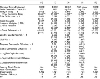
Notes: Dependent variable: Polity score normalized to run from 0 to 100. Robust t-statistics in brackets. DKSE refers to Driscoll–Kraay standard errors; RSE c/year refers to robust standard errors clustered by year; NW refers to Newey–West AR1 adjustment with one lag length; lag D.V. refers to introducing a lag of D.Polity (omitted from table). LRM standard errors estimated using the delta method: −1(b(Fiscal Reliance t − 1)/b(Polity t − 1)). Separate country and year intercepts estimated but omitted from table; F-test on joint significance of country and year dummies always highly statistically significant.
*Significant at 10%; ** 5%; *** 1%.
Our results imply that, no matter how one looks at the relationship between Fiscal Reliance and Polity, there is no evidence for a resource curse. A reader who accepts the results of the cointegration tests has to conclude that there is no resource curse, because they indicate that there is not a long-run equilibrium relationship between Fiscal Reliance and Polity. A reader who discounts the cointegration tests, and focuses on the parameter estimates from the ECM regressions, also has to conclude that there is no resource curse: the relationship between Fiscal Reliance and Polity is positive and significant, implying a resource blessing.
Panel Analysis of Total Oil Income. A skeptical reader might question these results on the grounds of sample selection bias: our Fiscal Reliance data might capture an unrepresentative sample of the world's largest resource producers. We therefore substitute Total Oil Income, which covers the entire world since 1800, as the independent variable and follow the same order of operations that we employed when we used Fiscal Reliance as the independent variable. The broad time series and cross-sectional coverage of Total Oil Income confer an additional benefit: we can split the sample in ways that allow us to search for evidence of a long-run relationship between Total Oil Income and Polity in subsets of the dataset where theory predicts a resource curse.
We split the sample by time period, threshold of resource reliance, region, per capita income when oil was first produced, and distribution of income. Regardless of how we split the sample, we find evidence suggesting that Polity and Total Oil Income are integrated of order one (results available upon request). We therefore perform the four Westerlund panel cointegration tests.Footnote 8 We often find that when we include control variables, at least of two of the four tests suggest grounds to reject the null hypothesis. In other samples, the results of the cointegration tests are less clear: sometimes only one of the tests with control variables produces a result that provides grounds to reject the null, sometimes none do; but in these cases, some of the tests that do not include control variables provide grounds to reject the null.
When we can reject the null hypothesis of no cointegration, we estimate panel ECM regressions in order to determine the sign, magnitude, and significance of the long-run relationship between Total Oil Income and Polity. When the grounds to reject the null are weaker—they suggest that there is no equilibrium relationship between oil and regime type—we nonetheless estimate ECM regressions as well. Our reasoning is as follows: in the unlikely case that either the unit root tests or the cointegration tests have yielded false negatives, it behooves us to identify and report the direction of the relationship between Total Oil Income and Polity in levels, despite the fact that there are reasons to be dubious of any inferences that can be drawn from a regression in levels between two nonstationary and noncointegrated variables (Granger and Newbold Reference Granger and Newbold1974). In short, we want to be sure that we are not overlooking any evidence that is consistent with the resource curse theory, even if there are serious grounds to doubt that evidence. We proceed subsample by subsample, first reviewing the results of the cointegration tests (Table 3, Panels A–P), and then presenting ECM regressions, focusing our discussion on the LRM.
Let us begin with the global panel of all 168 countries from 1800 to 2006 (Table 3, Panel A). When we do not include the control variables (Column 1), three of the four cointegration tests reject the null hypothesis at the 1% level, whereas the fourth test rejects the null at the 10% level. When we include conditioning variables (Column 2), two of the four tests reject the null at the 1% level.
Given that there are grounds to think that there is a long-run relationship between Total Oil Income and Polity, we want to know the direction and significance of that relationship. Table 5, Column 1, presents the results of the ECM regression with all control variables on this global panel—and the results are inconsistent with the resource curse hypothesis.Footnote 9 Instead of the negative sign on the LRM predicted by the resource curse, the LRM is positive and significant at the 1% level. We also perform the same robustness checks as we did for the Fiscal Reliance panel regressions (reported in Table 4, Columns 3, 4, and 5). Our results are always robust. We therefore do not reproduce them here (see Online Appendix 2, Data Analysis).
Error Correction Models for the Impact of Total Oil Income on Polity Score (Country Fixed Effects)

Notes: Dependent variable: Polity score normalized to run from 0 to 100. Robust t-statistics in brackets (Driscoll–Kraay standard errors estimated with Newey–West adjustment with one lag length). Obs. > avg. TOI: country–years above the Total Oil Income (TOI) mean for all country–years; obs. > avg. TOI, only oil: country–years above the TOI mean for only oil producers; obs. > 1 S.D. + avg.: country–years above one standard deviation above the mean for all country–years. LRM standard errors estimated using the delta method: −1(b(Total Oil Income t − 1)/b(Polity t − 1)). Separate country and year intercepts estimated but omitted from table; F-test on joint significance of country and year dummies always highly statistically significant.
*Significant at 10%; **5%; ***1%.
Conditional Effects. One explanation of this surprising finding is that the resource curse is perhaps a result of recent geostrategic developments. Perhaps it only exists in the post-1973 period, when dramatic increases in oil prices gave significant leverage to oil-producing countries. This allowed them to nationalize their oil industries, become price setters, and deploy the resulting windfalls to make their governments accountability-proof.
We therefore test the hypothesis that the resource curse is conditional with respect to time by truncating the dataset to 1973–2006 and then reestimate all of the models. When we do so we find that the cointegration tests suggest grounds for rejecting the null hypothesis: three of the four cointegration tests produce results that are significant at the 1% level; even when we add control variables, two of the four tests produce results that are significant at 5% or better (see Table 3, Panel C). We therefore estimate ECM models in order to determine the sign and significance of the LRM (see Table 5, Column 2)—and the results are not encouraging for the resource curse theory. Instead of the negative sign on the LRM predicted by the resource curse, the sign on the LRM is positive and highly significant.
One might argue that our regression results underestimate the negative effect of Total Oil Income on Polity because we have assumed that all increases in oil reliance are created equal. Might it be the case that an increase in Total Oil Income affects a major producer, such as Nigeria, more than it affects a minor producer, such as Belize? Or, similarly, perhaps increases in Total Oil Income only began to affect Nigeria's Polity Score negatively once it became a major producer, in the 1970s, and had no effect before that.
We therefore want to find out if there is a range of country–year observations in which increases in Total Oil Income above a critical threshold drive decreases in Polity. To do so we split the dataset into three groups—all observations above the mean of Total Oil Income of all countries, all observations above the mean of Total Oil Income for oil-producing countries only, and all observations that are at least one standard deviation above the mean of Total Oil Income for all countries. The cutoff points for these groups are $338, $971, and $2,954, respectively. We then follow the same order of operations we employed for the global panel. The cointegration tests fail to reject the null hypothesis: none of the results on the first panel approach statistical significance, only one of the tests on the second panel is significant at conventional levels, and that test only requires there to be evidence of a long-run equilibrium relationship in any single country time series (see Table 3, Panels D and E). We are unable to perform the cointegration tests on the third split sample, because there are insufficient observations at this high level of oil production. In short, the cointegration tests indicate that there is not a long-run equilibrium relationship between Total Oil Income and Polity among major oil producers.
There is always the possibility that our cointegration tests are yielding false negatives. Because it is incumbent upon us to look for evidence of a resource curse—however tenuous that evidence might be—we follow our practice of estimating ECM models when the cointegration tests fail to reject the null merely to see if the LRM has the negative sign predicted by the resource curse theory. None of the LRMs has the predicted sign (see Table 5, Columns 3, 4, and 5). In sum, neither the cointegration tests nor the ECM regressions (for those readers who are disposed to discount the cointegration tests) produce results that are consistent with the hypothesis that there is a resource curse at high levels of per capita oil production.
Perhaps it is the case that oil only has negative effects in particular geographic/cultural environments? To test this hypothesis, we group countries by region, and follow the same order of operations as above. Only the Southeast Asian panel produces results that provide grounds for rejecting the null hypothesis: when control variables are included, two of the four cointegration tests produce results that are significant at conventional levels of confidence. In the other regions, the cointegration tests fail to reject the null hypothesis: when control variables are included, none of the test statistics are significant at conventional levels of confidence for the Latin American, MENA, and Eastern Europe and Central Asia panels; and the Sub-Saharan Africa panel produces only one test statistic that is significant at conventional levels, but it is for a Group Mean Test, which only requires there to be evidence of a long-run equilibrium relationship in the series for a single country (see Table 3, Panels F, G, H, I, J). These results suggest that there likely is a long-run equilibrium relationship between Total Oil Income and Polity in Southeast Asia, but it does not identify the direction of the relationship. We therefore estimate an ECM regression, and find that the LRM has a sign opposite to that predicted by the theory of the resource curse (it is positive, though not significant—see Table 6, Column 5). Because there is always the possibility that our cointegration tests have yielded false negatives, we also estimate ECM regressions for the other regional panels to see if they produce the predicted negative signs on the LRM—and none do (see Table 6, Columns 1–4). In short, there is no evidence for a resource curse in particular world regions, regardless of whether one accepts the cointegration tests or discounts them.
Error Correction Models for the Impact of Total Oil Income on Polity Score (Country Fixed Effects)

Notes: Dependent variable: Polity score normalized to run from 0 to 100. Robust t-statistics in brackets (Driscoll–Kraay standard errors estimated with Newey–West adjustment with one lag length). MENA: Middle East and North Africa; EAST E.: Eastern Europe (see Online Appendix on Sources and Methods for the coding rules used). LRM standard errors estimated using the delta method: −1(b(Total Oil Income t − 1)/b(Polity t − 1)). Separate country & year intercepts estimated but omitted from table; F-test on joint significance of country and year dummies always highly statistically significant.
*Significant at 10%; **5%; ***1%.
Dunning (Reference Dunning2008) advances a theory about resource curses that is conditional on the distribution of income. He argues that in countries where income is unequally distributed there is a resource blessing, but in countries where income is more equally distributed there is a resource curse. To test this hypothesis, we measure income inequality using the same metric as Dunning (Reference Dunning2008)—the capital share of nonoil value added in GDP—and split the data into three groups: countries with equal distributions of income (below the mean), countries with unequal distributions of income (above the mean), and countries with very unequal distributions of income (one standard deviation above the mean).Footnote 10 For Dunning's theory to be consistent with evidence, the cointegration tests should provide grounds to reject the null; the ECM regressions on the set of equal countries should produce negative and statistically significant coefficients on the LRM; and the ECM regressions on the sets of unequal and very unequal countries should produce positive and statistically significant coefficients on the LRM.
Following our standard order of operations, we begin with the cointegration tests, which we present in Table 3, Panels K, L, and M. These suggest that there are grounds for rejecting the null hypothesis for the panels of unequal countries and very unequal countries (when control variables are included, two of the four test statistics for each panel are significant at conventional levels of confidence); but the tests fail to reject the null hypothesis in the panel of countries where income is more equally distributed (when control variables are included, none of the test statistics are significant at conventional levels). In short, the cointegration tests suggest that there may be a conditional resource blessing, but not a conditional resource curse.
Given that the results of the cointegration tests suggest that there are grounds for thinking that there is a long-run equilibrium relationship between Total Oil Income and Polity among countries with unequal income distributions, we estimate ECM regressions in order to determine the direction and statistical significance of the LRM. The results, presented in Table 7, Column 2, indicate that there is a modest resource blessing among countries with unequal distributions of income: the LRM is positive and statistically significant, but its magnitude is quite small. For every $1,000 increase in Total Oil Income per capita, Polity increases by 1.2 points (on a 0 to 100 scale). When we estimate ECM models on the subset of very unequal countries, the LRM is no longer statistically significant (results presented in Online Appendix 2, Data Analysis).
Error Correction Models for the Impact of Total Oil Income on Polity Score (Country Fixed Effects)

Notes: Dependent variable: Polity score normalized to run from 0 to 100. Robust t-statistics in brackets (Driscoll–Kraay standard errors estimated with Newey–West adjustment with one lag length). See text and Online Appendix on Sources and Methods for the coding rules behind the split-sample classifications used to group countries. LRM standard errors estimated using the delta method: −1(b(Total Oil Income t − 1)/b(Polity t − 1)). Separate country and year intercepts estimated but omitted from table; F-test on joint significance of country and year dummies always highly statistically significant.
*Significant at 10%; **5%; ***1%.
Some readers might worry that our cointegration tests on the set of equal countries are yielding false negatives. We therefore follow our practice of giving the resource curse the benefit of the doubt by estimating ECM regressions on the subset of equal countries in order to see if the LRM has the predicted negative sign. The results, presented in Table 7, Column 1, do not support the hypothesis of a conditional resource curse: the LRM has the wrong (positive) sign.
One might argue that the resource curse is conditional on the level of economic development at the time that oil is discovered: countries with high per capita incomes will be immune to the pernicious effects of petroleum, whereas countries with low per capita incomes will be cursed. To test this hypothesis, we split our dataset into three subsamples: rich countries (above the mean of GDP per capita of the set of non–oil producers when oil was first exploited in the producing country); poor countries (below the mean); and very poor countries (one standard deviation below the mean). We follow our standard order of operations, and thus begin by looking for evidence of a long-run equilibrium relationship between Total Oil Income and Polity in these three subsamples. The cointegration tests, reported in Table 3, Panels N, O, and P, fail to reject the null: when control variables are included, only one test statistic in one panel is statistically significant. Moreover, that statistic is for the Group Mean Test t (in Panel N), which only requires there to be evidence of a long-run equilibrium relationship in a single country series. In and of themselves, the cointegration tests cast doubt on the claim that poor countries are cursed by natural resources.
A skeptical reader might again worry that our cointegration tests are yielding false negatives. We therefore estimate ECM regressions in order to see whether the LRMs have the predicted negative signs. The results, reported in Table 7, are inconsistent with a conditional resource curse: the LRM for the subset of poor countries not only is positive, but is of large magnitude (Column 3). The LRM on the subsample of very poor countries also has a positive sign, and it is of even larger magnitude (Column 4). In short, a reader who discounted the cointegration tests would have to accept the fact that the LRMs indicate a resource blessing.
Regime Type as a Binary Variable. Some researchers claim that regime type is inherently dichotomous (Przeworski et al. Reference Przeworski, Alvarez, Cheibub and Limongi2000). We therefore estimate a series of dynamic, conditional fixed effects logit regressions with Regime as the dependent variable. This estimation technique allows us to calculate separate estimates for those countries observed as democratic and those observed as autocratic—and then see whether they switch regime type as a result of increased resource reliance. This estimation strategy also allows us to continue to control for time-invariant heterogeneity between countries. Although we report the results of these regressions in a separate online supplement (Online Appendix 3, Conditional Logit Regressions, at www.journals.cambridge.org/psr2011001), we summarize them here. Democracies are less likely to break down as Total Oil Income increases; autocracies are more likely to transition to democracy as Total Oil Income increases. In short, when we substitute a binary measure of democracy for Polity, the evidence does not support the hypothesis of a resource curse but instead provides some evidence of a resource blessing.
Difference in Differences. By focusing on variance over time within countries, we have addressed the problem of time-invariant omitted-variable bias. To put it concretely, we are implicitly comparing Venezuela to itself over time in order to see whether increases in its resource reliance explain lower levels of Polity, controlling for the effects of higher GDP per capita and possible democratic contagion effects from other countries. One might argue, however, that Venezuela might have democratized even faster, or more fully, had it not developed an oil-based economy. The key to addressing this issue is the specification of a more exacting counterfactual than the before-and-after comparison implied by our ECM regressions. Producing such a counterfactual requires us to ask a question of the following type: what would Venezuela's Polity have been today had it not been earning oil rents since 1917?
This counterfactual Venezuela does not, of course, exist; but we can observe the political trajectory of a set of countries that were broadly similar to Venezuela, in terms of history, geography, culture, level of economic development, and degree of democratization before Venezuela became increasingly reliant on oil, but that did not subsequently become major oil producers. That set of countries is the other nations of Latin America that did not become resource-reliant. We therefore return to using Polity as the dependent variable but now transform it: we net out the difference in Polity between oil-producing countries and a synthetic, non–resource reliant country that is represented by the average polity score of the non–resource reliant countries in the oil-producing country's geographic/cultural region (our procedure for identifying the non–resource reliant countries can be found in Online Appendix 1, Sources and Methods). We refer to this variable as Net Polity. This transformation allows us to see if the yearly differences in the changes in Polity between treatment and control groups are a function of changes in the dose of oil, after controlling for the same set of covariates as in the previous regressions. Because we can reject the null of nonstationarity for Net Polity across the models that follow, we no longer have to worry about cointegration (results available upon request).
Our approach is therefore a refinement of a typical difference-in-differences model that captures the treatment effect with a dummy variable. We run an OLS model with the following functional form:

where Y is an (n × 1) vector of observations on the dependent variable, Δ is the first-difference operator, X is an (n × k) matrix of n observations on k explanatory variables, β is a (k × 1) vector of parameters, n is a country fixed effect potentially correlated with variables in X, v is a year fixed effect potentially correlated with variables in X, and u is an (n × 1) vector of disturbance terms that are possibly heteroskedastic and correlated within countries. Both n and v imply that a dummy variable for each country in the dataset (except for one) is included in the equation and a year dummy for each year in the panel dataset (except for one) is also included. Heterogeneous intercepts are estimated by country and year (the φ and λ vectors, respectively). We employ the same control variables as our earlier regressions, and estimate Driscoll-Kraay standard errors with a Newey-West adjustment with one lag length.Footnote 11
We present the results in Model 1 of Table 8. The Total Oil Income coefficient is negative, but far from statistically significant. One might argue that the reason for lack of significance is endogeneity: for example, perhaps countries that are transitioning toward democracy pump more oil than they did under autocracy because the new regime needs to placate voters’ demands for public goods.
Panel Fixed Effects Estimation, Difference-in-differences Models for the Impact of Total Oil Income on Net Polity

Notes: Net Polity calculated from Polity scores normalized to run from 0 to 100. Robust t-statistics (calculated with Driscoll–Kraay standard errors) in brackets. See text and Online Appendix on Sources and Methods for Net Polity coding; static models run with Newey–West AR1 adjustment with one lag length. A battery of heteroskedasticity tests reject the hypothesis that the error term is homoskedastic; Arellano Bond serial corellation test fail to reject AR(1); thus, IV GMM (instrumental variables generalized method of moments) approach is taken (only second-stage output shown) with D.Total Oil Income as potentially endogenous, instrumented with Proven Oil Reserves, Oil Reserves per Surface Area, and Total Regional Oil Reserves (all in levels), and with weighting matrix estimated by an Eicker–Huber–White robust covariance estimator. Results are robust to introducing Total World Oil Reserves as an additional instrument; results are also robust to excluding any of the other instruments (each enters significantly as a determinant of D.Total Oil Income in first-stage regression). ARDL refers to Autoregressive Distributed Lag Model; standard errors for the Total Change made by Total Oil Income estimated using the delta method: ((ΔTotal Oil Income t + ΔTotal Oil Income t − 1)/(1−(ΔPolity t − 1)). Separate country and year intercepts estimated but omitted from table.
*Significant at 10%; **5%; ***1%.
We therefore adopt an instrumental-variables approach to evaluate this hypothesis before we continue with the difference-in-differences framework. We construct a dataset on proven oil reserves for virtually every oil producer in the world on an annual basis from 1943 to 2006, and use it to generate three instruments in levels: Reserves, Reserves per Surface Area, and Total Reserves in the Region (see Online Appendix 1, Sources and Methods). We then estimate a GMM two-stage instrumental-variables regression with country and year fixed effects.Footnote 12 We treat Total Oil Income in first differences as potentially endogenous, and therefore instrument it with Reserves, Reserves per Surface Area, and Total Reserves in the Region. All three instruments enter the first stage of the regression as independently and jointly significant determinants of Total Oil Income (in first differences). This stage also includes all of the control variables employed previously (results not reported because of space constraints). The independent variable of interest in the second stage (Model 2 of Table 8) is the predicted values of Total Oil Income (in first differences) from the first-stage regression. The dependent variable is Net Polity (in first differences). The instruments are valid according to a Hansen J-test of the overidentifying restrictions (see bottom of Model 2), which means that we cannot reject the null hypothesis that the instruments are exogenous.
Table 8, Model 2 suggests that changes in Total Oil Income are not endogenous to changes in Net Polity: the difference in the Sargan C-test strongly indicates that we cannot reject the null that Total Oil Income is exogenous (see bottom rows of Model 2). Therefore, although the sign on Total Oil Income (in differences) in the second stage of the regression is negative and significant at the 10% level, there is no justification for using instrumental variables. In fact, if we drop the instrumental-variable approach, and run a regular, static OLS regression on the same subsample as for Model 2, we obtain a result that is nowhere near statistically significant (see Online Appendix 2, Data Analysis). In addition, if we employ the instrumental-variables approach on subsamples that are truncated with respect to time, we again cannot reject the null that Total Oil Income is exogenous. Moreover, in these specifications, the second stage of the regression now produces coefficients on Total Oil Income that are either far from statistically significant or have the wrong (positive) sign (see Online Appendix 2).
Perhaps the results discussed above, which are not consistent with the hypothesis of a resource curse, are a function of the fact that our models only capture the instantaneous impact of changes in Total Oil Income on changes in Net Polity? What if the changes in Net Polity induced by changes in Total Oil Income are spread out over a period of several years? We therefore estimate a rational, infinitely distributed lag model as an autoregressive distributed lag model (ARDL) in first differences following Wooldridge (Reference Wooldridge2006, 638) in order to calculate the total change in Net Polity made by a change in Total Oil Income. Specifically, X in equation (3) now includes the one-year lag of the (differenced) dependent variable and a lag of (differenced) Total Oil Income to calculate the total change made by Total Oil Income on Net Polity, with the standard errors of this coefficient computed via the delta method.
Table 8, Model 3 presents the results of the full panel, and it provides no evidence in favor of a resource curse. The coefficient on the immediate impact of Total Oil Income continues to be negative, but far from significant. The total change distributed over all periods, however, is positive and statistically significant at the 1% level. We then search for possible conditional effects under which changes in Total Oil Income effect changes in Net Polity by employing the same split-sample techniques that we used in the panel ECM approach: we estimate all regressions on subsamples of the dataset split by time period, oil income thresholds, region, income distribution, and economic development.
None of these regressions produce results that are consistent with the resource curse, which is to say a statistically significant negative coefficient on the Total Change Made by the Change in Total Oil Income. Table 8, Models 4–7, presents only those results in which the coefficient on the Total Change Made by Total Oil Income is significant at 5% or better (the rest of the results are available in Online Appendix 2, as are results for static models). Of the 15 conditional-effects regressions that we estimate, only one (Sub-Saharan Africa) produces the predicted negative coefficient—and that result is far from statistically significant. Fourteen of the 15 regressions produce coefficients with the wrong (positive) sign, and of these 7 are statistically significant at the 1% level, whereas an additional 2 are significant at 10%. To the degree that any of the regressions produce a statistically significant, negative coefficient on the Immediate Impact of Changes in Total Oil Income (Total Oil Income in t), only two reach the 10% level. Moreover, these two negative coefficients are eclipsed by positive coefficients of greater magnitude on the lagged value of Changes in Total Oil Income that are statistically significant at the 1% level. In short, the regressions rule out even a short-run resource curse.
With so many positive and statistically significant coefficients on the Total Change Made by Total Oil Income, one may wonder if there is a resource blessing. The answer depends on how one weighs the statistical significance of coefficients versus their magnitude. An emphasis on statistical significance would indeed suggest a resource blessing. The small magnitude of the positive coefficients, however, would suggest that if there is a resource blessing, its effect is minimal.
Robustness Tests: Total Fuel Income and Total Income from Fuel and Metals. One might argue that our measure of resource reliance, Total Oil Income, leaves out the rents generated by the production of other fuels and minerals, and that if we accounted for the income from those additional sources we would find evidence for a resource curse. We therefore reestimate all of the difference-in-differences regressions presented above, but substitute Total Fuel Income (oil, natural gas, and coal) and Total Resource Income (oil, natural gas, coal, precious metals, and industrial metals) for Total Oil Income. The results do not overturn our regressions on Total Oil Income, and thus we do not report them here (they are available in Online Appendix 2). The sign of the coefficients of interest remain positive. The one difference that we pick up is that the coefficients of interest are somewhat less statistically significant—though they still achieve significance of 10% or better.
CONCLUSION
We have developed metrics that allow us to analyze the longitudinal relationship between countries’ resource dependence and their regime type. We observe countries prior to their becoming resource-reliant, and evaluate whether increases in resource rents affected their political development—both relative to themselves before resource dependence and relative to the experience of countries that were similar to them, save for resource dependence. Our results indicate that oil and mineral reliance does not promote dictatorship over the long run. If anything, the opposite is true. These results hold even when we search for a host of conditional effects suggested by the literature. This is not to say that there may not be specific instances in which resource rents might have helped to sustain a dictatorship. It is to say, however, that there is a big difference between pointing to these instances and making sweeping, lawlike statements.
The implications of our analysis extend beyond the literature on the resource curse. Researchers in comparative politics are keenly interested in explaining processes that occur within countries over time, such as industrialization, the rise of the welfare state, the centralization of taxation, transitions to democracy, and civil conflict. In studying these processes, however, comparativists often rely on datasets with a limited time dimension and employ pooled regression techniques that treat countries as homogenous units. These methods increase the risk that correlation will be mistaken for causation. A time series approach to data transcends concerns about bias. When a hypothesis is not about static differences between countries, but about complex changes that take place within countries over time, long-run historical datasets provide a better fit between theory and evidence. This approach not only allows researchers to model dynamics, but also is conducive to the specification of counterfactuals—both of which allow researchers to improve causal inference.
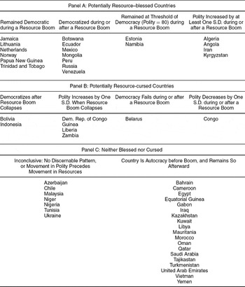
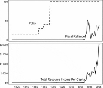
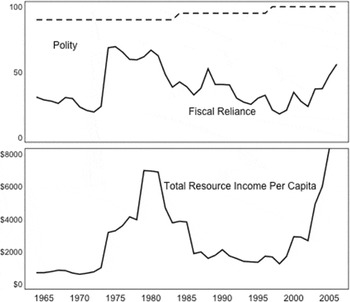
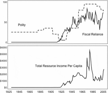
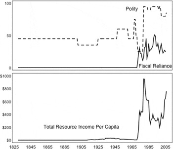
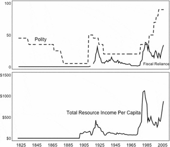
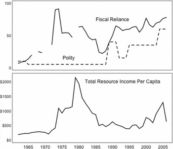
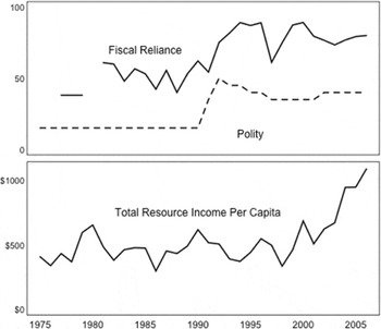
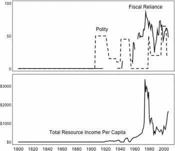
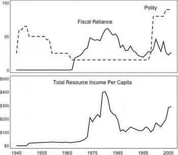
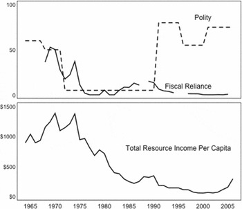
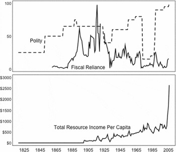
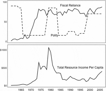
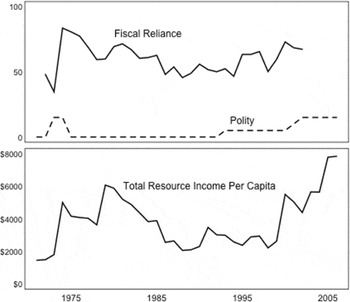
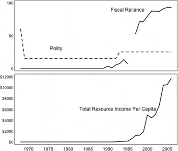
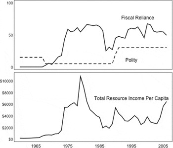
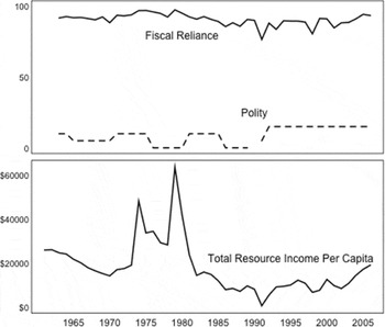
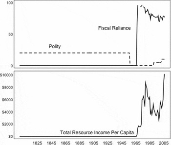
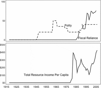
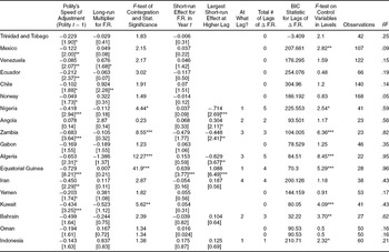
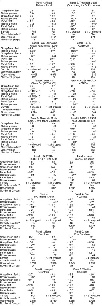
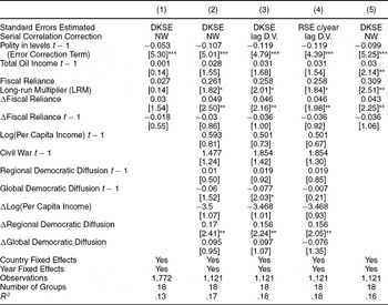
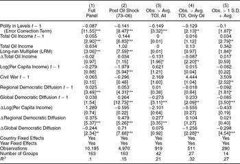
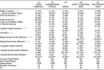
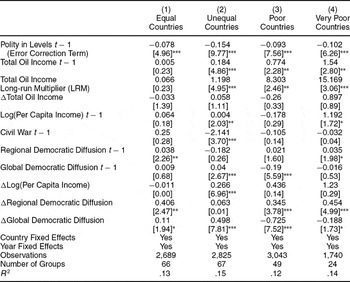
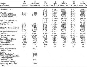




Comments
No Comments have been published for this article.