

1 Introduction
1.1 Phonetic interpolation as evidence for phonological underspecification
Early generative phonology assumed that every segment is specified for every distinctive feature and receives ‘a phonetic command’ for all the phonetic dimensions represented by distinctive features (e.g. Chomsky & Halle Reference Chomsky and Halle1968: 403–419). However, this assumption has given way to various proposals regarding underspecification (Archangeli Reference Archangeli1988, Keating Reference Keating1988). Building on the phonological theory of feature underspecification, Keating (Reference Keating1988) observed that some segments lack a particular ‘phonetic target’ in some dimension. One example is English /h/, which on spectrograms can look like an interpolation from the preceding segment to the following segment. Another example is nasal airflow data in English (Cohn Reference Cohn1993), in which vowel nasalisation before a tautosyllabic nasal consonant involves phonetic interpolation from [―nasal] to [+nasal], with the vowel itself being unspecified for [nasal]. Other research has argued that various types of vocalic transitions between consonants are not phonologically specified, but, rather, are best described as periods of open vocal tract with no vocalic target. Cases such as this include the transitional vocoids surfacing between consonants in Yine/Piro (Hanson Reference Hanson2010: 28), the vocoid that surfaces between final consonant clusters in Moroccan Arabic (Gafos Reference Gafos2002) and the production of phonotactically illicit consonant clusters by non-native speakers (Davidson Reference Davidson2010). See Hall (Reference Hall2006: 390) for a list of 29 languages with phonologically inert ‘excrescent vowels’ and a discussion of their common properties.
Intonation is another area in which the idea of phonetic underspecification has played a central role in theory development. Pierrehumbert (Reference Pierrehumbert1980) argues that modelling intonational contours of English can be best achieved by only sparsely specifying high and low targets, rather than specifying all syllables for tone. Pierrehumbert & Beckman (Reference Pierrehumbert and Beckman1988) demonstrate that the apparent H-tone spreading in Japanese unaccented words proposed by Haraguchi (Reference Haraguchi1977) is better characterised with phonetic underspecification. The phonetic data shows a roughly linear decline from a H tone to the next L tone (see also the discussion in §6.4). Building on these observations, sparse tonal specification has been extended to the intonational analysis of many languages (e.g. Pierrehumbert & Beckman Reference Pierrehumbert and Beckman1988, Myers Reference Myers1998), and now constitutes a fundamental assumption in the autosegmental metrical theory of intonation (Arvaniti & Ladd Reference Arvaniti and Ladd2015, Jun Reference Jun2014; cf. Xu et al. Reference Xu, Lee, Prom-on and Liu2015).
Generalising across these cases, there is a large body of literature arguing that phonetic behaviour is determined by sparse (surface) phonological specification. Determining which phonetic dimensions are under phonological control on the basis of the phonetic signal alone is challenging, as it involves discovering phonological control in the presence of many other factors that influence the data. At times, the indeterminacy of phonetic data has given rise to highly disparate characterisations of the same language by different researchers. For example, Tashlhyit Berber has been described both as a language with many epenthetic vowels (Coleman Reference Coleman2001) and as one which has syllabic consonants and no epenthetic vowels (Dell & Elmedlaoui Reference Dell and Elmedlaoui1985, Ridouane Reference Ridouane2008). This dichotomy hinges on whether transitions between consonants are treated as being under the phonological control of vowels or not, and has been largely resolved through converging evidence from multiple data sources, including appropriate phonetic analyses (Ridouane Reference Ridouane2008). Similar ambiguity is present in other languages. Hall (Reference Hall2006) argues that vocoids between stops and sonorants in Hocank (Winnebago), which are invisible for the purpose of primary stress placement, are not true vowels, but merely open transitions between consonants. Other researchers have argued on theoretical grounds that the Hocank vocoids are epenthetic vowels (Davis & Baertsch Reference Davis, Baertsch, Cairns and Raimy2011), which makes stress-placement rules opaque and has consequently spawned a range of theoretical proposals to account for stress–epenthesis interactions, including iterative application of metrical feet (Hale & Eagle Reference Hale and Eagle1980), positional faithfulness (Alderete Reference Alderete, Beckman, Dickey and Urbanczyk1995) and ordered application of the same epenthesis process in different environments (Strycharczuk Reference Strycharczuk2009). In the absence of a robust phonetic record, other researchers have reinterpreted the facts, arguing that stress occurs on the epenthetic vowel (Stanton & Zukoff Reference Stanton and Zukoff2018). In other languages, vowels that are invisible to stress have been shown to differ variably in phonetic quality and duration from vowels that influence stress placement, raising questions about the degree of surface opacity (Hall Reference Hall2013). The broader point is that theoretical debates can emerge from ambiguity about surface phonological form, particularly when appropriate analyses of phonetic data are unavailable. This paper develops analytical tools to strengthen the interpretation of surface phonological (non-)specification on the basis of phonetic data.
In many of the phonological domains described above, phonetic interpolation has been a key argument for the phonological non-specification of some dimension, whether it be tone, a phonological feature or a segment. The general logic is as follows. Consider an ABC sequence, where the phonological specification of B is at issue and B is assumed to control a phonetic parameter p. Whether observed in the domain of intonation (Pierrehumbert & Beckman Reference Pierrehumbert and Beckman1988: 37–38), vowels (Browman & Goldstein Reference Browman, Goldstein, Docherty and Ladd1992) or consonants (Cohn Reference Cohn1993, Keating Reference Keating1988), phonetic interpolation on dimension p between A and C has been motivated as an argument for the ‘targetlessness’ of B.
Rigorously assessing phonetic interpolation is not always straightforward, owing in part to the natural variability associated with phonetic data. Moreover, listeners show remarkable tolerance for phonetic variation (Shaw et al. Reference Shaw, Best, Docherty, Evans, Foulkes, Hay and Mulak2018). Importantly, the specific patterning of phonetic variability can reveal the phonological form that structures the signal (e.g. Shaw et al. Reference Shaw, Gafos, Hoole and Zeroual2011). Explicitly modelling how different phonological forms structure natural variation in the phonetic signal provides a way to assess the likelihood that observed phonetic data can be attributed to the presence of a phonologically specified target or, alternatively, to the absence of such specification. Returning to the case of ABC, appropriately leveraging phonetic data to assess phonological specification of B based on some phonetic parameter p requires distinguishing complete targetlessness from phonetic reduction due to, for example, susceptibility to coarticulation with surrounding segments (cf. Recasens & Espinosa Reference Recasens and Espinosa2009) or high predictability in context (e.g. Cohen Priva Reference Cohen Priva2017, Shaw & Kawahara Reference Shaw and Kawahara2017). Although rigorous assessment of phonetic interpolation is a challenging problem, it is one that can greatly enhance our confidence in the identity of surface phonological representations.
This paper develops a general methodology for assessing feature specification in surface phonological representations on the basis of the phonetic signal. A key tenet of our approach is to express abstract phonological hypotheses in the units of the phonetic data. Like snowflakes and fingerprints, no two phonetic signals are identical, even those that actuate identical phonological structures. This fact dictates that rigorous assessment of phonological hypotheses on the basis of phonetic data requires a probabilistic model of how phonological form maps to the phonetic signal. Following recent approaches to syllable micro-prosody (Gafos et al. Reference Gafos, Charlow, Shaw and Hoole2014, Shaw & Gafos Reference Shaw and Gafos2015), we seek to estimate distributions that relate low-dimensional phonological hypotheses to high-dimensional phonetic data. Accordingly, we construct stochastic phonetic models that are parameterised by our phonological hypothesis as well as by the level of variability naturally present in the phonetic data.
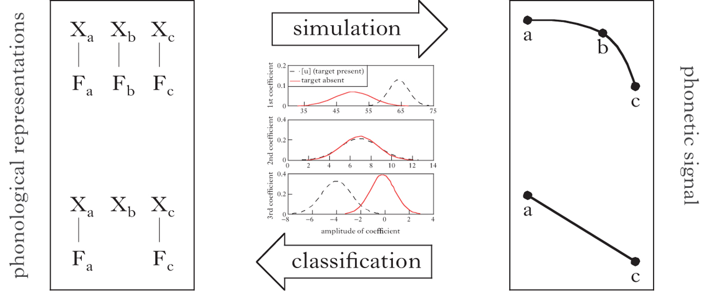
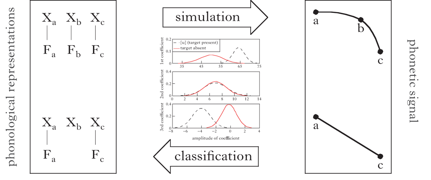
A schematic of the approach is presented in Fig. 1. The key idea is to link surface phonological form (left) to time-varying phonetic data (right), through the stochastic processes of simulation and classification (middle). Our proposal for the stochastic representational space that supports these processes makes use of parametric (Gaussian) distributions over frequency components of the phonetic signal. We use Discrete Cosine Transform (DCT) to decompose high-dimensional phonetic data into a low-dimensional frequency space that can be mapped to phonological form. In this frequency space, we formulate competing phonological hypotheses, including the phonetic interpolation (‘targetless’) hypothesis (bottom of Fig. 1). For the purposes of this paper, we follow others (e.g. Lammert et al. Reference Lammert, Goldstein, Ramanarayanan and Narayanan2014) in making the simplifying assumption that interpolation will take the form of a linear transition between flanking segments, though we return to this assumption in §6.3.Footnote 1 We estimate distributions over signal components in frequency space, and sample from these distributions to convert competing phonological hypotheses into the real-world spatial-temporal dimensions of the data. This step, simulation, factors into the analysis the range of natural variability found in the phonetic data, allowing us to generate realistically variable phonetic signals from discrete phonological hypotheses. Finally, we train a Bayesian classifier on the data simulated from competing phonological hypotheses (full lingual target vs. no lingual target), and use it to compute, on a token-by-token basis, the probability of interpolation (no lingual target), given the phonetic signal. Taken together, this computational toolkit yields stochastic representations that support rigorous assessment of ‘targetlessness’ through simulation and classification of phonetic data.
Schematic depiction of the modelling approach. The left box shows phonological representations with (top) and without (bottom) a particular feature, Fb, while the right box shows corresponding phonetic signals with (top) and without (bottom) a phonetic target for Fb. The link between phonological form and the phonetic signal is a stochastic representational space - Gaussian distributions over (DCT) frequency modulation components - used for simulation and classification.
1.2 Japanese high vowel devoicing
To illustrate our computational approach, we examine high vowel devoicing in Tokyo Japanese (Tsuchida 1997, Kondo Reference Kondo, van de Weijer, Nanjo and Nishihara2005, Fujimoto Reference Fujimoto and Kubozono2015). A key debate regarding this phenomenon is whether the surface phonological representation contains a vowel or not. A classic description of the facts is that high vowels are devoiced between two voiceless consonants, and after a voiceless consonant before a pause. As we will see below, one proposal is that the vowel is not only devoiced, but entirely absent from the surface representation, due to deletion. When vowels are devoiced, it is difficult to ascertain from the acoustics whether they are also deleted. For this reason, we look to the articulatory signal to adjudicate between competing proposals, taking the presence or absence of a lingual articulatory target for the vowel as an indicator of surface phonological specification. We consider four hypotheses, stated in (1).
(1)

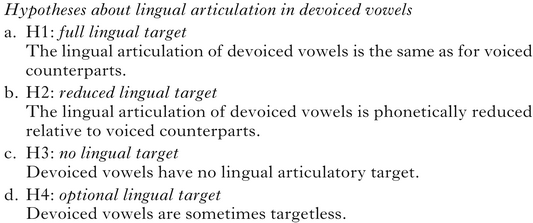
Several previous studies relate to one or more of these hypotheses. Kawakami (Reference Kawakami1977: 24–26) argues that vowels delete in some phonological environments (as in H3) and devoice in others. Sometimes, the only trace of a vowel found in the (acoustic) phonetic signal is vowel-conditioned allophony on surrounding consonants, which has led some researchers to conclude that the vowel is entirely deleted (Beckman Reference Beckman1982, Beckman & Shoji Reference Beckman and Shoji1984). If deletion is phonological, as argued by Kondo (Reference Kondo, Nakayama and Quinn2000), then the vowel should not exhibit a lingual gesture, predicting H3. Devoicing in consecutive syllables is often prohibited, and Kondo suggests that this prohibition stems from a constraint against complex onsets or codas. Even if vowel devoicing is due to phonological deletion, some studies show that its application is optional or variable (Fujimoto Reference Fujimoto and Kubozono2015, Nielsen Reference Nielsen2015), suggesting H4.
On the other hand, Tsuchida (1997) and Kawahara (Reference Kawahara2015) argue that bimoraic foot-based truncation, as discussed by Poser (Reference Poser1990), counts a voiceless vowel as one mora (e.g. [su̥to] in [su̥toraiki] ‘strike’). If [u] was completely deleted, losing its mora, the bimoraic truncation should result in *[stora], but in fact devoiced vowels always count toward the bimoraic requirement. This sort of proposal implies that the lingual gesture of devoiced high vowels should be phonologically present, and predicts either H1 or H2. In particular, H1 is predicted by a ‘gestural overlap theory’ of high vowel devoicing (Jun & Beckman Reference Jun and Beckman1993, Beckman Reference Beckman, Otake and Cutler1996, Jun et al. Reference Jun, Beckman and Lee1998). In this theory, high vowel devoicing occurs when laryngeal abduction gestures of surrounding consonants heavily overlap with the vowel. In this sense, high vowel devoicing processes in Japanese (and Korean) are ‘not … phonological rules, but … the result of extreme overlap and hiding of the vowel's glottal gesture by the consonant's gesture’ (Jun & Beckman Reference Jun and Beckman1993: 4). This passive devoicing hypothesis would predict that lingual gestures remain intact (H1). Even if devoiced high vowels are not phonologically deleted or otherwise targetless, it would not be too surprising if the lingual gestures of high vowels were reduced. Due to devoicing, the acoustic consequences of a reduced lingual gesture would not be particularly audible. Hence, from the standpoint of an effort–distinctiveness trade-off, we expect reduction of oral gestures in high devoiced vowels (H2).
We use the general methodology described in §1.1 to distinguish between the hypotheses in (1) on the basis of phonetic data. In particular, distinguishing between H2 and H3 is a specific case of the general issue raised in §1.1. How do we know that a phonetic signal lacks a phonological target (H3), rather than being reduced (H2)? Although the empirical material used to demonstrate our approach comes from Japanese high vowel devoicing, the question that we are addressing is more general: how do we assess the role of phonetic interpolation in confirming or rejecting phonological specification? Some potential broader applications of our proposed toolkit are discussed in §6.4.
The remainder of the paper is organised as follows. §2 describes the experimental methods involved in collecting articulatory data. §3 and §4 motivate the computational approach, specifically the tools used for simulation (§3) and classification (§4). §5 provides an analysis of the data addressing the hypotheses in (1). §6 provides some discussion of the results, as well as alternative approaches to assessing surface phonological specification on the basis of phonetic data.
2 The electromagnetic articulography experiment
The phonetic data used to illustrate our computational approach were drawn from a larger experiment using electromagnetic articulography (EMA) to track the movement of fleshpoints on the tongue during the production of voiced and voiceless vowels in Tokyo Japanese. The full report of the experiment can be found in Shaw & Kawahara (Reference Shaw and Kawahara2018b). This paper focuses on illustrating the computational tools.
2.1 Speakers
Six native speakers of Tokyo Japanese (three female and three male) participated. They were aged between 19 and 22 at the time of the study. They were all born in Tokyo and had spent no more than three months outside the Tokyo region.
2.2 Materials
The stimuli in the experiment consisted of words presented in the carrier phrase /ookee _ to itte/ ‘Ok, say _’. /ookee/ was selected because it ends in /e/, so that the tongue would be in a non-high position at the start of the target word. A rise in tongue position from /e/ to /u/ would suggest the presence of a vowel target for /u/. To illustrate the computational approach, we focus on the two dyads (i.e. four words) in (2), which form a subset of the stimulus items in the experiment reported in Shaw & Kawahara (Reference Shaw and Kawahara2018b).
(2)

In these words, the target vowel /u/ occurs in either a devoicing environment (a) or a voiced environment (b). In both contexts, /u/ is unaccented. These words were randomised in a list of 16 other words, ten of which did not contain high vowels in a devoicing context. All words were randomly displayed within the carrier phrase, in normal Japanese script. Participants were instructed to speak as if they were making a request of a friend. Each participant produced a total of 10–15 repetitions of each target word.
2.3 Equipment
We used an NDI Wave EMA system sampling at 100 Hz to capture articulatory movement in 3D. The spatial accuracy of this system is generally within 0.5 mm. NDI Wave 5DoF sensors were attached to three locations on the sagittal midline of the tongue, and on the lips, jaw (below the lower incisor), nasion and left/right mastoids. The height of the tongue-dorsum (TD) sensor is the focus of our analysis (lip data is reported in Appendix B).Footnote 2 The TD sensor was the most posterior of the three sensors on the tongue, attached as far back as was comfortable for the participant (~5–6 cm behind the tip). Acoustic data were recorded simultaneously at 22 KHz with a Schoeps MK 41S supercardioid microphone.
2.4 Post-processing
We recorded the bite plane of each participant by having them hold a rigid object between their teeth, with three 5DoF sensors attached to it. Head movements were corrected computationally after data collection with reference to three sensors on the head, the left/right mastoid and nasion sensors, and the three sensors on the bite plane. The head-corrected data was rotated so that the origin of the spatial coordinates corresponded to the occlusal plane at the front teeth.
2.5 Trajectories for analysis
We first visualised the data using the Matlab-based software Mview (Tiede Reference Tiede2005), which displays the EMA movement trajectories along with the waveform and spectrogram from the audio signal. In Mview, we verified that /u/ was devoiced in devoicing environments by visual inspection of the spectrogram. At this stage of analysis, we also identified articulatory landmarks associated with V1 and V3, the vowels preceding and following the target /u/. The point of minimal velocity in the TD signal corresponding to the location of V1 and V3 in the spectrogram, a reliable method of parsing vowel targets in articulatory data (for discussion, see Blackwood Ximenes et al. Reference Blackwood Ximenes, Shaw and Carignan2017), was used to left-delimit (V1) and right-delimit (V3) the interval containing /u/, i.e. /V1CuCV3/. This interval was the subject of all subsequent analyses. To illustrate the raw data, at times we also provide plots of longer intervals, so that movements of following consonants can also be visualised.
2.6 Preview of raw data
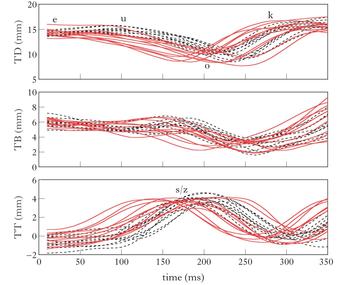
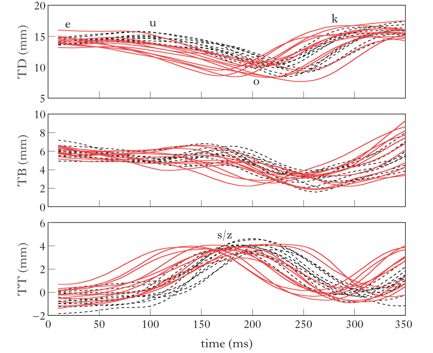
A full analysis of the data is provided in §5. Here we preview the raw data, in order to illustrate the general difficulty involved in assessing phonological specification from continuous phonetic data. Figure 2 provides representative data from one speaker, S1, producing eleven repetitions of the minimal pair /ɸusoku/ ~ /ɸuzoku/. The movement trajectories span a window from the end of /ee/ in /ookee/ to the /k/ in /ɸusoku/ or /ɸuzoku/. In line with descriptions of high vowel devoicing in contemporary Tokyo Japanese, this speaker produced voiced /u/ in /ɸuzoku/ and always devoiced /u/ in /ɸusoku/ (Shaw & Kawahara Reference Shaw and Kawahara2018b). Of interest for our case study is whether the lingual gesture of the devoiced vowel in /ɸusoku/ has an articulatory target. The top panel of Fig. 2 shows the height of the TD sensor (y-axis) over time (x-axis) with /ɸusoku/ (devoiced /u/; solid line) and /ɸuzoku/ (voiced /u/; dashed line). The middle and bottom panels shows movement of the tongue blade (TB) and tongue tip (TT). For the portion of the figure corresponding to /u/, the TD is lower for devoiced /u/ than for voiced /u/. At the very least, this pattern indicates that the devoiced vowel is phonetically reduced in this subset of the data. In the remainder of this paper, we describe a computational approach to evaluating the four hypotheses in (1) on the basis of continuous phonetic data, such as that shown in Fig. 2.
Lingual articulatory trajectories for a female speaker of Tokyo Japanese, S1, producing /ɸusoku/ (solid lines) and /ɸuzoku/ (dashed lines). The y-axis shows the height of the sensors. The trajectories span a 340 ms window starting from the /e/ of the carrier phrase and extending to the TD rise for the /k/ near the end of the words. Subsequent analysis focuses just on the interval from /e/ to /o/.
3 Simulation
This section introduces the computational tools that are used to simulate competing phonological hypotheses in the dimensions of the data. We estimate distributions over a small number of parameters that characterise the phonetic data, so that we can simulate realistically variable trajectories actuating phonological hypotheses, including the no lingual target hypothesis (H3).
As a starting point, we assume that the articulators follow direct paths between articulatory goals (cf. Keating Reference Keating1988, Browman & Goldstein Reference Browman, Goldstein, Docherty and Ladd1992). The idealised movement trajectory corresponding to the no lingual target hypothesis would therefore be a linear trajectory from V1 to V3 (Browman & Goldstein Reference Browman, Goldstein, Docherty and Ladd1992, Choi Reference Choi1995, Lammert et al. Reference Lammert, Goldstein, Ramanarayanan and Narayanan2014). In real articulatory data, fleshpoint trajectories are never straight lines. There are well-studied cases in which tongue trajectories are curved because of biomechanical factors even when the idealised movement based on phonological form would dictate a linear trajectory (Mooshammer et al. Reference Mooshammer, Hoole and Kühnert1995, Perrier et al. Reference Perrier, Payan, Zandipour and Perkell2003). To account for the numerous perturbations, biomechanical and otherwise, of linear trajectories between articulatory goals in speech production, we take a stochastic, data-driven approach, modelling actual trajectories as noisy actuations of phonological goals (Shaw et al. Reference Shaw, Gafos, Hoole and Zeroual2009, Shaw & Gafos Reference Shaw and Gafos2010, Shaw & Davidson Reference Shaw and Davidson2011).
Consider again Fig. 2. Since we are interested in the presence of a vowel, we focus on TD movement, which is the primary articulator for (non-front) vowels (see e.g. Wood Reference Wood1979). The trajectories begin with the vowel /e/ of the carrier phrase preceding the target words /ɸusoku/ and /ɸuzoku/. The TD starts out high for the vowel /e/. The vowel /u/, if it is present, would follow the /e/. Some tokens show a slight rise in TD height at the start of the trajectory, which is expected if the TD rises in height from /e/ to /u/; many tokens, however, particularly those of /ɸusoku/, show a monotonic decrease in height from /e/ to /o/, which is expected if there is no lingual target for /u/. The modelling addresses whether the observed trajectory from /e/ to /o/ is different from a realistically variable linear trajectory between /e/ and /o/. If so, this would support the phonetic reduction hypothesis (H2); if not, the result would support the no lingual target hypothesis (H3), at least for some tokens (H4).
3.1 Discrete Cosine Transform
Due to the 100 Hz sampling rate used in the EMA recording, there is one data point for every 10 ms, e.g. the 340 ms TD trajectories in Fig. 2 consist of 35 data points per trajectory. The data points in a trajectory are not statistically independent. Rather, the height of the TD at any point in time, τ, is closely related to the height of the TD at earlier (τ−1) or later (τ + 1) time points. At a deeper level, the statistical dependencies between data points across the entire trajectory are due (at least in part) to phonologically controlled movement. We use Discrete Cosine Transform (DCT), the first computational tool in our toolkit, to capture dependencies between data points. Doing so allows data compression and sparse representation, which both simplifies subsequent computation and facilitates generalisation to new data.
DCT represents the data as sums of cosines of different frequencies and amplitudes. In expressing spatial data in terms of harmonic components (i.e. frequency space), DCT is similar to Fast Fourier Transform, which is typically used to construct spectrograms from the acoustic signal. The main advantage of DCT, in particular for our purpose, is that it represents the data with a small set of parameters, a general property of DCT (Jain Reference Jain1989: 151). In addition, as we will see below, each of the DCT coefficients may have a clear linguistic interpretation. It is also important that DCT has a known inverse function, which we use to simulate TD trajectories from DCT components. Each cosine component of a DCT has an amplitude coefficient that is fitted to the data. We interpret the amplitude of the cosines as the degree to which a corresponding gesture modulates the TD trajectory. DCT has been used in some previous phonetic studies, which have shown that phonetic signals, particularly changes in vowel formants over time, can be represented quite well with a small number of cosine components (Watson & Harrington Reference Watson and Harrington1999, Elvin et al. Reference Elvin, Williams and Escudero2016).
A mathematical expression of DCT transform is provided in (4). In the numerical expression, y(k) is the amplitude of the kth cosine component. This is the output of the DCT. The other terms in the equation are as follows: L is the length of the trajectory (i.e. the number of data points); x(n) is the trajectory of the data being modelled; w(k) is a constant determined by the values of k and L: w(k) = (1/√L) when k = 1 and w(k) = √(2/L) otherwise. The first DCT coefficient, y(1), defines a straight line at a position above the average value of the data. This is because when k = 1, the term of the cosine function is zero. This means that the first coefficient is equal to (3), the sum of all data points in the trajectory divided by the square root of the number of data points.
(3)

Each subsequent DCT component defines a cosine of increasing frequency, as increases to k linearly increase the term of the cosine function.
(4)
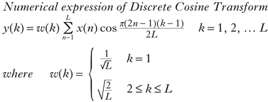
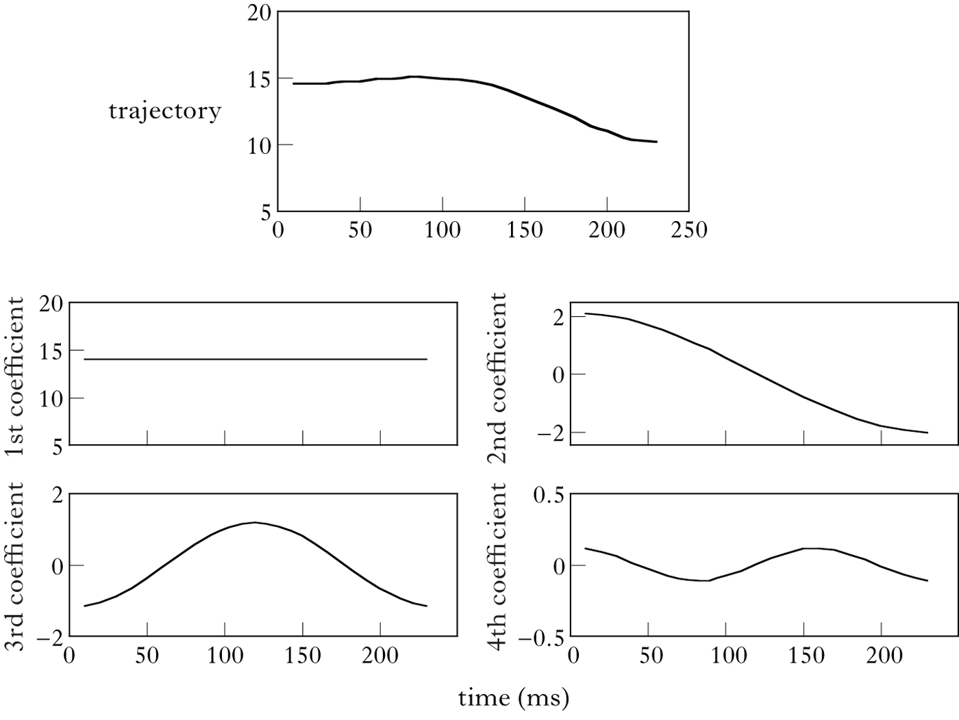
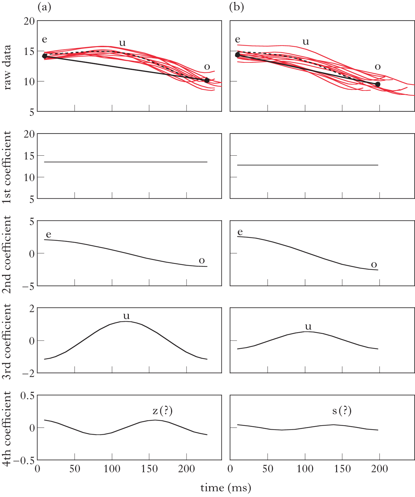
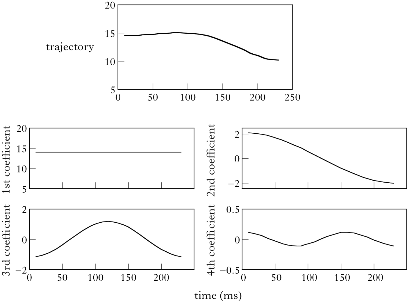
Figure 3 illustrates the DCT components of a TD trajectory. The top panel shows the trajectory, the vertical movement of the TD (y-axis) over time (x-axis). The first DCT coefficient defines a straight line at 14 mm (above the occlusal plane). In the discussion below, we refer to this line as the baseline TD height. Subsequent coefficients describe deviations from the line as cosine-shaped modulations of increasing frequency. These subsequent components are centred on zero. The second coefficient captures the downward trend of the TD trajectory, ranging from +2 mm to ―2 mm. Thus the second coefficient captures the fact that, in this data, the TD starts high and then lowers over time, and that the range of this lowering motion covers a 4 mm span. The third coefficient adds another modulation to the trajectory. Towards the middle of the trajectory there is a rise, which constitutes a modulation of the baseline trajectory of the order of ±2 mm. The effect of the fourth coefficient is much smaller, specifying modulations that are less than ±0.5 mm.
An illustration of DCT components for a TD trajectory spanning the /VCuCV/ portion of /e#ɸusoku/. The top panel shows the trajectory. The bottom four panels show individual DCT components contributing to the trajectory.
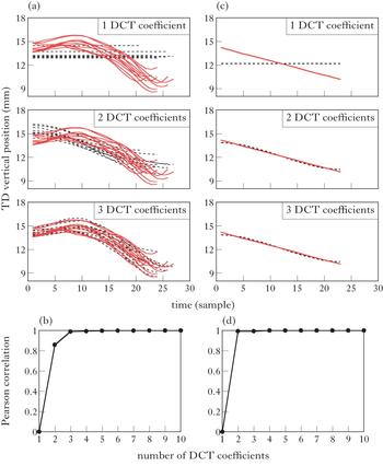
To evaluate how many cosine components are needed to represent movement trajectories in the EMA data, we simulated the TD data shown in Fig. 2 using different numbers of DCT coefficients, and evaluated changes in the degree of precision. The number of DCT coefficients was varied from one to ten. Figure 4b shows how the correlation between the raw data and the simulated data increases with the number of DCT coefficients. With just one DCT coefficient, the Pearson correlation r is nearly zero. With two coefficients, the correlation rises to 0.858, and with three it increases to 0.989. Subsequent increases in the number of DCT coefficients yield only more marginal improvement – the correlation with four coefficients is 0.992; with six it is 0.998. As illustrated here, one general advantage of the DCT analysis is that for each number of coefficients, we can generate the predicted trajectories, compare them with actual trajectories, and examine the goodness of fit. Figure 4a illustrates the goodness of fit token by token. The set of eleven /ɸuzoku/ tokens from Fig. 2 is displayed as solid lines. The dashed lines show trajectories that were simulated from DCT coefficients. With three coefficients, the solid and dashed lines overlap almost completely, illustrating nearly lossless compression of the trajectories.
(a) Raw data (solid lines) and simulated trajectories (dashed lines) for eleven tokens of the VCuCV portion of /e#ɸuzoku/. The trajectories span the /VCuCV/ interval under analysis. Simulated trajectories were based on one (top), two (middle) and three (bottom) DCT coefficients. (b) The Pearson correlation r between raw data and simulated data as a function of the number of DCT coefficients employed in data representation. (c) Linear trajectory (solid line) for the same data along with DCT components fit to the linear trajectory. (d) The correlation between the linear trajectory and trajectories simulated based on different numbers of DCT coefficients. For the linear trajectory, high precision is obtained with just two DCT coefficients.
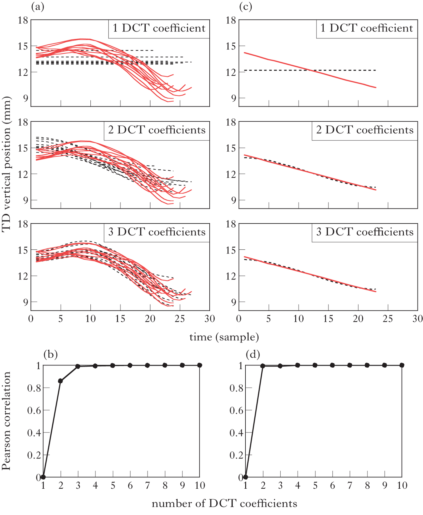
By using DCT, we can reduce the dimensionality of the data without loss of precision. Figure 4 indicates that three coefficients are sufficient to retain a detailed phonetic representation of the TD signal for the Japanese case under discussion. These DCT coefficients have plausible linguistic interpretations, on which we now elaborate.
Figure 5 displays the /ɸuzoku/ ~ /ɸusoku/ data, along with mean DCT components fitted to the data. Again, four DCT coefficients are shown. Figure 5a shows the voiced /u/ in /ɸuzoku/; Fig. 5b the devoiced /u/ in /ɸusoku/. The top panels show the raw data (solid lines) together with the average trajectory (dashed line) and a linear trajectory between /e/ and /o/ vowel (thick line). This average trajectory was computed by averaging DCT coefficients. The average trajectory is closer to the linear trajectory for /ɸusoku/ (Fig. 5b) than for /ɸuzoku/ (Fig. 5a). More importantly, each of the DCT coefficients has a plausible linguistic interpretation, which helps to isolate the difference in trajectory between voiced and voiceless vowels. The first DCT coefficient represents baseline TD height, as discussed above. The second DCT coefficient generally captures a fall in TD height from /e/ to /o/. This component is thus likely to represent the vowel-to-vowel transition, which is similar for both words. Vowel-to-vowel intervals have long provided building blocks for speech production models (Öhman Reference Öhman1966, Mrayati et al. Reference Mrayati, Carré and Guérin1988, Carré & Chennoukh Reference Carré and Chennoukh1995, Smith Reference Smith, Connell and Arvaniti1995). The third DCT coefficient represents an increase in TD height for the vowel /u/. This rise is present for both /ɸuzoku/ and /ɸusoku/, but the magnitude of the rise is greater for the voiced vowel in /ɸuzoku/ than for the devoiced vowel in /ɸusoku/. Thus the third DCT coefficient isolates the difference between these words observed in Fig. 2. Finally, the fourth DCT coefficient adds a subtle (<0.5 mm) modulation to the TD trajectory. The time course of this modulation is roughly consistent with coarticulatory effects of coronal consonants /s/ and /z/ on TD height, but is so small that it is under the average measurement error of the NDI system (Berry Reference Berry2011). We will therefore model the data with three DCT coefficients.
Average DCT components for (a) /ɸuzoku/ and (b) /ɸusoku/. The raw data is displayed in the top panels, and average DCT components are plotted in the lower panels. Only the target /VCuCV/ interval is shown.
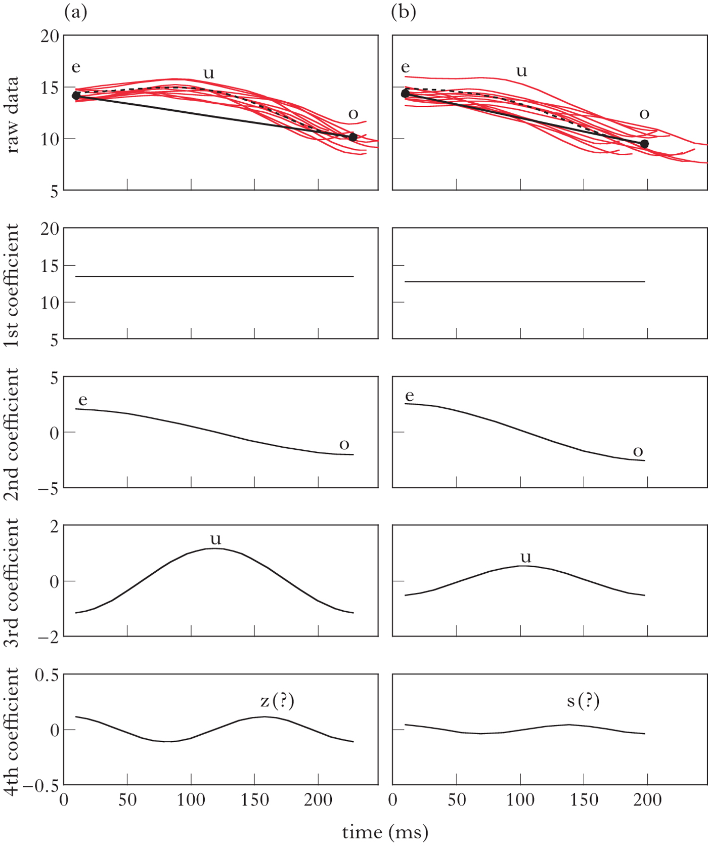
We emphasise that the decision to use three DCT coefficients for the data here was not determined a priori, but arrived at through a combination of empirical and theoretical considerations. As illustrated above, (i) using three DCT components provides a very precise representation of the data, and (ii) each component has a linguistic interpretation. Both of these criteria are important. Criterion (ii) is particularly important for constructing a stochastic representational space enabling simulation and classification of phonetic data in terms of phonological hypotheses, as it serves to evaluate whether the statistical dependencies picked up by DCT are indeed those that are a consequence of phonological control of articulation.
To summarise, the first computational step is to express TD trajectories over /VCuCV/ sequences in frequency space, as the sum of three DCT components. We next use these compressed representations of phonetic detail to estimate distributions characterising the phonetic expression of phonological form, including the no lingual target hypothesis (H3) in (1).
3.2 Stochastic sampling
The next computational tool borrows from recent stochastic approaches to modelling prosodic structure in terms of gestural timing (Shaw et al. Reference Shaw, Gafos, Hoole and Zeroual2009, Shaw & Gafos Reference Shaw and Gafos2010, Reference Shaw and Gafos2015, Shaw et al. Reference Shaw, Gafos, Hoole and Zeroual2011). These studies estimate distributions over spatio-temporally defined gestural landmarks (Gafos Reference Gafos2002), and sample from the distributions under different conditions. The parameters of such stochastic generators can be varied to test specific hypotheses about the phonological structure of the data, including the presence or absence of gestures (Shaw & Davidson Reference Shaw and Davidson2011) or the syllabic affiliation of the segments (Shaw & Gafos Reference Shaw and Gafos2010, Reference Shaw and Gafos2015). Building on the preceding section, we define Gaussian distributions over DCT coefficients instead of gestural landmarks.
Gestural landmarks and DCT coefficients both offer a sparse representation of detailed phonetic data. For the current case, an advantage of using DCT coefficients is that it is not necessary to parse specific gestural landmarks associated with the target segment.Footnote 3 Parsing gestural landmarks often relies on heuristic use of movement-velocity profiles (Shaw et al. Reference Shaw, Gafos, Hoole and Zeroual2009, Gafos et al. Reference Gafos, Hoole, Roon, Zeroual, Fougeron, Kühnert, D'Imperio and Vallée2010). In the trajectories shown in Fig. 2, however, it is not possible to identify clear velocity peaks corresponding to the different vowel gestures. Rather, the TD moves smoothly with more or less constant velocity from one vowel to the next, a pattern also reported in other kinematic data sets (e.g. Öhman Reference Öhman1966, Browman & Goldstein Reference Browman, Goldstein, Docherty and Ladd1992). In such data, selecting a single point in time that corresponds to the vowel is largely arbitrary. Our solution here is to model the entire trajectory, but in the compact and linguistically relevant form of DCT coefficients.
To formulate the no lingual target hypothesis in terms of DCT coefficients, we first fitted a straight line from V1 to V3 in /V1CuCV3/ sequences, as in the top panels of Fig. 5 (solid lines). If there is no independent TD height target for /u/ (H3), then the tongue-dorsum position should follow a smooth path from V1 to V3. To formulate a stochastic version of this targetless trajectory, we coerced the linear interpolation between vowels into frequency space by fitting three DCT coefficients to the straight line from V1 to V3. Figures 4c and d show that the linear trajectory can also be captured with high precision with a small number of DCT coefficients. We then defined distributions over those DCT coefficients. The shape of the distributions was guided by analysis of the data. We chose normal (Gaussian) distributions, since the DCT coefficients fitted to our data did not significantly depart from normality, according to Shapiro-Wilk tests. For the targetless hypothesis, the means of the distributions were the DCT coefficients fitted to the linear interpolation between vowels. The standard deviation of the distributions was set to the standard deviation of DCT coefficients fitted to the corresponding data. This ensured that we injected reasonable quantities of variation into the targetless trajectory. Formalised as distributions over the first three DCT coefficients, corresponding to the middle three panels of Fig. 5, the no lingual target hypothesis thus has the same degrees of freedom as the full vowel hypothesis, meaning that it varies in the same dimensions and to the same degree as the raw data.Footnote 4
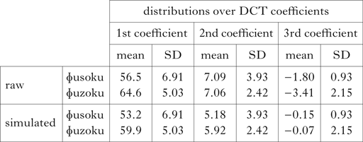
This computational method expresses the no lingual target hypothesis in the phonetic dimensions of the data, specifically the TD height over time, as phonological control of the vocal tract passes from one vowel to the next. Table I provides a specific example. The top two rows show the DCT distributions of the raw data. The mean value of each coefficient is shown, with the standard deviation. The bottom row provides the parameters for the no lingual target hypothesis for the same data. The mean parameters come from a three-parameter DCT of the straight-line trajectory, left-delimited by the mean target of V1 and right-delimited by the mean target of V3. Note that the third coefficient is nearly zero, for the targetless hypothesis, indicating no rise from the trajectory defined by the second coefficient (see also Fig. 5). The standard deviation for the no lingual target hypothesis is identical to the raw data because the level of variability in the no lingual target hypothesis is set to the level of variability in the data.
Means and standard deviations of DCT coefficients.

Having defined distributions over DCT coefficients, we can sample from the coefficients to simulate trajectories corresponding to the targetless trajectory. The sampled coefficients can then be used to specify the TD trajectory by applying the inverse DCT function to the coefficients. The formula for simulating trajectories by applying inverse DCT is given in (5). As with the DCT expression in (4), L indicates the length of the trajectory, x(n) is the trajectory, this time on the left of the equation, y(k) represents the kth DCT coefficient and w is a constant. We simulated trajectories that were equal to the mean duration of the V1 to V3 signal with k = 3 DCT coefficients.
(5)
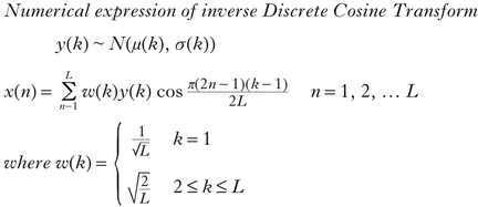
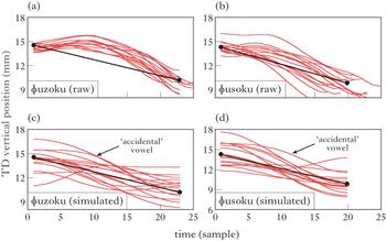
Figure 6 illustrates the simulations. For reference, the top panels re-plot the data from Fig. 2. However, as in Figs 3–5, only the portion of the trajectory beginning with the /e/ from the carrier phrase and ending with the /o/ is shown. The TD trajectories for /ɸuzoku/ are shown on the left; the trajectories for /ɸusoku/ on the right. The solid circles denote average vowel targets for V1 (/e/) and V3 (/o/). The straight line connects the means of the vowels, and defines the linear interpolation trajectory. Comparison of the left and right panels reveals that TD height in /ɸusoku/ tends to be closer to the line than TD height in /ɸuzoku/, essentially the same observation we made in Fig. 2 (but this time with reference to the linear interpolation trajectory). The bottom panels show simulated TD trajectories, sampled from the distributions of DCT coefficients given in Table I. For reference, the line denoting the linear interpolation trajectory is drawn in the lower panels as well. Note that, even though the mean of the DCT coefficients is based on the straight line, the stochastic simulations are non-linear, because the distributions over DCT coefficients define the same range of variability as is present in the TD trajectories, which are also not perfectly linear.
Top panels show actual TD data for (a) /ɸuzoku/ and (b) /ɸusoku/. (c) and (d) show simulated trajectories from the targetless hypothesis (H3 in (1)). All panels show only the target /V1CuCV2/ interval. The individual trajectories differ in length because they are delimited by the targets of V1 and V2.

In the lower panels, observe the ‘accidental’ vowels. Some of the trajectories simulated from the no lingual target hypothesis have an increase in height in the middle of the trajectory. If observed in isolation, these tokens could be misinterpreted as arising from active high vowel constrictions. The presence of ‘accidental’ vowels underscores an important point about evaluating phonological hypotheses on the basis of phonetic data, and the role of stochastic modelling. It is crucial to consider the level of variability in the data. In the case at hand, we find that amongst tokens sampled from the linear interpolation trajectory, there are some that show a rise in tongue-dorsum height at approximately the point in time that we would expect the vocal tract to be under control of a vowel gesture; however, such ‘accidental vowels’ simply arise from noise in the data, which should not be confused with phonologically specified targets. The presence of accidental vowels in the simulations indicates that the level of normal variation that characterises fluent production of a native language is of the order of magnitude of the presence or absence of a vowel in one or two out of a dozen or so tokens.
We can now statistically adjudicate between three of our four hypotheses in (1). In asking whether the vowel is targetless, we are essentially asking whether the TD rise in the middle of the trajectory is greater than can be expected by chance. We have defined chance for /ɸusoku/ as the noisy targetless trajectory in Fig. 6. Using sparse representation of the data, as in (2), we can statistically compare /ɸusoku/ to /ɸuzoku/ to examine whether the TD trajectory in the devoiced vowel differs from that in the voiced vowel. This constitutes a direct statistical test of H1, the hypothesis that devoiced vowels are the same as the voiced counterparts. A significant difference would falsify H1, leaving us with hypotheses H2 and H3, i.e. that the lingual gesture in devoiced vowels is either reduced or deleted. Further, we can compare the TD trajectory in /ɸusoku/ to the simulated targetless trajectory, to test whether the data differs significantly from linear interpolation. This constitutes a statistical test of H3. A significant difference would leave us with H2 as the only viable alternative. However, this method does not allow us to test H4, the optional lingual target hypothesis. The reason is that, in evaluating statistical significance in this way, we are testing whether the tokens as a group are different, which involves the implicit assumption of phonological homogeneity across tokens of a word (see Bayles et al. Reference Bayles, Kaplan and Kaplan2016). The next computational tool we introduce alleviates this problem. However, if it can be ensured that a phonological process is not optional, then DCT together with micro-prosodic sampling should suffice to provide a rigorous assessment of smooth interpolation.
4 Classification
Many phonological processes are optional. Capturing the variability requires a probabilistic phonological model (Anttila Reference Anttila and Hinskens1997, Boersma & Hayes Reference Boersma and Hayes2001, Coetzee & Kawahara Reference Coetzee and Kawahara2013). In these models, phonetic reduction and variable targetlessness are completely different scenarios. The latter requires stochastic interpretations of constraint rankings (or rules); the former requires continuous phonological representations of some sort (e.g. Smolensky et al. Reference Smolensky, Goldrick and Mathis2014). To distinguish between these possibilities, we make use of the distributions built for simulation to classify phonetic data in terms of phonological structure. For this purpose, we use a naive Bayesian classifier, which will allow us to analyse the data token-by-token without committing ourselves to the assumption that the surface phonological form of a word is uniform and invariant.
The Bayesian classifier assigns the probability of category membership. Importantly, it does so for each test token separately. For the case at hand, we use the DCT representation (with three coefficients) as input to the classifier. The output is the probability of whether the articulatory target in that token comes from the ‘full lingual target’ category or the ‘no lingual target’ category. The DCT coefficients that describe the data are statistically independent, which makes them appropriate dimensions for the naive Bayesian classifier. The formula is provided in (6).Footnote 5
(6)

The output of the formula, i.e. p(T | Co 1, …, Co n) is the posterior probability of targetlessness, which designates the probability of a targetless articulation, given the DCT coefficients. The alternative to a targetless articulation is that there is a full vowel target present. The posterior probability of a vowel target is calculated from a prior probability of targetlessness and the probability of the DCT values given the category. The prior probability of targetlessness is the term p(T). The probability of the DCT values given the category is the term in (7a). This is calculated on the basis of the training data, and is normalised by a third term, (7b), the probability of the DCT coefficients in the whole dataset.
(7)

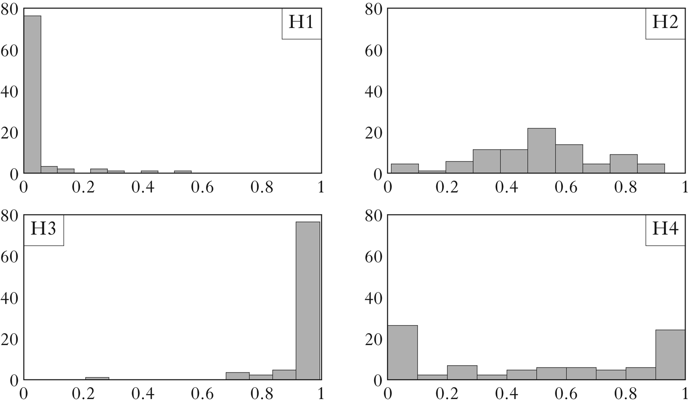
In this particular case, we are concerned with assessing the four hypotheses in (1) on the basis of the phonetic signal. To give each hypothesis equal weight, we assign equal prior probabilities to the categories full lingual target, H1 in (1), and no lingual target, H3 in (1). Thus p(T) is set to 0.5.Footnote 6 The other hypotheses, vowel reduction (H2) and variable targetlessness (H4), can also be evaluated on the basis of posterior probability patterns, as we illustrate below in Fig. 8.
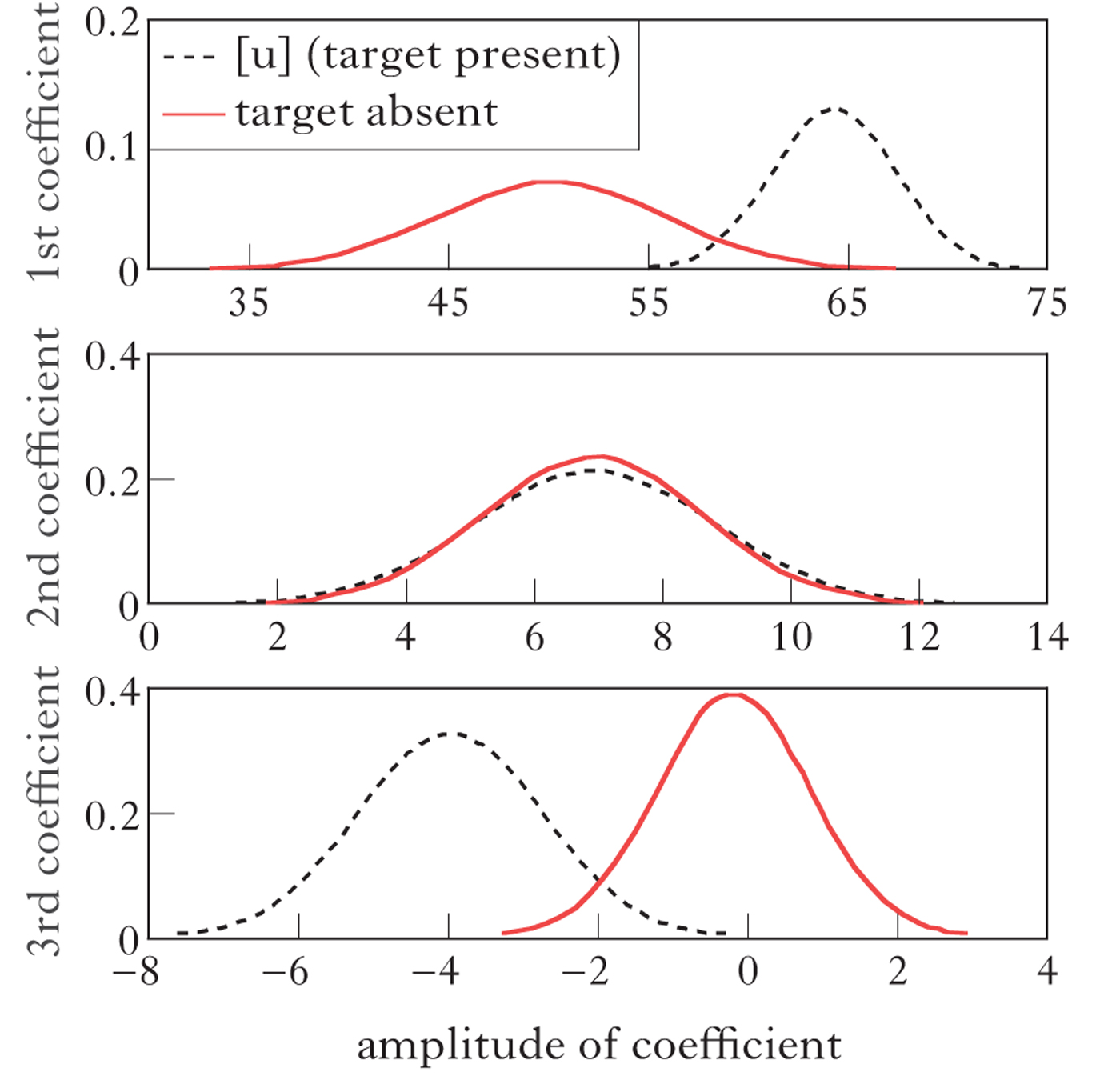
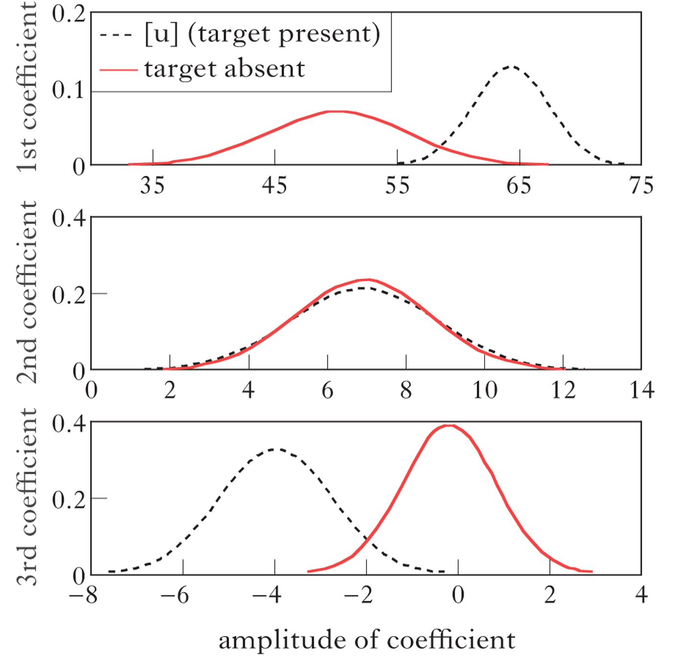
We trained the Bayesian classifier on two sets of three DCT coefficients. The full lingual target data came from DCT coefficients fitted to tokens of /ɸuzoku/. The no lingual target data came from DCT coefficients fitted to the linear interpolation trajectory from /e/ to /o/ (as in Figs 6c and d). Since we have set the prior probability to even odds of targetlessness, it is the probability of each DCT coefficient given the presence/absence of a TD height target (the term in (7a)) that dictates posterior probabilities. To illustrate this, Fig. 7 compares Probability Density Functions (PDFs) across the full lingual target vs. no lingual target hypotheses for each DCT coefficient. The dashed lines show PDFs over the baseline (full lingual target) hypothesis, based on [ɸuzoku] tokens; the solid lines show the no lingual target hypothesis, based on noisy simulation of linear interpolation. As can be seen from Fig. 7, the PDF of the second DCT coefficient is heavily overlapped. The main differences between the presence and absence of a vowel are found in the PDF of the first and third coefficients. This is expected, since the first coefficient is related to the average TD height across the trajectory and the third coefficient dictates the magnitude of the TD rise between /e/ and /o/ (see Fig. 5). Thus the parameters of the Bayesian classifier for /ɸusoku/ give quantitative probabilistic form to the observations we have already made about the data.
The probability distribution functions for DCT coefficients, given the no lingual target hypothesis and the alternative full lingual target hypothesis, based on the data in Fig. 2.
Four possible patterns, displayed as histograms over posterior probabilities of targetlessness, are illustrated in Fig. 8. These hypothetical results correspond to the four hypotheses in (1). The histogram in Fig. 8a was obtained by submitting /ɸuzoku/ tokens (from six speakers) to the Bayesian classifier. As expected, most of these tokens have greater than 0.95 probability of containing a vowel, although there are a few tokens with lower probabilities. This pattern corresponds to H1, that the lingual gestures for voiced vowels are the same as for voiceless vowels. The histogram in Fig. 8b was obtained by submitting the same number of simulated ‘vowel absent’ trajectories to the classifier. Again, as expected, most tokens have a 0.95 or greater probability of targetlessness, although there are a few tokens with lower probabilities, and one ‘accidental vowel’, which has a lowish (0.25) probability of targetlessness. This pattern corresponds to H3, that the lingual gestures of devoiced vowels have no target. The third pattern, illustrated in Fig. 8c, shows posterior probabilities for reduced vowels (H2). These were generated by stochastic sampling of DCT coefficients that were averaged between full lingual target (H1) and no lingual target (H3) values. Thus, quite literally, the reduced vowel cases are intermediate trajectories between the fully articulated vowel and the targetless vowel. The fourth pattern, representing H4, is the variable targetlessness pattern. We created this pattern by sampling at random from distributions characterising the full lingual target and the no lingual target data.
The four hypothetical posterior probability patterns in (1): H1 (full lingual target); H2 (reduced lingual target); H3 (no lingual target); H4 (optional lingual target). The x axis of each histogram shows posterior probabilities generated by the Bayesian classifier summarised in Fig. 7. See Appendix A for different instantiations of H2 which assume different degrees of variability.

5 Results
5.1 Simulation results
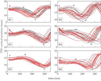
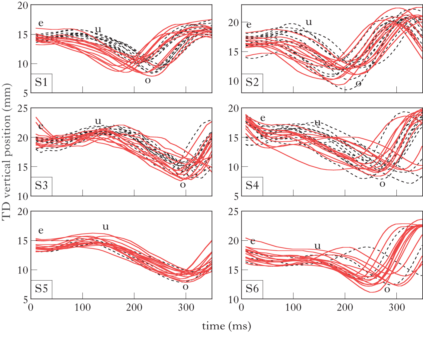
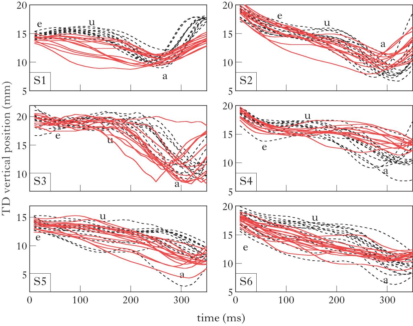
Figure 9 shows the TD height trajectory in /ɸusoku/ and /ɸuzoku/ for all six speakers. Solid lines show change in TD height over time for /ɸusoku/; dashed lines show /ɸuzoku/. The TD height trajectories begin with the /e/ of the carrier phrase and continue for 340 ms. The dip in the trajectories corresponds to lowering of the TD for the vowel /o/. This is followed by a rise of the TD for /k/ at the ends of the trajectories. There is variation across speakers in the degree to which the two types of line overlap. They are very closely overlapped for S5 and S6, but less so for other speakers. As described in the methods, only the portion of the trajectory from /e/ to /o/ was included in subsequent analysis.
Change in TD height (y-axis) over time for /ɸusoku/ (solid lines) and /ɸuzoku/ (dashed lines). The figure shows a fixed window beginning with the /e/ of the carrier phrase and extending for 340 ms, which is longer than the analysis window (for most tokens a rise in TD height for /k/ can be observed following the TD minima for /o/).
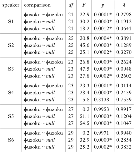
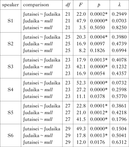
Following the method introduced in §3, we fitted DCT coefficients to each TD height trajectory, and defined a targetless trajectory. We then compared DCT components, using MANOVA. For each speaker, we evaluated the effect of voicing on the TD trajectory as well as differences between the actual trajectories and the targetless trajectory. The results are summarised in Table II. Since the targetless trajectory is stochastically sampled, statistical comparisons vary depending on the particular sample. To ensure stable and replicable MANOVA results, we report the average across ten independent simulations of the targetless trajectory. Since we conducted these analyses for each speaker and each pair of items separately, we adjusted the alpha level to correct for multiple comparisons. The Bonferroni corrected alpha is 0.00138 (0.05/36), where 36 is the total number of comparisons: 6 speakers × 2 item pairs × 3 comparisons per item pair.
MANOVA results for /ɸusoku/ and /ɸuzoku/ for each speaker.
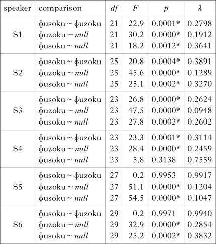
In Table II, significant differences are indicated by asterisks. Of the six participants, four produced reliable differences between the vowels in /ɸusoku/ and /ɸuzoku/. For all six participants, the voiced vowel in /ɸuzoku/ differed significantly from the targetless trajectory. Of the four speakers who produced /ɸusoku/ and /ɸuzoku/ differently, only one, S4, produced the devoiced vowel in /ɸusoku/ consistent with the targetless trajectory; for the other three, it was significantly different.
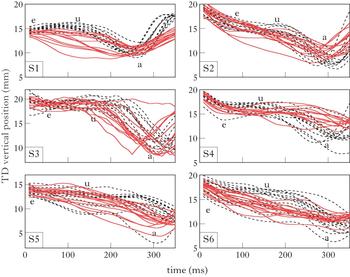
Fig. 10 shows the trajectory of TD height for another pair of words, /ʃutaisei/ and /ʃudaika/. The solid lines show the word containing the devoiced vowel, /ʃutaisei/; the dashed lines show the comparison word, /ʃudaika/, which contains a voiced /u/. For all six speakers, the TD trajectory is somewhat lower for the devoiced vowel than for the voiced vowel. Moreover, for several speakers the solid lines have an almost linear trajectory between the flanking vowels /e/ and /a/. To assess the statistical significance of these trends we fitted DCT components to each trajectory, simulated a targetless trajectory and compared these via MANOVA. The results are given in Table III.
Change in TD height (y-axis) over time for /∫utaisei/ (solid lines) and /∫udaika/ (dashed lines). The figure shows a fixed window beginning with the /e/ of the carrier phrase.
MANOVA results for /∫utaisei/ and /∫udaika/ for each speaker.

As shown in Table III, all six speakers produced /ʃutaisei/ and /ʃudaika/ with significantly different TD trajectories. Moreover, of the six speakers, only one, S5, produced /ʃutaisei/ differently from the targetless trajectory. For completeness, we also note that one speaker, S2, who did not produce a difference between /ʃutaisei/ and the targetless trajectory, also did not produce a difference between /ʃudaika/ and the targetless trajectory that was significant after Bonferroni correction (p = 0.009, where α = 0.001).
To summarise, most speakers showed significant differences in tongue-height trajectories between voiced and voiceless vowels. This result allows us to rule out the possibility that devoiced vowels are produced with the same lingual articulatory gestures as voiced vowels, as predicted by H1 in (1). With respect to targetlessness, the statistical evaluation indicates that /u/ may sometimes be targetless.Footnote 7 One speaker, S4, produced /ɸusoku/ and five speakers produced /ʃutaisei/ without a clear height target. Thus a conclusion based on this analysis is that devoiced vowels are often reduced, and sometimes even produced without a target. We would have to divide speakers into three groups based on /ɸusoku/, those who produce /u/ without a height target (S4), those who reduce /u/ (S1–S3) and those who produce full vowels (S5–S6), but into just two groups based on /ʃutaisei/, those who reduce (S5) and those who produce a targetless /u/ (S1–S4, S6). We caution, however, that analysis by MANOVA treats as a homogenous group all tokens of /ɸusoku/ and /ʃutaisei/ for a given speaker. If there is within-speaker optionality, then this assumption is not justified. We next turn to phonological classification of the data on a token-by-token basis. This approach will evaluate the optional lingual target hypothesis (H4), and offer additional insights into the other hypotheses.
5.2 Classification results
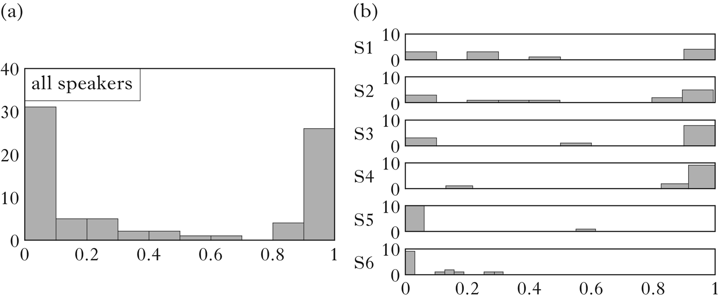
We submitted each token of /ɸusoku/ and /ʃutaisei/ in Figs 9 and 10 to a Bayesian classifier, as described in §4. Recall that, as illustrated in Fig. 8, all four hypotheses in (1) can be expressed as patterns of posterior probabilities, the output of the Bayesian classifier. For easy comparison with Fig. 8, we summarise the posterior probabilities as histograms.
Figure 11 provides a histogram for /ɸusoku/. (a) aggregates across speakers, and (b) provides a breakdown by speaker. The pattern clearly shows that there are two modes in the probabilities. One of them is around 0.05 probability of targetlessness; the other is around 0.95 probability of targetlessness. In fact, there are very few tokens at all that have intermediate probabilities, i.e. tokens which we could call phonetically reduced. Across the six speakers, rather, it seems that /u/ in /ɸusoku/ is optionally targetless. The breakdown of individual speakers in (b) helps us to make sense of the MANOVA results. Recall that speakers S1–S3 showed significant differences between /ɸusoku/ and /ɸuzoku/, as well as between /ɸusoku/ and the targetless trajectory. Figure 11b makes clear why this is: these speakers optionally produce the vowel without a height target. The same is true for S4, who was put into a different group based on the MANOVA results. The main difference amongst speakers S1–S4, therefore, is not between phonetic reduction and phonological targetlessness, but rather in the frequency with which the vowel is targetless. The other speakers, S5 and S6, produced no tokens that were classified as targetless. S5 had just one reduced token, with a targetless probability of 0.6; S6's most reduced token had a targetless probability of just 0.3.
Posterior probabilities of targetlessness for 77 tokens of /ɸusoku/ from six speakers (the TD trajectories shown in Fig. 9). (a) aggregates across speakers; (b) probabilities by speaker.

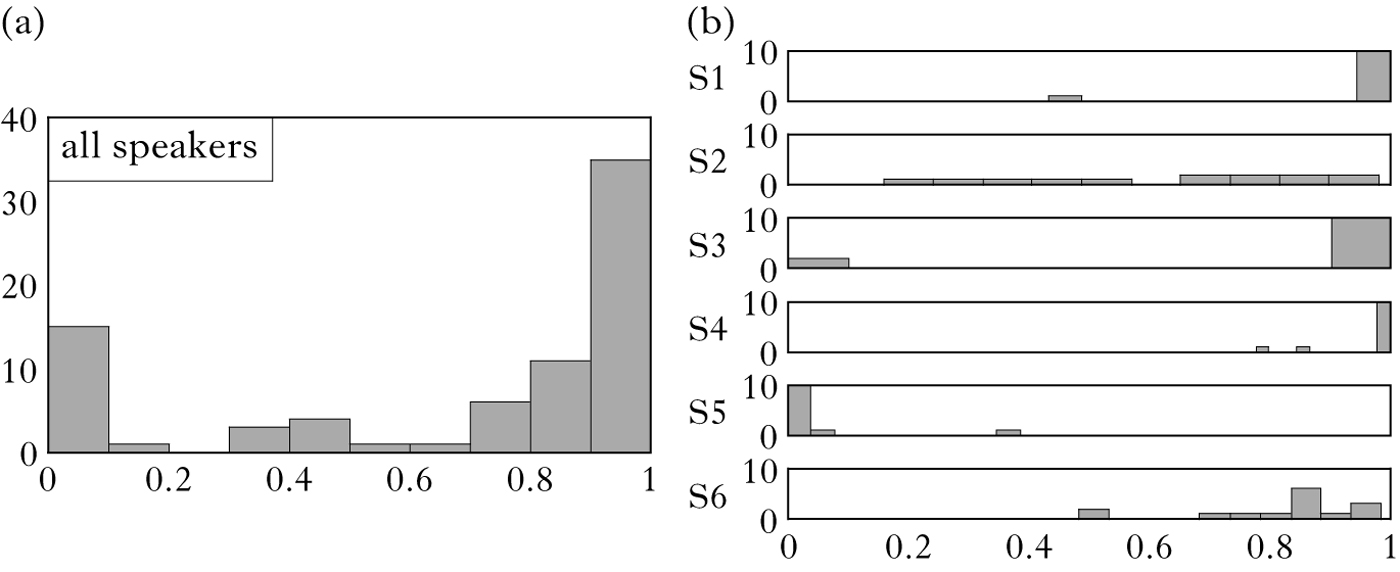
Figure 12 provides similar histograms for /ʃutaisei/. Again, the pattern in the posterior probabilities is bimodal, with one peak at a high probability of targetlessness and the other at a very low probability of targetlessness. Just as in /ɸusoku/, the vowel /u/ in /ʃutaisei/ is produced with an optional target. It is noticeable that there are no tokens that are intermediate between the full vowel and the linear interpolation trajectory. The subject-level data (Fig. 12b) shows that just one speaker, S2, is prone to gradient reduction. Apart from S2, the other speakers produce only a small number of tokens (three) in the ambiguous 0.3 to 0.7 probability range. Consistent with the MANOVA results, the individual speaker results indicate that five speakers (including S2) tend to produce the /u/ in /ʃutaisei/ without a vowel-height target, while one speaker, S5, reliably produces the word with a vowel-height target.
Posterior probabilities of targetlessness for 77 tokens of /ɸutaisei/ from six speakers (the TD trajectories shown in Fig. 10). (a) aggregates across speakers; (b) probabilities by speaker.

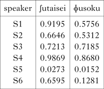
The Bayesian classification provides converging evidence for some of the conclusions based on MANOVAs, but also additional insights. Both analyses indicate that targetlessness is more common in /ʃutaisei/ than in /ɸusoku/. Table IV shows that this holds true for every speaker: although targetlessness varies across speakers, all of them show a higher probability of targetlessness in /ʃutaisei/ than in /ɸusoku/. This holds even for S5, who has a low probability of targetlessness in both words. The MANOVA analysis also indicates that targetlessness is more common in /ʃutaisei/ than in /ɸusoku/; Bayesian classification reveals that this holds across all speakers individually as well. Thus, while the overall probability of targetlessness seems to be a matter of personal preference, relative probabilities of targetlessness are shared across speakers.
Average probability of targetlessness by speaker and by word.

Another new insight gained from Bayesian classification is the status of H2 in (1). When comparing DCT components via MANOVA, we found that four out of six speakers showed significant differences between voiced (/ɸuzoku/) and voiceless (/ɸusoku/) contexts. Of these four speakers, three also showed a significant difference between /ɸusoku/ and the targetless trajectory. Since the productions of /ɸusoku/ differ as a group both from /ɸuzoku/ and from linear interpolation, we might be tempted to conclude that the vowels are reduced but not targetless. The Bayesian classification reveals that this conclusion is unwarranted. Rather, a group of /ɸusoku/ tokens from a single speaker may be different from both the full vowel trajectory in /ɸuzoku/ and the targetless trajectory because it contains a mix of full vowel and targetless tokens. The Bayesian classification reveals that this is indeed the case for /ɸusoku/. Production of a lingual target in devoiced vowels in Tokyo Japanese is optional, but phonetic reduction is rare. Tokens are either produced with a full vowel, similar to the voiced context, or with no lingual vowel target at all, as in the linear interpolation assumed for tokens that lack a vowel in the surface representation.
6 Discussion
6.1 Summary
We have illustrated a computational approach to assessing surface phonological form based on phonetic data. The general strategy was to develop a stochastic representational space that links discrete phonological form to continuous phonetic data through simulation and classification. Our specific proposal was to express phonological hypotheses in terms of distributions over harmonic (frequency) components, extracted using DCT. We showed that DCT compresses the phonetic data into a small number of phonologically relevant parameters, which preserve phonetic detail. As a proxy for phonetic interpolation, we defined a linear trajectory between flanking vowels in this DCT frequency space. Stochastic sampling from distributions over DCT coefficients enabled simulation of competing phonological hypotheses (full lingual target vs. no lingual target) with the level of phonetic variability observed in the data. Finally, we used the distributions to assign probabilities of targetlessness to unseen data, according to Bayes’ rule. We illustrated the method with TD movements produced by Tokyo Japanese speakers as a case study. Based on existing literature, we motivated four possible hypotheses about lingual articulatory targets, and demonstrated step by step how our computational approach can adjudicate between them.
6.2 What we have learned about high vowel devoicing
Results for Tokyo Japanese indicate that the lingual articulatory gesture of devoiced vowels is rarely reduced, despite the fact that, given the devoicing, it can have only negligible auditory consequences. There are, however, two distinct phonetic outcomes for devoiced vowels. They can be produced with or without a vowel-height target. This result supports H4 in (1), the hypothesis that devoiced vowels have an optional lingual target.
Another interesting aspect of the results is that the probability of vowel targetlessness varied systematically across the pair of words examined. For all speakers, the probability of producing a vowel without a height target was higher for /ʃutaisei/ than for /ɸusoku/. This difference could be due to resulting consonant-cluster phonotactics. Deletion of /u/ in /ʃutaisei/ would give rise to a fricative–stop cluster, [ʃt], which may be a better surface form than the fricative–fricative cluster [ɸs] resulting from /u/-deletion in /ɸusoku/. If we assume that a syllable boundary remains between these surface consonants (for evidence that it does, see Shaw & Kawahara Reference Shaw, Kawahara, Gallagher, Gouskova and Yin2018a), a preference for fricative–stop clusters over fricative–fricative clusters follows from syllable-contact laws (e.g. Vennemann Reference Vennemann1988). Since there is a greater decrease in sonority between the offset of one syllable and the onset of the next, [ʃ.t] is less marked than [ɸ.s] (Gouskova Reference Gouskova2004). It is not clear exactly what other facts of Japanese, if any, motivate this fine-grained grammatical preference, although similar types of patterns have been observed in the production and perception of unfamiliar consonant clusters (e.g. Berent et al. Reference Berent, Steriade, Lennertz and Vaknin2007, Berent et al. Reference Berent, Lennertz, Smolensky and Vaknin-Nusbaum2009, Davidson & Shaw Reference Davidson and Shaw2012).
Consistency across speakers in the relative targetlessness of /ʃutaisei/ and /ɸusoku/ resembles other well-studied cases of phonological variation, such as t/d-deletion, in which grammatical influences remain constant even as overall deletion rates vary across speakers (Guy Reference Guy and Hinskens1997, Coetzee & Kawahara Reference Coetzee and Kawahara2013). Some additional discussion of possible factors influencing deletion can be found in Shaw & Kawahara (Reference Shaw and Kawahara2018b), where the analysis developed here is extended to more words, and presented alongside converging phonetic evidence for variable deletion of lingual articulatory targets.
6.3 Comparison with other approaches
Our approach differs from other quantitative attempts to assess phonological hypotheses, including targetlessness, on the basis of phonetic data. To highlight its unique points, we briefly summarise previous approaches, which can be divided into four categories: (i) the heuristic use of phonetics, (ii) statistical comparison of two samples of phonetic data, (iii) the prediction of one part of the phonetic signal from another and (iv) hypothesis testing by simulation.
The first approach, the heuristic use of phonetics, involves drawing some conclusion about phonological form on the basis of visual inspection of the phonetic signal. Phonetic heuristics have played an important role in foundational work in laboratory phonology, including in the context of arguing for phonetic underspecification (Keating Reference Keating1988, Cohn Reference Cohn1993). They can be useful in augmenting auditory impressions of phonological form, particularly from researchers who are non-native speakers of the target language. However, phonetic heuristics may also break down. They are sometimes too sensitive, and sometimes not sensitive enough. Consider, for example, a common phonetic heuristic for a vowel between stop consonants: ‘a period of voicing … with formant structure containing a visible second formant that ended with abrupt lowering of intensity at the onset of the second stop’ (Davidson Reference Davidson2010). Application of this heuristic to Tashlhiyt Berber, for example, greatly overestimates the frequency of vowels in the language (Ridouane Reference Ridouane2008). A Berber word such as /t-bdg/ ‘it is wet’ contains no vowels in the phonological representation, but is normally pronounced with three periods of voicing that would meet the phonetic heuristic above (Ridouane & Fougeron Reference Ridouane and Fougeron2011). In this case, the phonetic heuristic is too sensitive. On the other hand, English words such as support, which contain two phonological vowels, are sometimes produced with just one vocalic interval, meeting the above heuristic for a vowel (Davidson Reference Davidson2006b). In this case, the phonetic heuristic is not sensitive enough. Heuristics break down because they do not capture the full range of phonetic signals consistent with phonological form.
An alternative to the visual inspection of the phonetic signal is to statistically compare one or more phonetic dimensions in two groups of words that are hypothesised to differ in phonological structure. A wide range of statistical tools have been deployed to this end (see e.g. Davidson Reference Davidson2006a, Lee et al. Reference Lee, Byrd and Krivokapić2006, Wieling et al. Reference Wieling, Tomaschek, Arnold, Tiede, Bröker, Thiele, Wood and Baayen2016). For example, SSANOVAs can be used to compare populations of splines (Gu Reference Gu2013), such as tongue shapes, TD trajectories or even more complex derived variables (e.g. change in tongue curvature over time; Ying et al. Reference Ying, Carignan, Shaw, Proctor, Derrick and Best2017), and have been applied to various phonetic signals (Davidson Reference Davidson2006a). Similarly, Functional Data Analysis (FDA) fits a series of splines to time aligned signals, and has been shown to differentiate temporal differences associated with prosodic context (Lee et al. Reference Lee, Byrd and Krivokapić2006). Another approach uses Generalised Additive Models, which have been developed to support random effects, e.g. of talker. Generalised Additive Models have recently been applied to EMA data, detecting dialect variation on the basis of movement trajectories from large samples of speakers (Wieling et al. Reference Wieling, Tomaschek, Arnold, Tiede, Bröker, Thiele, Wood and Baayen2016). These techniques can all be used to assess significant differences between populations of trajectories, such as those produced in different prosodic contexts or by speakers of different regional accents. However, a significant difference between two populations of signals does not necessarily indicate the nature of the phonological difference. As our case study demonstrates, the same word can be produced with different phonological specifications. Populations of signals can therefore be different not because they actuate different phonological structures, but because they actuate different combinations of phonological structures (also Shaw & Davidson Reference Shaw and Davidson2011). Alternatively, populations of signals can differ due to phonetic factors. For example, Shaw et al. (Reference Shaw, Chen, Proctor and Derrick2016) demonstrate that tongue height in Mandarin Chinese vowel production varies across tones. Despite the common claim that tones and vowels are phonologically independent (e.g. Yip Reference Yip2002), there are dependencies between laryngeal and supralaryngeal articulation that result in small but statistically significant subcategorical differences in lingual articulation for the same vowel produced with different tones. Thus statistical differences between surface measurements offer no guarantee of a categorical phonological difference between samples. As with the heuristic use of phonetics, statistical comparison of continuous dimensions can be oversensitive, picking up differences that do not correspond to phonological structure (or to phonological differences of theoretical interest).
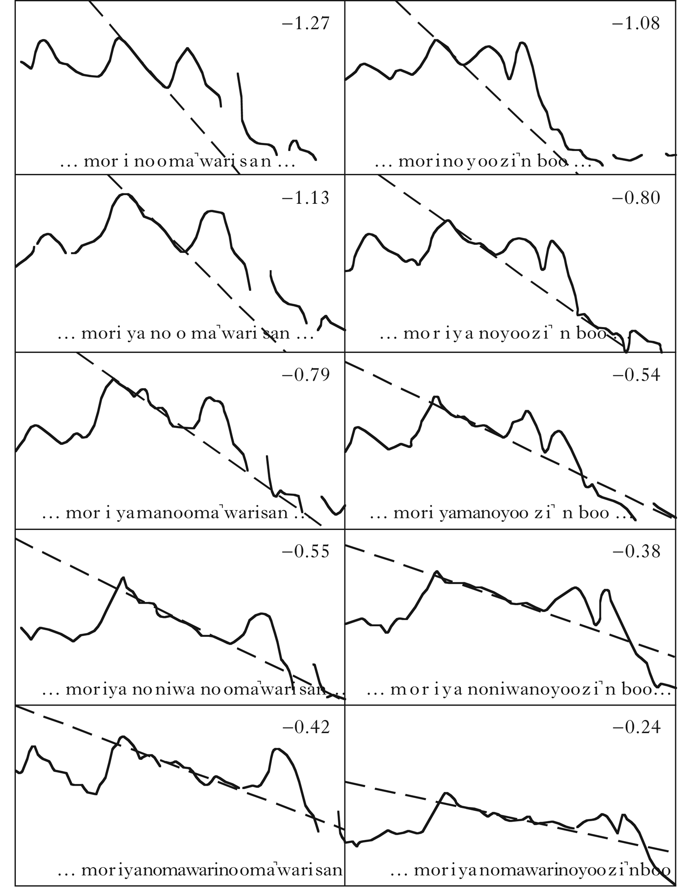
A third approach is to use one part of the phonetic signal to predict another. For example, Pierrehumbert & Beckman (Reference Pierrehumbert and Beckman1988: 37–38) rely on this approach to argue for sparse tonal specifications in Japanese unaccented words. They argue that in unaccented words only the first two syllables are specified as LH. Because following syllables are unspecified, there is a general decline in F0 toward the L tone in the next Accentual Phrase. They show that the longer the duration between H and L, the shallower the slope of the F0. Figure 13 is based on their illustrative figure. In this case, the duration between H and L tones is used to predict the slope of the F0 fall. The relationship between these phonetic variables, number of intervening syllables and the slope of the F0 fall constitutes an argument for the tonal targetlessness of intervening syllables.
An illustrative figure based on Pierrehumbert & Beckman (1988), which was used to argue for tonal underspecification. There is a correlation between the temporal duration between the H tone and the L tone and the slope of a line fitted to the F0 contour. The numbers in each panel denote the steepness of the slope.

This specific correlation requires manipulating the duration of the hypothesised ‘targetless’ material, which may not always be possible, but conceptually similar approaches have been applied to other arguments for targetlessness.Footnote 8 Browman & Goldstein (Reference Browman, Goldstein, Docherty and Ladd1992) use a multiple regression framework to assess whether English schwa contains an articulatory target. They reason that schwa can be claimed to be targetless in sequences such as /pV1pəpV2p/ if the spatial position of the articulators can be reliably predicted by the flanking vowels in a two-parameter (one coefficient for each flanking vowel) linear regression model (also Lammert et al. Reference Lammert, Goldstein, Ramanarayanan and Narayanan2014). They argue that schwa in such words has a target of its own, since regression models with an intercept term, representing the mean height of the signal, tended to outperform models informed only by flanking vowel positions. This same approach has been generalised to assess vowel specification on the basis of formant trajectories (Choi Reference Choi1995). Choi demonstrates that the F2 of Marshallese vowels can be predicted from flanking consonants, and argues that they are therefore unspecified for backness.
In modelling contextual effects on English schwa, Browman & Goldstein (Reference Browman, Goldstein, Docherty and Ladd1992) also deploy what we consider to be a fourth type of approach. They simulated phonetic data from various phonological hypotheses, including targetlessness, and compared the simulated data to the experimental data. They found a qualitative match between simulated data and experimental data when English schwa is specified in the model with a neutral vowel target and overlapped in time with the following vowel, a result that converges nicely with the regression analysis described above, and makes different predictions than the targetless specification (particularly in high vowel environments). Browman & Goldstein explore several possible phonological configurations by specifying gestural scores by hand and examining the phonetic consequences. More recent simulations derive gestural scores from coupled oscillators (Saltzman et al. Reference Saltzman, Nam, Krivokapić and Goldstein2008) or posit coordination topologies isomorphic with syllable structure while fitting lower-level parameters to the data (Shaw & Gafos Reference Shaw and Gafos2010, Reference Shaw and Gafos2015, Gafos et al. Reference Gafos, Charlow, Shaw and Hoole2014). The computational toolkit we have introduced belongs to this fourth type of approach, which assesses competing phonological hypotheses computationally, by simulating those hypotheses in the physical dimensions of phonetic data. This can of course be combined with other methods described above. For example, in their investigation of the effects of prosodic structure on articulation, Parrell et al. (Reference Parrell, Lee and Byrd2013) first simulated trajectories from the TaDA articulatory synthesiser under different prosodic conditions. They tested their FDA-based measure of prosodically dictated temporal modulation on the simulated data to verify that it picked up the a priori known prosodic differences before extending the measure to investigate prosodic effects in naturally produced speech. Like our approach, this method relies on phonologically informed simulation to guide statistical analysis of the data in terms of phonological structure.
In comparison with other models instantiating the fourth class of approaches described above, our toolkit is in some ways more bottom-up, requiring fewer theoretical commitments and also fewer researcher degrees of freedom.Footnote 9 First, the parameters in the model, i.e. the values of the DCT coefficients, are determined by the data, according to the algorithm in (4). Second, our approach does not privilege particular points in time as having greater phonological relevance than others. In many of the studies described above, specific moments in time are selected for analysis. For example, Browman & Goldstein (Reference Browman, Goldstein, Docherty and Ladd1992), Shaw et al. (Reference Shaw, Chen, Proctor and Derrick2016) and Blackwood Ximenes et al. (Reference Blackwood Ximenes, Shaw and Carignan2017) select, by automatic algorithm, a specific point in time to represent the spatial position of a vowel. Regardless of whether the algorithm is based on displacement of articulators, formant values, minimum/maximum velocity, the temporal midpoint of voicing, etc., ‘target’ selection introduces a researcher degree of freedom. Our toolkit alleviates the necessity of picking points in time associated with the target phonological structure. This aspect of the approach is particularly useful for addressing the presence/absence of a target, as it is problematic to choose a point in time corresponding to a target that might not be there. Thus our approach makes the presence or absence of targets a largely empirical question, which can be addressed with phonetic data. One assumption that we have adopted here is that targetlessness corresponds to linear interpolation in the phonetics. Beyond this, since the parameters capturing phonetic signal modulation are fitted to the data quantitatively, the bottom-up approach remains compatible with most higher-level theories of phonological representation, including dynamically defined gestural units, as in Articulatory Phonology. Perhaps most importantly, the number of parameters in our representation of the signal is small, and each has a phonological interpretation. This property contrasts with GAMs, FDA and other powerful algorithms capable of fitting non-linear data, and, in particular, it facilitates a phonological interpretation of the phonetic signal.
6.4 Broader applications
Although the computational toolkit we have assembled to assess interpolation takes continuous phonetic data as input, the results for devoiced vowels in Japanese are remarkably categorical. Most tokens are either produced without a vowel target or with a full vowel target. The approach does not dictate such categorical outcomes (see Fig. 8 and Appendix A). With respect to deletion of high vowels in Japanese, the categorical nature of the variation, as revealed by application of our approach, and its interaction with other grammatical factors suggest that the phenomenon has a distinctly phonological character. Although there is a long line of research on formal architectures that can model variable phonological processes (for an overview, see Coetzee & Pater Reference Coetzee, Pater, Goldsmith, Riggle and Yu2011), the development of formal tools for assessing whether the data require a phonological solution has lagged behind. We are optimistic about the prospects of applying our computational toolkit to a wider variety of phenomena, and curious about the extent to which other cases of ‘phonetic reduction’ are actually manifestations of optional phonological processes.Footnote 10 We hope that the proposed toolkit will be used broadly in reassessing alleged cases of reduction to test whether they should be modelled as reduction or as optional processes of phonological deletion/targetlessness.
As discussed in the introduction, the toolkit is designed to address the general issue of phonetic underspecification, whether the source is phonological deletion or lexical underspecification or non-specification. One domain within which the current toolkit may be particularly applicable is intonation. As mentioned in the introduction, the issue of underspecification (targetlessness) is particularly important in the domain of intonation, because the dominant analytical framework of intonation, the autosegmental/metrical model of intonation, generally assumes sparse tonal specification (see Xu et al. Reference Xu, Lee, Prom-on and Liu2015 vs. Arvaniti & Ladd Reference Arvaniti and Ladd2015 for a recent exchange of opinions on this matter). Since intonation, just like the articulatory data reported here, comes with much natural variability, including individual variation, application of these tools to the tonal underspecification hypothesis may prove to be informative. For example, the trade-off between signal length and F0 slope identified by Pierrehumbert & Beckman (Reference Pierrehumbert and Beckman1988) and shown in Fig. 13 is a natural consequence of DCT, since the amplitude of DCT components are inversely related to the length of the signal (see (4), where y(k) is amplitude and L is signal length). Moreover, there are some ‘bumps’ on the ‘linear’ F0 trajectories, which could be due either to non-linguistic perturbations of the signal or phonological specifications, precisely the type of distinction that can be addressed in our framework.
In closing this section on the broader applicability of our approach, we would like to summarise aspects of our analysis that we expect will vary depending on the specific dataset being analysed. We chose three DCT coefficients to model tongue-dorsum trajectories over /VcuCV/ sequences, but the number of DCT coefficients deployed in a given analysis will depend on the complexity of the data. For example, DCT fits to formant transitions in diphthongs have typically used just two components (Elvin et al. Reference Elvin, Williams and Escudero2016); longer sequences influenced by multiple overlapping gestures will likely require more. In the general case, we advise selecting DCT components based on two criteria: the precision with which they fit the data and the clarity of their linguistic interpretation. The maximum hypothesised number of phonologically dictated modulations in the signal under analysis may serve as an appropriate guideline. Second, we reported simulations of the targetless (linear interpolation) trajectory based on variance around DCT coefficients equivalent to the level of variability observed in voiced vowels. It is conceivable that a devoiced (or reduced) vowel could have greater variability than a full vowel, and we have explored this possibility as well (see Appendix A). The broader point is that our approach is flexible. Although it is clear that the representational space dealing with simulation and classification is stochastic in nature, our methodological approach does not dictate the level of variability used in the simulations, and it may at times be advisable to consider scaling these parameters. For example, injecting only the level of variability found in full vowels into our linear interpolation simulations still generated the occasional ‘accidental’ vowel from a targetless trajectory, but by gradually increasing variability, it would be possible to identify how variability influences the probability of accidental vowels. Finally, in the Bayesian classification stage of our analysis, we did not make use of the prior, but this option is available, and may be useful in cases in which there are independent reasons to suspect that one form or another has greater likelihood than the other, as in, for example, non-native speech production (Davidson Reference Davidson2010, Wilson & Davidson Reference Wilson and Davidson2013). For the case of Japanese high vowel devoicing, we did not have such evidence, so we simply posited that they are equally likely. In short, the computational tools that we have introduced here have the flexibility to be deployed in a wide range of cases in which the phonetic specification of a target is at issue.
7 Conclusion
We have developed a set of computational tools to assess the presence vs. absence of phonological specification in phonetic data. The set of tools, consisting of Discrete Cosine Transform, stochastic sampling and Bayesian classification, does so without requiring explicit labelling of the target structure. In this sense, the toolkit can be productively deployed as a phonological feature detector. We demonstrated the approach with analysis of EMA recordings of voiced and devoiced vowels in Tokyo Japanese, contributing to a debate about whether devoiced vowels are specified for lingual articulatory targets. Analysed within the computational framework described here, these data elucidated some previously unknown aspects of the pattern, including its highly categorical nature and phonological conditions under which devoiced vowels also lack lingual articulatory targets.
Largely data-driven, adaptable to a range of phonetic signals, and compatible with a broad spectrum of representational frameworks in phonology, the computational toolkit can be widely deployed to link hypotheses about the specification (or non-specification) of phonological elements, including features, gestures and tones, to phonetic data.