1 Introduction
One of the most important design aspects for hypersonic atmospheric flight is the thermal management of the heat loads on the surface of the vehicle, which may vary dramatically depending on the state of the boundary layer (i.e. laminar, transitional or turbulent). Prediction of the boundary layer state for hypersonic flight is a difficult task, mainly due to the fact that the parameter space is very large.
Since current research efforts concern mainly slender hypersonic cruise vehicles, the edge Mach numbers are often in excess of 5, which means that the Mack second mode becomes more relevant than the first mode (Mack Reference Mack1984). Due to the slender geometry of hypersonic cruise vehicles, the airframe would heat up during flight (
 $T_{w}/T_{e}>1$
, where
 $T_{w}$
is the wall temperature and
 $T_{e}$
is the boundary-layer edge temperature). However, to maintain airframe integrity, the wall temperature needs to be kept within acceptable limits (
 $0.15<T_{w}/T_{r}<0.30$
, where
 $T_{r}$
is the recovery temperature) (Marineau, E. C. 2015, private communication).
Future hypersonic flight vehicles will operate at high-enthalpy conditions, at least for parts of the flight envelope. Facilities like the Caltech T5 (Hornung Reference Hornung1992) and the Arnold Engineering Development Complex (AEDC) Tunnel 9 (Lafferty et al. Reference Lafferty, Coblish, Marineau, Norris, Kurits, Lewis, Smith and Marana2015) are able to generate flight-relevant enthalpy conditions and edge Mach numbers. The T5 free-stream conditions also include high-temperature edge values and chemically reacting flow. Even though high-temperature effects (i.e. thermal non-equilibrium) were included by Bitter & Shepherd (Reference Bitter and Shepherd2015) in their boundary layer stability investigations for the T5 high-enthalpy conditions, the effect of chemical reactions is only of second order for T5 slender-cone experiments using air (Marineau, E. C. 2015, private communication). Therefore, in the results presented in this paper, the free-stream chemical composition can be considered to be frozen and in thermal equilibrium (Jewell, J. S. 2012, private communication).
Parziale, Shepherd & Hornung (Reference Parziale, Shepherd and Hornung2013, Reference Parziale, Shepherd and Hornung2015) were able to measure, for the first time ever, Mack second-mode waves in the T5, which required the development of novel diagnostic tools due to the extremely high frequencies of the second-mode waves (i.e. frequencies
 ${>}1$
MHz). They concluded that Mack’s second mode is the dominant instability mechanism at T5 conditions, and that reflected-shock tunnels could be used to investigate cold-wall boundary layer instability. Due to the considerable effort and cost of operating hypersonic high-enthalpy tunnels, most experimental work has been performed in hypersonic tunnels with very low static free-stream temperatures (i.e. low enthalpy – see, for example, Schneider Reference Schneider2008), in which the wall-temperature ratios obtained are unrealistically high (e.g.
 $T_{w}/T_{r}\approx 0.81$
). Therefore, the vast majority of hypersonic transition computational studies have followed the same trend for both linear and nonlinear investigations. For the same reason, hypersonic transition for high-enthalpy conditions is much less understood, as theoretical/computational studies under such conditions are scarce (see, for example, Wagnild Reference Wagnild2012). To date, no direct numerical simulations (DNS) of stability and transition have been published for the T5 high-enthalpy experiments of Jewell & Shepherd (Reference Jewell and Shepherd2012) other than those by the present authors (Salemi et al.
Reference Salemi, Fasel, Wernz and Marquart2014, Reference Salemi, Fasel, Wernz and Marquart2015). Tumin, Wang & Zhong (Reference Tumin, Wang and Zhong2011) presented data with respect to the synchronization of discrete modes of the spectrum (i.e. modes S and F). Salemi et al. (Reference Salemi, Fasel, Wernz and Marquart2014) observed the effects of synchronization of continuous modes (i.e. vorticity/entropy and slow acoustic) and second-mode waves while performing wave packet investigations on a high-enthalpy ‘cold-wall’ boundary layer over a straight cone. In these investigations, it was also observed that as the second-mode instability waves become supersonic, the packet stretches considerably in the downstream direction. This synchronization associated with the cross-over from subsonic to supersonic second-mode waves can lead to a spontaneous acoustic emission of disturbances into the free stream. Chuvakhov & Fedorov (Reference Chuvakhov and Fedorov2016) observed a similar phenomenon for a hypothetical hypersonic cold-wall boundary layer over a flat plate.
The main focus of the present paper is on our discovery that the high-enthalpy boundary layer for a straight circular cone under the Caltech T5 experimental conditions can lead to a localized and sudden emission of acoustic disturbances from within the boundary layer deep into the free stream.
2 Governing equations
2.1 Compressible Navier–Stokes equations in conical coordinates
For the investigations presented in this paper, DNS are employed. Towards this end, the compressible Navier–Stokes equations in conservative form are solved for a body oriented conical coordinate system. The streamwise direction (i.e.
 $x$
) is the ray aligned with the surface, and
 $y$
is the wall-normal direction. The flow-field variables and thermophysical properties are non-dimensionalized as follows:
 $$\begin{eqnarray}\left.\begin{array}{@{}c@{}}\displaystyle x=\frac{x^{\ast }}{L^{\ast }},\quad y=\frac{y^{\ast }}{L^{\ast }},\quad z=\frac{z^{\ast }}{L^{\ast }},\quad t=\frac{t^{\ast }\,U_{\infty }^{\ast }}{L^{\ast }},\\ \displaystyle p=\frac{p^{\ast }}{\unicode[STIX]{x1D70C}_{\infty }^{\ast }\,{U_{\infty }^{\ast }}^{2}},\quad \unicode[STIX]{x1D70C}=\frac{\unicode[STIX]{x1D70C}^{\ast }}{\unicode[STIX]{x1D70C}_{\infty }^{\ast }},\quad T=\frac{T^{\ast }}{T_{\infty }^{\ast }},\end{array}\right\}\end{eqnarray}$$
 $$\begin{eqnarray}\left.\begin{array}{@{}c@{}}\displaystyle u=\frac{u^{\ast }}{U_{\infty }^{\ast }},\quad v=\frac{v^{\ast }}{U_{\infty }^{\ast }},\quad w=\frac{w^{\ast }}{U_{\infty }^{\ast }},\quad R=\frac{R^{\ast }\,T_{\infty }^{\ast }}{{U_{\infty }^{\ast }}^{2}},\\ \displaystyle \unicode[STIX]{x1D705}=\frac{\unicode[STIX]{x1D705}^{\ast }}{\unicode[STIX]{x1D705}_{\infty }^{\ast }},\quad \unicode[STIX]{x1D707}=\frac{\unicode[STIX]{x1D707}^{\ast }}{\unicode[STIX]{x1D707}_{\infty }^{\ast }},\quad e=\frac{e^{\ast }}{{U_{\infty }^{\ast }}^{2}},\end{array}\right\}\end{eqnarray}$$
where the modifier
 $^{\ast }$
represents dimensional quantities,
 $z$
is the spanwise direction,
 $t$
is the time,
 $L$
is a length scale in the streamwise direction (i.e. the length scale is
 $L^{\ast }=1~\text{m}$
),
 $\unicode[STIX]{x1D707}$
is the dynamic viscosity (i.e. the Stokes assumption
 $\unicode[STIX]{x1D706}_{\unicode[STIX]{x1D707}}=-(2/3)\unicode[STIX]{x1D707}$
is employed for the second coefficient of viscosity),
 $\unicode[STIX]{x1D70C}$
is the density and
 $p$
is the thermodynamic pressure. It should be noted that the pressure is scaled as two times the dynamic pressure (i.e.
 $\unicode[STIX]{x1D70C}\,U^{2}/2$
) and that
 $u$
,
 $v$
and
 $w$
are the streamwise, normal and azimuthal velocity components respectively. Moreover,
 $U$
is the free-stream velocity,
 $T$
is the temperature,
 $R$
is the gas constant,
 $\unicode[STIX]{x1D705}$
is the thermal conductivity and
 $e$
is the internal energy.
The compressible Navier–Stokes equations in conservative form for body oriented conical coordinates are
 $$\begin{eqnarray}\frac{\unicode[STIX]{x2202}\boldsymbol{U}}{\unicode[STIX]{x2202}t}+\frac{1}{r}\frac{\unicode[STIX]{x2202}}{\unicode[STIX]{x2202}x}[r(\boldsymbol{E}_{\boldsymbol{C}}+\boldsymbol{E}_{\boldsymbol{D}})]+\frac{1}{r}\frac{\unicode[STIX]{x2202}}{\unicode[STIX]{x2202}y}[r(\boldsymbol{F}_{\boldsymbol{C}}+\boldsymbol{F}_{\boldsymbol{D}})]+\frac{1}{r}\frac{\unicode[STIX]{x2202}}{\unicode[STIX]{x2202}\unicode[STIX]{x1D719}}[(\boldsymbol{G}_{\boldsymbol{C}}+\boldsymbol{G}_{\boldsymbol{D}})]+\boldsymbol{H}=0,\end{eqnarray}$$
where the local radius
 $r$
(i.e. the distance from a point to the cone axis) is given by
 $$\begin{eqnarray}r=x\sin \unicode[STIX]{x1D703}_{c}+y\cos \unicode[STIX]{x1D703}_{c},\end{eqnarray}$$
in which
 $\unicode[STIX]{x1D703}_{c}$
is the cone half-angle.
The vectors in the conservation equations (2.3) are defined in appendix A.
3 Numerical approach
3.1 Simulation strategy
The simulation strategy used for the present investigation is the same as in Laible (Reference Laible2011). First, the basic flow is computed using an in-house developed finite volume code (Gross & Fasel Reference Gross and Fasel2008) that includes the entire cone geometry (i.e. precursor calculation). In the second step, the basic flow is recomputed in a smaller computational (sub)domain employing a high-order finite difference DNS code (Laible Reference Laible2011), and with the inflow boundary at a location that is downstream of the tip of the cone. The stability investigations are then carried out in the subdomain only, using the same high-order DNS code as for the base flow computation in the subdomain.
3.2 Spatial and temporal discretization
The compressible Navier–Stokes equations are discretized using high-order-accurate finite differences. The derivatives of the viscous terms (i.e.
 $\boldsymbol{E}_{\boldsymbol{D}}$
,
 $\boldsymbol{F}_{\boldsymbol{D}}$
and
 $\boldsymbol{G}_{\boldsymbol{D}}$
) and the source term (i.e.
 $H$
) are discretized using sixth-order central stencils in the streamwise direction and fourth-order central stencils in the wall-normal direction. The inviscid fluxes (i.e.
 $\boldsymbol{E}_{\boldsymbol{C}}$
and
 $\boldsymbol{F}_{\boldsymbol{C}}$
) are split using van Leer’s flux splitting. The upwind derivatives are discretized employing ninth-order-accurate stencils. For the time integration, a memory-efficient fourth-order explicit Runge–Kutta scheme is employed. The numbers of grid points used for the results discussed in this paper are
 $4703\times 464$
(i.e.
 $N_{x}\times N_{y}$
) for the axisymmetric investigations and
 $4703\times 464\times 201$
(i.e.
 $N_{x}\times N_{y}\times N_{z}$
) for the 3D simulations. The grid in the streamwise direction is designed such that the highest-frequency second-mode wave is resolved with at least 10 points
 $/\unicode[STIX]{x1D706}_{x}$
. For more details, see Salemi (Reference Salemi2016).
3.3 Boundary conditions
For the high-accuracy simulations in the subdomain, the inflow conditions are obtained from the precursor calculation as discussed in § 3.1, which provides Dirichlet conditions for
 $u$
,
 $v$
,
 $w$
,
 $T$
,
 $\unicode[STIX]{x1D70C}$
and
 $p$
. At the wall, no penetration (i.e.
 $v=0$
) and no-slip boundary conditions (i.e.
 $u=w=0$
) are used, except at the forcing location, where the disturbances are generated by blowing and suction at the wall (i.e. forcing wall-normal velocity). For details of the forcing signal, see Salemi et al. (Reference Salemi, Fasel, Wernz and Marquart2014). An isothermal wall is assumed for both the basic flow and the disturbance simulations. At the wall, the pressure is calculated using the
 $y$
-momentum equation, while the density is obtained from the equation of state. At the outflow, the second derivatives in the streamwise direction for all flow quantities are assumed to vanish, with the exception of the density, which is determined from the equation of state. In order to avoid unwanted reflections at the outflow boundary, a buffer domain technique is used where the disturbances are ramped to zero. Dirichlet conditions (i.e.
 $u$
,
 $v$
,
 $w$
,
 $T$
,
 $p$
and
 $\unicode[STIX]{x1D70C}$
obtained from the precursor calculation) are used at the free stream, which is positioned above the oblique shock that emanates from the tip of the cone. For the disturbance investigation, a boundary condition imposing exponential decay in the wall-normal direction is utilized (Thumm Reference Thumm1991). In the azimuthal direction, a pseudo-spectral discretization using fast Fourier transforms (FFT) is employed, with periodicity enforced in this direction. Symmetry is enforced for all of the flow variables (i.e.
 $u$
,
 $v$
,
 $T$
,
 $\unicode[STIX]{x1D70C}$
,
 $p$
), except for the
 $w$
velocity component, which is assumed to be antisymmetric.
3.4 Geometry and basic flow conditions
The model geometry and the flow conditions used for the simulations presented here are taken from the test shot 2718 transition experiment performed in the Caltech T5 tunnel (Jewell & Shepherd Reference Jewell and Shepherd2012). A
 $5^{\circ }$
straight cone with a circular cross-section and a nose radius small enough to be considered as ‘sharp’ is used. The Mach number is
 $M=5.32$
before the shock. The cone heats up by less than 20 K during a test shot, which supports the assumption of an isothermal wall (e.g.
 $T_{w}=297$
K). The wall-temperature ratio is
 $T_{w}/T_{r}=0.04$
, where
 $T_{r}$
is the recovery temperature. The free-stream conditions reported by Jewell & Shepherd (Reference Jewell and Shepherd2012) are calculated by assuming a 1D nozzle expansion from the throat of the T5 nozzle. In the test section, the chemical composition can be considered to be frozen (Jewell & Shepherd Reference Jewell and Shepherd2012). The frozen mass fractions for the eight species (i.e.
 $\text{e}^{-}$
, N2, O2, Ar, N, O, NO and
 $\text{NO}^{+}$
) considered are given in Salemi et al. (Reference Salemi, Fasel, Wernz and Marquart2014). The viscosity is calculated from the chemical composition using Wilke’s formula. Then, the unit Reynolds number is calculated as
 $5.42\times 10^{6}~\text{m}^{-1}$
. The ratio of specific heats is computed as
 $\unicode[STIX]{x1D6FE}=1.32$
, which allows the use of Eucken’s approximation (Jewell & Shepherd Reference Jewell and Shepherd2012) to calculate the Prandtl number as
 $Pr=0.77$
.
4 Results
Results from the DNS are presented for three cases. First, a linear (i.e. small-amplitude) axisymmetric wave packet is generated by a short-time-duration (i.e. axisymmetric) pulse, which generates a broad band of frequencies. The second case is for a linear (i.e. small-amplitude) axisymmetric wave train that is generated by a single-frequency perturbation (i.e. blowing and suction through a slot). Finally, the third case is for a nonlinear (i.e. finite-amplitude) three-dimensional wave packet that is generated by a localized short-time-duration pulsed blowing and suction through a hole (instead of a slot as for the second case), which generates a broad band of frequencies and azimuthal wavenumbers.
4.1 Linear axisymmetric wave packet – synchronization of second-mode waves
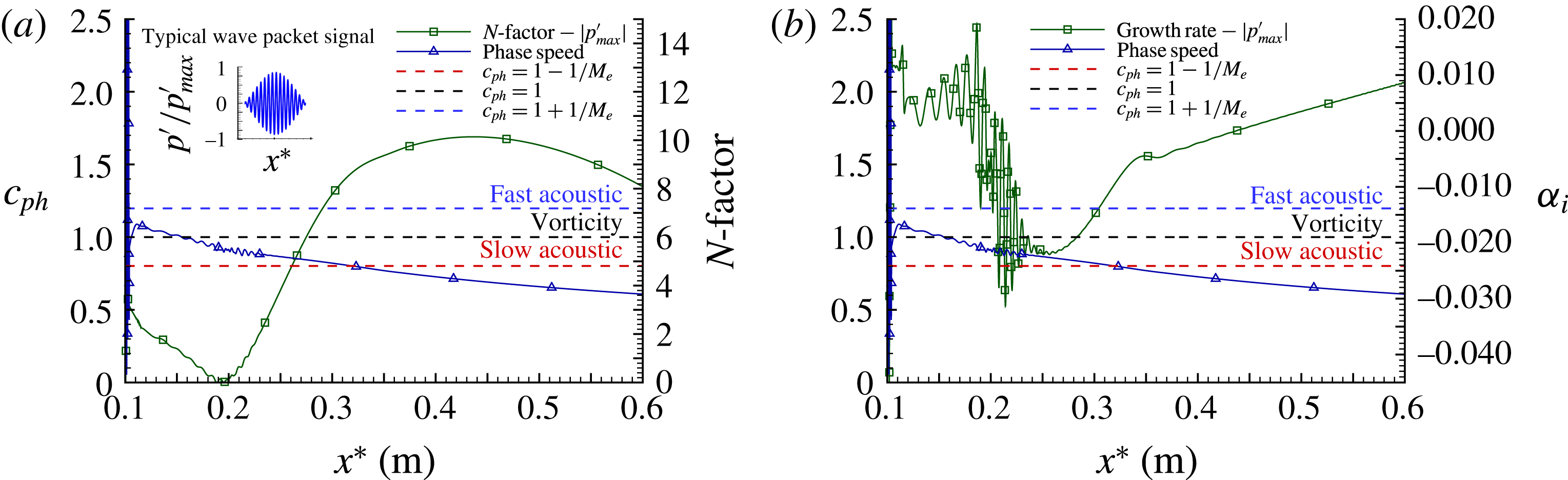
For the first case, the downstream propagation of a linear wave packet for axisymmetric disturbances was investigated. A typical instantaneous wave packet signal is shown in the inset of figure 1(a). From the DNS data, growth rates,
 $N$
-factors and phase speeds can be extracted for any wave component (i.e. Fourier mode) employing Fourier analysis. For example, in figure 1(a), the downstream development of the
 $N$
-factor and the phase speed for an amplified second-mode wave with
 $f^{\ast }=2.036$
MHz are shown. In addition, in figure 1(a), the phase speeds of the fast acoustic waves (i.e.
 $c_{ph}=1+1/M_{e}$
), the entropy/vorticity waves (i.e.
 $c_{ph}=1$
) and the slow acoustic (i.e.
 $c_{ph}=1-1/M_{e}$
) waves are shown as well. In figure 1(a), oscillations of the phase speed can be observed, which start slightly upstream of the synchronization location (i.e. where the phase speed of the second-mode wave crosses that of the vorticity/entropy waves). The oscillations become more pronounced as the phase speed of the second-mode wave decreases further, while crossing the lower neutral stability branch (i.e.
 $N=0$
). It should be noted that oscillations can also be observed in the
 $N$
-factor curve in approximately the same downstream region (approximately between
 $x^{\ast }=0.18~\text{m}$
and
 $x^{\ast }=0.22~\text{m}$
) and that the synchronization location is slightly upstream of the neutral point. These oscillations are much more pronounced for the amplification rates, which are plotted in figure 1(b) together with the phase speed. The largest oscillations of the wave speed occur at approximately
 $x^{\ast }=0.2~\text{m}$
, that is, at the same location where the wave changes from damped to amplified (i.e.
 $N=0$
in figure 1
a). The oscillations in both the
 $N$
-factor and the growth rate decay right after the phase speed crosses the neutral point. Moreover, the maximum growth rate is located downstream of this point. As shown in figure 1(a), an
 $N$
-factor of 9 is reached slightly before
 $x^{\ast }=0.35~\text{m}$
. Immediately downstream of this location, a slight ‘bump’ develops in the growth rate curve, after which an almost linear decrease with streamwise distance sets in. This decrease occurs after the phase speed of the wave has reached the phase speed of the slow acoustic wave. The same behaviour as discussed above was also observed for the other amplified second-mode frequency components resulting from the DNS of the linear axisymmetric wave packet, as well as for three-dimensional wave packets as discussed by Salemi et al. (Reference Salemi, Fasel, Wernz and Marquart2014).
Axisymmetric linear wave packet downstream development of phase speed and stability parameters for
 $f^{\ast }=2.036$
MHz: (a) phase speed and
 $N$
-factor, (b) phase speed and growth rate.

Salemi et al. (Reference Salemi, Fasel, Wernz and Marquart2014) presented evidence that for the T5 flow conditions, spatial oscillations of the wall-pressure signal are related to the synchronization of the second-mode waves with modes from the continuous spectrum. According to Mack (Reference Mack1984), when a region within the boundary layer exists in which a wave component becomes locally supersonic relative to the mean flow (i.e.
 $c_{ph}^{\ast }-U(y)^{\ast }>a_{e}^{\ast }$
), the wavenumber for such a wave is no longer unique and there is an infinite number of discrete neutral subsonic disturbances called ‘higher subsonic neutral modes’ if
 $U_{e}^{\ast }-a_{e}^{\ast }<c_{ph}^{\ast }<U_{e}^{\ast }$
and ‘regular neutral solutions’ if
 $U_{e}^{\ast }<c_{ph}^{\ast }<U_{e}^{\ast }+a_{e}^{\ast }$
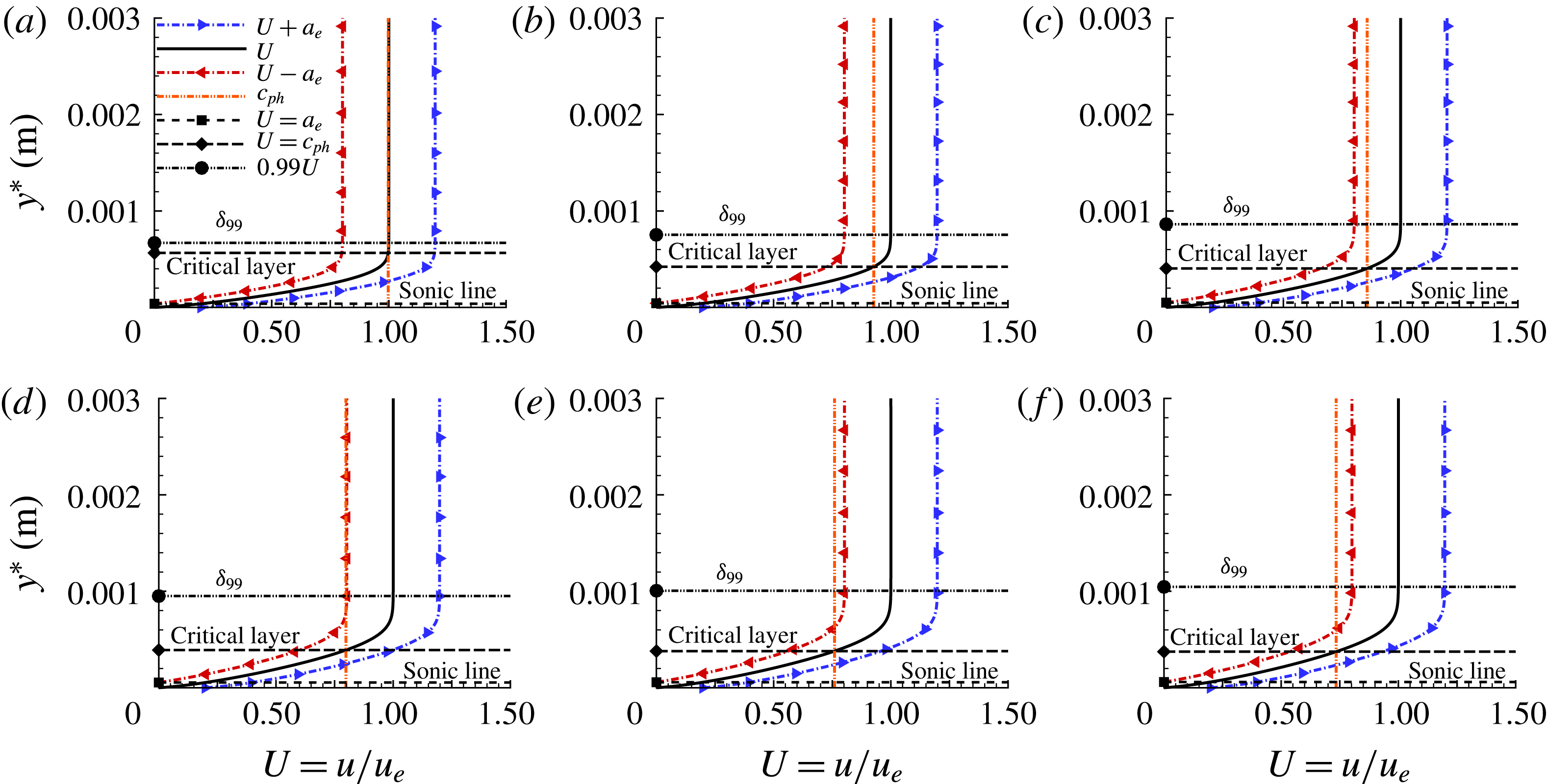
. The ‘higher subsonic neutral modes’ are related to the presence of the generalized inflection point whereas the ‘regular neutral solutions’ are not. It can be seen in figure 1 that, at first, the phase speed of the second-mode wave is between those of the fast acoustic and vorticity/entropy modes, which means that the instability is due to the existence of a region close to the wall in which the wave becomes supersonic in relation to the local flow velocity and therefore is not related to the existence of a generalized inflection point. It also means that at first this wave is a ‘regular solution’, and as it slows down in the downstream direction (figure 1), it becomes a ‘higher subsonic mode’. This situation is explained with the phase speed profiles shown in figure 2(a–f). The profiles in figure 2 were extracted at the locations marked in figure 3. At location 1, the phase speed coincides with the edge velocity (figure 2
a), where there is a large locally supersonic region (i.e.
 $c_{ph}^{\ast }-U(y)^{\ast }>a_{e}^{\ast }$
), which is necessary for the instability to exist (Mack Reference Mack1984). It should be noted that although the boundary layer grows downstream, the critical layer still moves towards the wall as the second-mode wave slows down. Past the synchronization point with the vorticity/entropy mode (location 2 in figure 3), the character of the solution changes to a ‘higher subsonic mode’ (figure 2
b). After crossing the first neutral branch, the phase speed approaches the sonic speed (figure 2
c) and the oscillations in the phase speed (figure 1) practically disappear (location 3 in figure 3). At the location where the wave becomes sonic (location 4 in figure 3), the wave speed lags in relation to the edge velocity by
 $a_{e}^{\ast }$
(figure 2
d) and an inflection point appears in the phase speed versus downstream direction (figure 1). At location 4 below the critical layer, the locally supersonic region (i.e.
 $c_{ph}^{\ast }-U(y)^{\ast }>a_{e}^{\ast }$
) is still present. Past this location, another locally supersonic region appears above the critical layer, in which
 $U_{e}^{\ast }-c_{ph}^{\ast }>a_{e}^{\ast }$
(figure 2
e,f), meaning that the wave becomes a supersonic mode.
Axisymmetric linear wave packet phase speed profiles of a second-mode wave component for
 $f^{\ast }=2.036$
MHz: (a)
 $x^{\ast }=0.1590~\text{m}$
, (b)
 $x^{\ast }=0.2035~\text{m}$
, (c)
 $x^{\ast }=0.2700~\text{m}$
, (d)
 $x^{\ast }=0.3300~\text{m}$
, (e)
 $x^{\ast }=0.3700~\text{m}$
, (f)
 $x^{\ast }=0.4000~\text{m}$
. The
 $x^{\ast }$
locations are indicated in figure 3.

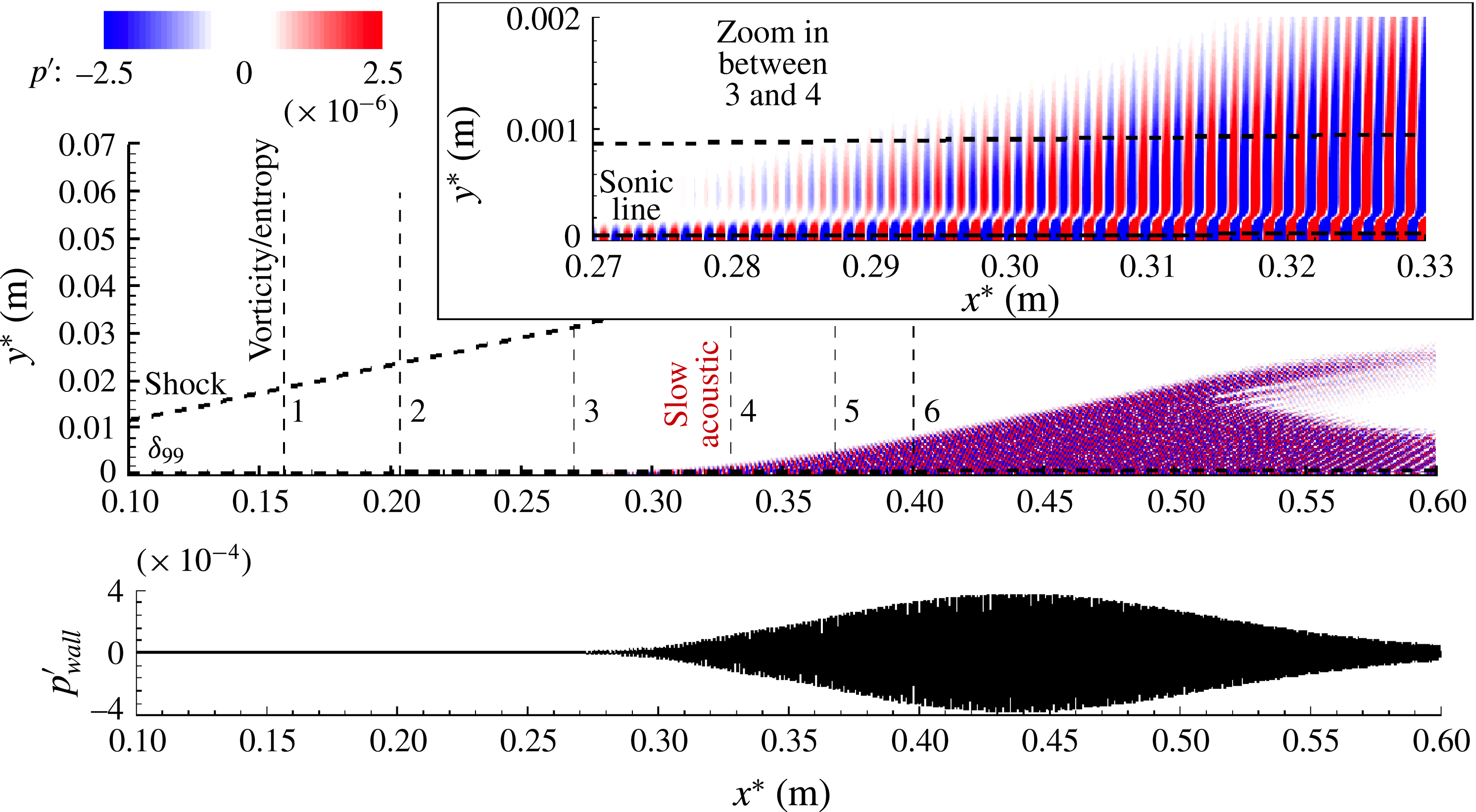
Overview of the axisymmetric linear wave train instantaneous pressure disturbance,
 $p^{\prime }$
, for
 $f^{\ast }=2036$
kHz,
 $A=10^{-6}$
. One can note also the synchronization locations with the vorticity/entropy and slow acoustic modes respectively.

4.2 Linear axisymmetric wave train – synchronization and acoustic emission
In order to extract more physical details regarding the synchronization mechanisms discussed above, a second DNS was performed with a continuous single-frequency forcing (using periodic wall blowing/suction through a slot). This forcing results in an axisymmetric wave train (in contrast to the wave packet as in § 4.1). For direct comparison with the observations discussed in § 4.1, a forcing frequency of
 $f^{\ast }=2.036$
MHz was used, for which the results were discussed in § 4.1 for the wave packet simulations. In figure 3, the instantaneous pressure disturbance field is shown, including the streamwise locations for which the various phase speed profiles were plotted in figure 2(a–f). A sudden emission of acoustic disturbances from inside the boundary layer into the free stream can be observed. The acoustic emission starts around the synchronization location with the slow acoustic wave (where the second-mode wave phase speed crosses that of the slow acoustic mode). One can note how deeply these waves penetrate into the inviscid flow region by comparing with the boundary layer thickness (
 $\unicode[STIX]{x1D6FF}_{99}$
is indicated in figure 3). Relative to the wall, the angle of the area contaminated by the acoustic emission is approximately
 $6.3^{\circ }$
, which is smaller than the angle of the Mach wave
 $(11.4^{\circ })$
.
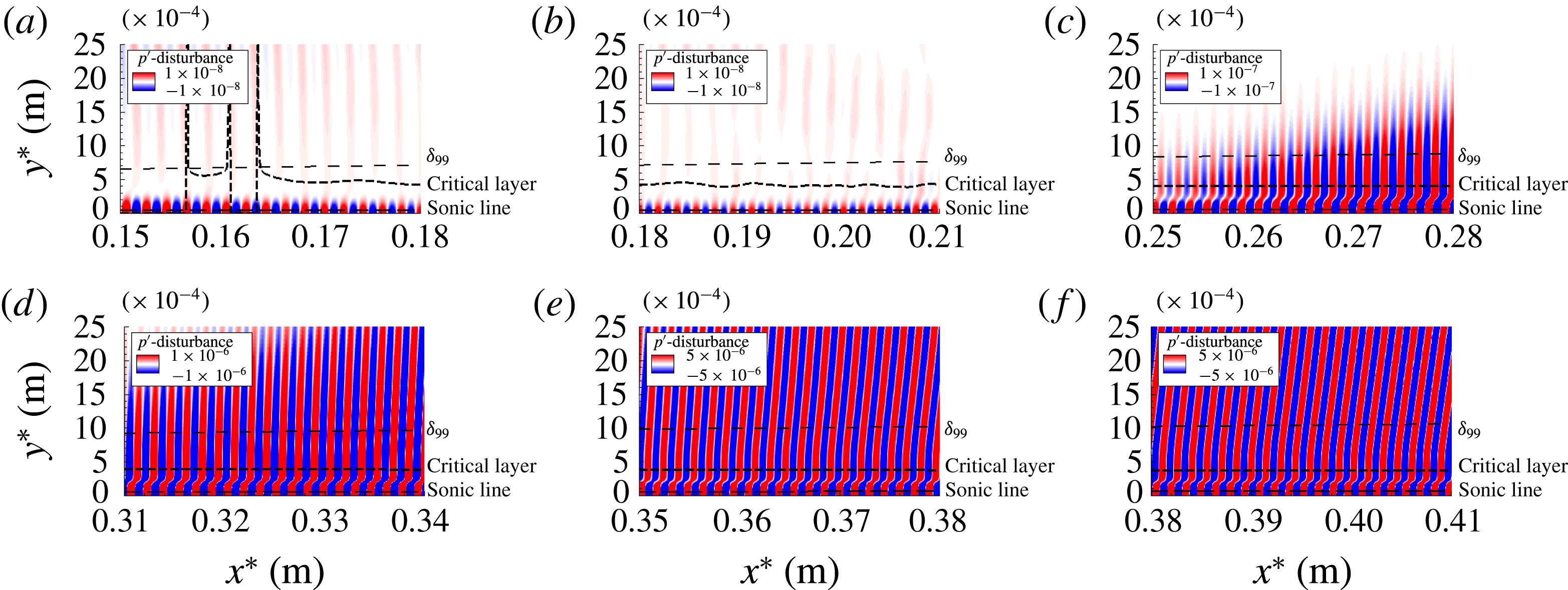
Detailed close-ups from figure 3. Instantaneous pressure disturbance,
 $p^{\prime }$
, for
 $f^{\ast }=2036~\text{kHz}$
,
 $A=10^{-6}$
at various streamwise regions: (a) region 1,
 $x^{\ast }=0.1590$
m; (b) region 2,
 $x^{\ast }=0.2035$
m; (c) region 3,
 $x^{\ast }=0.2700$
m; (d) region 4,
 $x^{\ast }=0.3300$
m; (e) region 5,
 $x^{\ast }=0.3700$
m; (f) region 6,
 $x^{\ast }=0.4000$
m.

Close-ups of the various regions of figure 3 reveal several details of the synchronization process and the emission of acoustic disturbances into the inviscid flow region. As can be observed in figure 4(a,b), the shock layer wave fronts that convect with the edge velocity connect (i.e. synchronize) with the second-mode waves near the wall. Moreover, as exhibited in figure 4(a), whenever these waves disconnect within the boundary layer, there is a discontinuity of the phase speed. Similar features can also be observed in figure 4(b). Figure 4(c) indicates that in the region slightly upstream of the synchronization location with the slow acoustic wave, the pressure disturbances start to penetrate into the inviscid flow field. At the synchronization location, an acoustic field is formed, which connects the second-mode waves to the inviscid shock layer (figure 4 d). At first, the wave fronts are nearly normal to the surface. Further downstream, the external acoustic field develops further and the wave fronts propagate at an angle (figure 4 e,f).
4.3 Nonlinear three-dimensional wave packet – acoustic emission
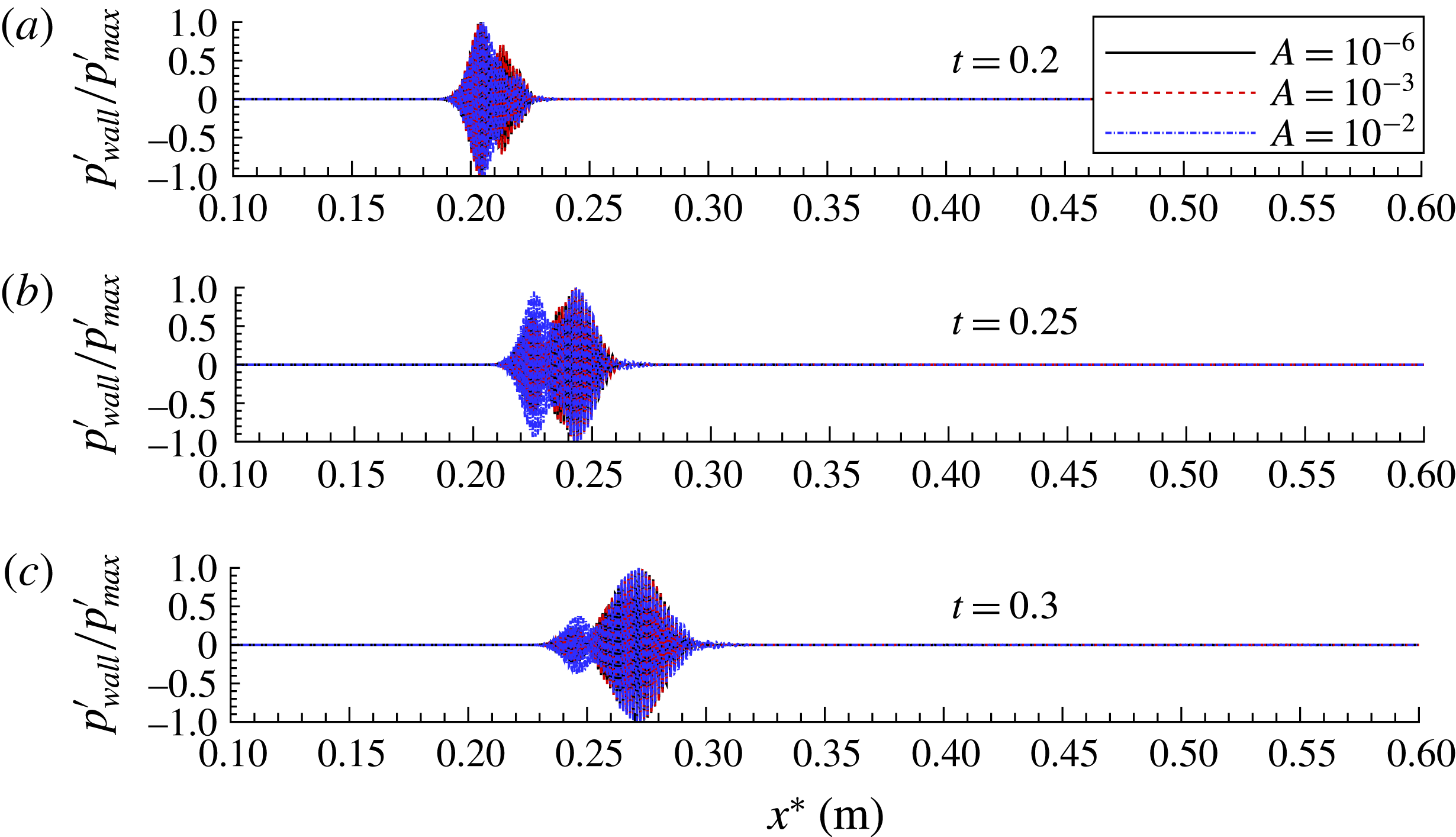
Instantaneous snapshots of a 3D wave packet for three pulse amplitudes:
 $A=10^{-6}$
(linear),
 $A=10^{-3}$
(weakly nonlinear) and
 $A=10^{-2}$
(strongly nonlinear). The normalized wall-pressure disturbances at the centreline of the packet are plotted versus the streamwise direction
 $x^{\ast }$
for
 $0.2\leqslant t\leqslant 0.3$
: (a)
 $t^{\ast }=49.019~\unicode[STIX]{x03BC}\text{s}$
, (b)
 $t^{\ast }=61.274~\unicode[STIX]{x03BC}\text{s}$
, (c)
 $t^{\ast }=73.529~\unicode[STIX]{x03BC}\text{s}$
.

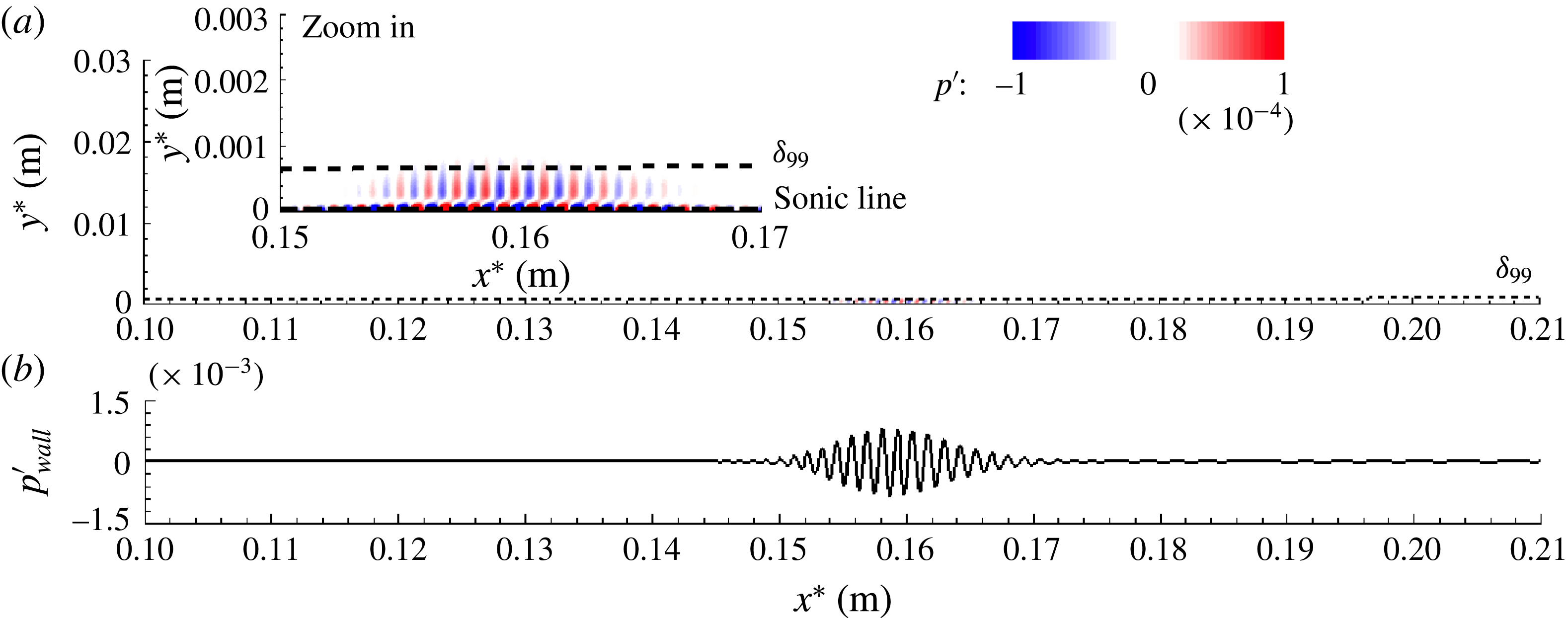
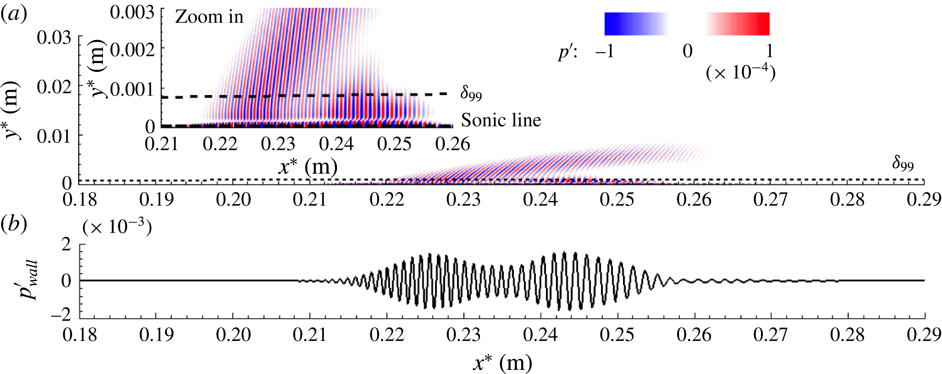
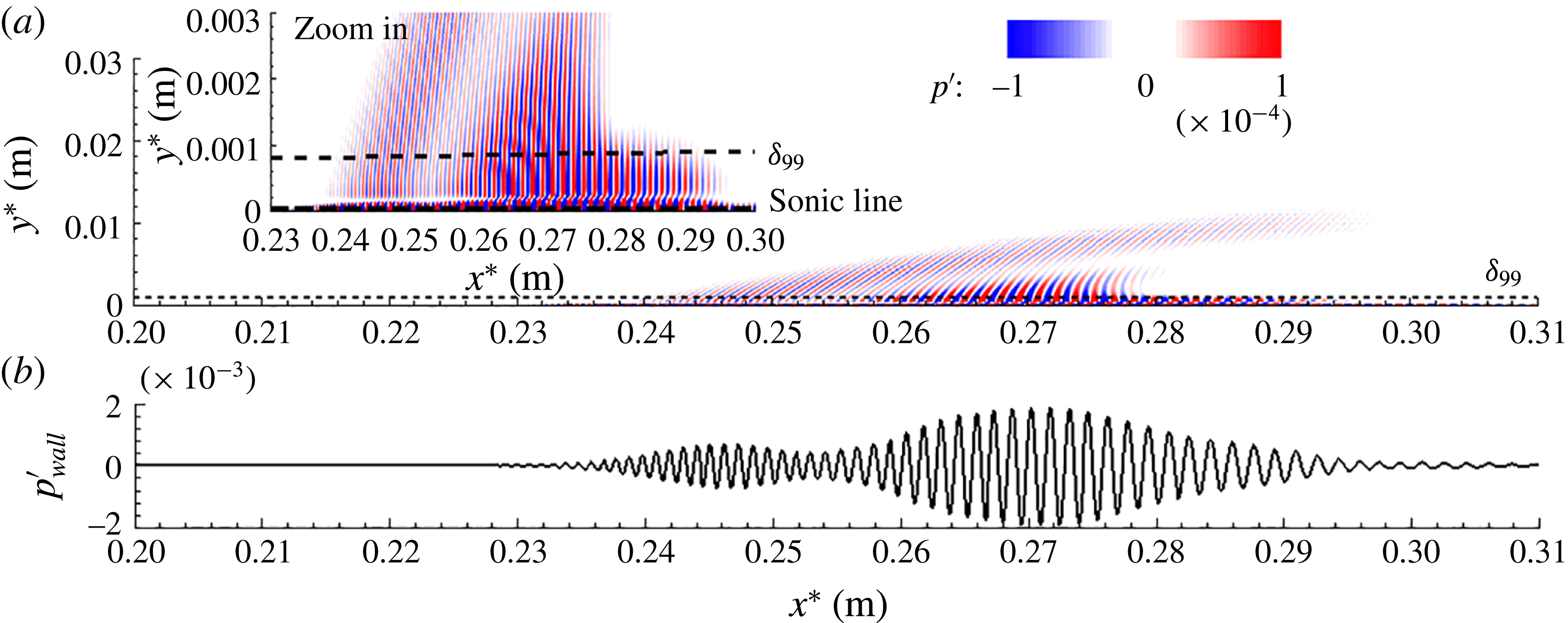
The phase speed synchronization of a second-mode wave component with continuous modes of the spectrum was demonstrated in § 4.1. In § 4.2, it was shown that synchronization with the slow acoustic mode results in the emission of acoustic disturbances deep into the free stream. In both cases, the disturbance amplitudes were assumed to be very small (i.e. negligible nonlinear effects) and the disturbances were axisymmetric. Now, the question arises of whether and how the observed phenomena are affected when the wave amplitudes are no longer small, so that nonlinear effects can occur, and when the waves can also be three-dimensional, as in realistic conditions of free flight or wind tunnel experiments. Towards answering this question, highly resolved DNS (with 438 million grid points) of three-dimensional wave packets were performed for several pulse amplitudes. In figure 5, the wall-pressure disturbances of the wave packets are displayed for several time instances and three different initial pulse amplitudes in order to better observe the nonlinear effects on the wave packet development. As can be seen in figure 5, the ‘linear’ (small-amplitude), ‘weakly nonlinear’ (intermediate-amplitude) and ‘strongly nonlinear’ (large-amplitude) wave packets all display qualitatively similar spatial modulations. Figure 6 clearly shows that in the region where the second-mode waves synchronize with the vorticity/entropy waves, the wave components in the middle of the packet (i.e. where the wall pressure
Nonlinear 3D wave packet,
 $A=10^{-2}$
: instantaneous pressure disturbance,
 $p^{\prime }$
, for time instant
 $t^{\ast }=24.509~\unicode[STIX]{x03BC}\text{s}$
when the wave packet has just passed the synchronization location with vorticity/entropy waves (see figure 1
a).

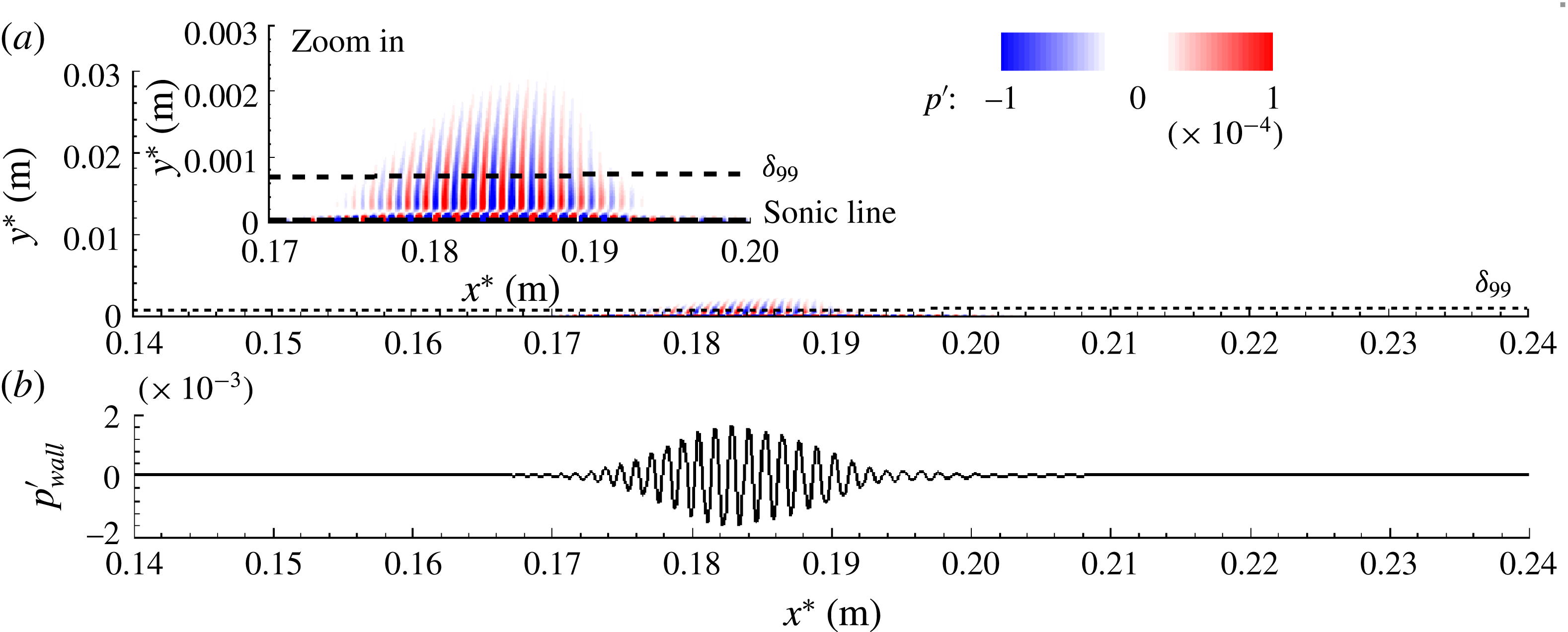
Nonlinear 3D wave packet,
 $A=10^{-2}$
: instantaneous pressure disturbance,
 $p^{\prime }$
, for time instant
 $t^{\ast }=36.764~\unicode[STIX]{x03BC}\text{s}$
when the wave packet is further downstream of the vorticity/entropy synchronization point. One can note the onset of acoustic emission as the first second-mode wave components of the packet cross the slow acoustic synchronization location.

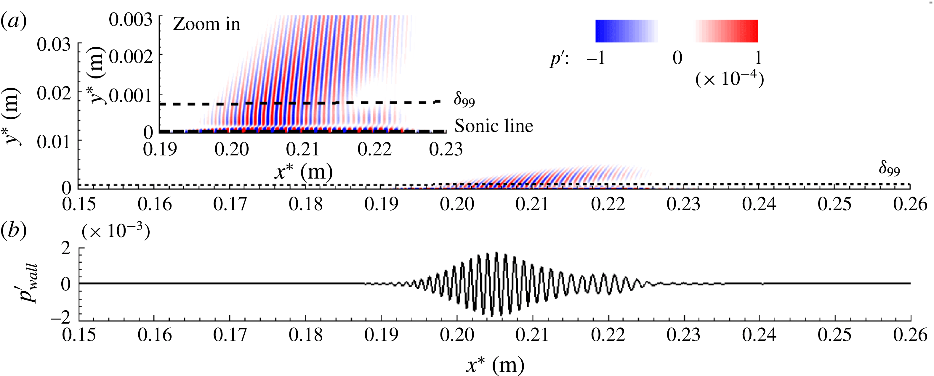
Nonlinear 3D wave packet,
 $A=10^{-2}$
: instantaneous pressure disturbance,
 $p^{\prime }$
, for time instant
 $t^{\ast }=49.019~\unicode[STIX]{x03BC}\text{s}$
. One can note the increased acoustic emission compared with figure 7 as more wave components cross the slow acoustic synchronization location.

Nonlinear 3D wave packet,
 $A=10^{-2}$
: instantaneous pressure disturbance,
 $p^{\prime }$
, for time instant
 $t^{\ast }=61.274~\unicode[STIX]{x03BC}\text{s}$
. One can note the increased acoustic emission compared with figure 8 as even more wave components of the packet cross the slow acoustic synchronization location.

has the largest amplitude) start to create a connection to the inviscid shock layer at the edge of the boundary layer. At this location, no spatial modulations in the wave packet signal are visible (figure 6
b). As the packet propagates closer to the lower neutral branch (figure 1
a), a connection to the inviscid free stream has been established, and the first signs of a spatial modulation can be noticed in the leading edge region of the wave packet (figure 7
b). As the second-mode wave components start to cross the lower neutral branch (figure 1
a), stronger spatial modulations of the packet start to develop in the leading edge of the packet (figure 8
b). It should be noted that for this location, acoustic disturbances are already ejected into the free stream. This can be explained by the fact that a wave packet consists of a broad range of frequencies and thus contains wave components with phase speeds lower than that of the wave with frequency
 $f^{\ast }=2036$
kHz that was considered in §§ 4.1 and 4.2. Therefore, the higher-frequency components of the packet reach the synchronization point with the slow acoustic wave earlier upstream than the lower frequencies. Moreover, it can be observed that the wave packet gets ‘stretched’ in the streamwise direction. For a location further downstream (figure 9), the spatial modulation becomes much more pronounced, with a broad reduction of amplitudes in the centre of the packet, which appears to be directly correlated with the acoustic emission. Finally, for a location further downstream, in figure 10, for which the majority of the second-mode wave components start to cross the synchronization location with the slow acoustic mode, the acoustic emission ‘covers’ almost the entire downstream extent of the packet. The strong modulation of the packet and the associated broad reduction of amplitudes (as seen in figures 8–10) appear to be directly correlated with the acoustic emission. This may be explained by the fact that the energy ejected into the free stream by these acoustic disturbances causes a reduction of kinetic energy of the second-mode instabilities remaining within the wave packet inside the boundary layer. Consequently, the acoustic emission causes a reduction of the disturbance amplitudes of the packet at the wall.
Nonlinear 3D wave packet,
 $A=10^{-2}$
: instantaneous pressure disturbance,
 $p^{\prime }$
, for time instant
 $t^{\ast }=73.529~\unicode[STIX]{x03BC}\text{s}$
. One can note the increased acoustic emission compared with figure 9.

5 Conclusions
Stability and transition of the Caltech T5 high-enthalpy boundary layer flow for a
 $5^{\circ }$
half-angle cone were investigated employing DNS. Wave packets and wave trains were simulated in the linear, weakly and strongly nonlinear regimes for both axisymmetric and 3D disturbance waves. It was found that the wave packets undergo spatial modulations that are caused by the synchronization between second-mode wave components and the vorticity/entropy modes. Furthermore, the synchronization with slow acoustic waves results in a sudden emission of acoustic waves deep into the free stream. The simulations revealed that the highly cooled wall (i.e.
 $T_{w}/T_{r}=0.04$
) of the Caltech T5 case leads to second-mode wave components, which become supersonic once synchronized with the slow acoustic continuous modes. The results for simulations of 3D larger-amplitude (nonlinear) wave packets demonstrated that these (linear) synchronization mechanisms, and also the sudden and strong emission of acoustic disturbances deep into the free stream, are not suppressed by nonlinear effects.
Acknowledgements
Parts of this work were funded by the AFOSR/NASA National Center of Hypersonic Laminar–Turbulent Transition Research at the Texas A&M University under grant FA9550-08-1-0211, with Dr J. Schmisseur serving as program manager, and by the Air Force Office of Scientific Research (AFOSR) under grant FA9550-15-1-0265, with Dr I. Leyva serving as program manager. The authors thank Drs J. Jewell, J. Shepherd and H. Hornung for fruitful discussions.
Appendix A
The vectors in the conservation equations (2.3) are defined as
 $$\begin{eqnarray}\boldsymbol{E}_{\boldsymbol{C}}=\left[\begin{array}{@{}c@{}}\unicode[STIX]{x1D70C}u\\ \unicode[STIX]{x1D70C}u^{2}+p\\ \unicode[STIX]{x1D70C}uv\\ \unicode[STIX]{x1D70C}uw\\ (\unicode[STIX]{x1D70C}E_{t}+p)u\end{array}\right]\!,\quad \boldsymbol{F}_{\boldsymbol{C}}=\left[\begin{array}{@{}c@{}}\unicode[STIX]{x1D70C}v\\ \unicode[STIX]{x1D70C}uv\\ \unicode[STIX]{x1D70C}v^{2}+p\\ \unicode[STIX]{x1D70C}vw\\ (\unicode[STIX]{x1D70C}E_{t}+p)v\end{array}\right]\!,\quad \boldsymbol{G}_{\boldsymbol{C}}=\left[\begin{array}{@{}c@{}}\unicode[STIX]{x1D70C}w\\ \unicode[STIX]{x1D70C}uw\\ \unicode[STIX]{x1D70C}vw\\ \unicode[STIX]{x1D70C}w^{2}+p\\ (\unicode[STIX]{x1D70C}E_{t}+p)w\end{array}\right]\!,\end{eqnarray}$$
 $$\begin{eqnarray}\boldsymbol{E}_{\boldsymbol{D}}=\left[\begin{array}{@{}c@{}}0\\ -\unicode[STIX]{x1D70F}_{xx}\\ -\unicode[STIX]{x1D70F}_{xy}\\ -\unicode[STIX]{x1D70F}_{x\unicode[STIX]{x1D719}}\\ q_{x}+(-u\unicode[STIX]{x1D70F}_{xx}-v\unicode[STIX]{x1D70F}_{xy}-w\unicode[STIX]{x1D70F}_{x\unicode[STIX]{x1D719}})\end{array}\right]\!,\quad \boldsymbol{F}_{\boldsymbol{D}}=\left[\begin{array}{@{}c@{}}0\\ -\unicode[STIX]{x1D70F}_{xy}\\ -\unicode[STIX]{x1D70F}_{yy}\\ -\unicode[STIX]{x1D70F}_{y\unicode[STIX]{x1D719}}\\ q_{y}+(-u\unicode[STIX]{x1D70F}_{xy}-v\unicode[STIX]{x1D70F}_{yy}-w\unicode[STIX]{x1D70F}_{y\unicode[STIX]{x1D719}})\end{array}\right]\!,\end{eqnarray}$$
 $$\begin{eqnarray}\boldsymbol{G}_{\boldsymbol{D}}=\left[\begin{array}{@{}c@{}}0\\ -\unicode[STIX]{x1D70F}_{x\unicode[STIX]{x1D719}}\\ -\unicode[STIX]{x1D70F}_{y\unicode[STIX]{x1D719}}\\ -\unicode[STIX]{x1D70F}_{\unicode[STIX]{x1D719}\unicode[STIX]{x1D719}}\\ q_{\unicode[STIX]{x1D719}}+(-u\unicode[STIX]{x1D70F}_{x\unicode[STIX]{x1D719}}-v\unicode[STIX]{x1D70F}_{y\unicode[STIX]{x1D719}}-w\unicode[STIX]{x1D70F}_{\unicode[STIX]{x1D719}\unicode[STIX]{x1D719}})\end{array}\right]\!,\quad \!\boldsymbol{H}=\frac{1}{r}\!\left[\begin{array}{@{}c@{}}0\\ -\text{sin}\,\unicode[STIX]{x1D703}_{c}(\unicode[STIX]{x1D70C}w^{2}-\unicode[STIX]{x1D70F}_{\unicode[STIX]{x1D719}\unicode[STIX]{x1D719}}+p)\\ -\text{cos}\,\unicode[STIX]{x1D703}_{c}(\unicode[STIX]{x1D70C}w^{2}-\unicode[STIX]{x1D70F}_{\unicode[STIX]{x1D719}\unicode[STIX]{x1D719}}+p)\\ \sin \unicode[STIX]{x1D703}_{c}(\unicode[STIX]{x1D70C}uw-\unicode[STIX]{x1D70F}_{x\unicode[STIX]{x1D719}})+\cos \unicode[STIX]{x1D703}_{c}(\unicode[STIX]{x1D70C}vw-\unicode[STIX]{x1D70F}_{y\unicode[STIX]{x1D719}})\\ 0\end{array}\right]\!,\end{eqnarray}$$
where
 $\boldsymbol{E}_{\boldsymbol{C}}$
,
 $\boldsymbol{F}_{\boldsymbol{C}}$
and
 $\boldsymbol{G}_{\boldsymbol{C}}$
are the convective fluxes in the streamwise, normal and azimuthal directions respectively. Accordingly,
 $\boldsymbol{E}_{\boldsymbol{D}}$
,
 $\boldsymbol{F}_{\boldsymbol{D}}$
and
 $\boldsymbol{G}_{\boldsymbol{D}}$
are the diffusive fluxes in the streamwise, normal and azimuthal directions, and
 $\boldsymbol{H}$
is the source term.
The stresses are defined as
 $$\begin{eqnarray}\displaystyle & \displaystyle \unicode[STIX]{x1D70F}_{xx}=\frac{\unicode[STIX]{x1D707}}{Re}\left[\frac{4}{3}\frac{\unicode[STIX]{x2202}u}{\unicode[STIX]{x2202}x}-\frac{2}{3}\frac{\unicode[STIX]{x2202}v}{\unicode[STIX]{x2202}y}-\frac{2}{3}\frac{1}{r}\frac{\unicode[STIX]{x2202}w}{\unicode[STIX]{x2202}\unicode[STIX]{x1D719}}-\frac{2}{3}\frac{1}{r}(u\sin \unicode[STIX]{x1D703}_{c}+v\cos \unicode[STIX]{x1D703}_{c})\right]\!,\qquad \;\quad & \displaystyle\end{eqnarray}$$
 $$\begin{eqnarray}\displaystyle & \displaystyle \unicode[STIX]{x1D70F}_{yy}=\frac{\unicode[STIX]{x1D707}}{Re}\left[\frac{4}{3}\frac{\unicode[STIX]{x2202}v}{\unicode[STIX]{x2202}y}-\frac{2}{3}\frac{\unicode[STIX]{x2202}u}{\unicode[STIX]{x2202}x}-\frac{2}{3}\frac{1}{r}\frac{\unicode[STIX]{x2202}w}{\unicode[STIX]{x2202}\unicode[STIX]{x1D719}}-\frac{2}{3}\frac{1}{r}(u\sin \unicode[STIX]{x1D703}_{c}+v\cos \unicode[STIX]{x1D703}_{c})\right]\!,\qquad \;\quad & \displaystyle\end{eqnarray}$$
 $$\begin{eqnarray}\displaystyle & \displaystyle \unicode[STIX]{x1D70F}_{\unicode[STIX]{x1D719}\unicode[STIX]{x1D719}}=\frac{\unicode[STIX]{x1D707}}{Re}\left[\frac{4}{3}\frac{1}{r}\frac{\unicode[STIX]{x2202}w}{\unicode[STIX]{x2202}\unicode[STIX]{x1D719}}-\frac{2}{3}\frac{\unicode[STIX]{x2202}u}{\unicode[STIX]{x2202}x}-\frac{2}{3}\frac{\unicode[STIX]{x2202}v}{\unicode[STIX]{x2202}y}+\frac{4}{3}\frac{1}{r}(u\sin \unicode[STIX]{x1D703}_{c}+v\cos \unicode[STIX]{x1D703}_{c})\right]\!,\qquad \;\quad & \displaystyle\end{eqnarray}$$
 $$\begin{eqnarray}\unicode[STIX]{x1D70F}_{xy}=\frac{\unicode[STIX]{x1D707}}{Re}\left(\frac{\unicode[STIX]{x2202}v}{\unicode[STIX]{x2202}x}+\frac{\unicode[STIX]{x2202}u}{\unicode[STIX]{x2202}y}\right),\quad \unicode[STIX]{x1D70F}_{x\unicode[STIX]{x1D719}}=\frac{\unicode[STIX]{x1D707}}{Re}\left(\frac{1}{r}\frac{\unicode[STIX]{x2202}u}{\unicode[STIX]{x2202}\unicode[STIX]{x1D719}}+\frac{\unicode[STIX]{x2202}w}{\unicode[STIX]{x2202}x}-\frac{1}{r}w\sin \unicode[STIX]{x1D703}_{c}\right)\!,\end{eqnarray}$$
 $$\begin{eqnarray}\unicode[STIX]{x1D70F}_{y\unicode[STIX]{x1D719}}=\frac{\unicode[STIX]{x1D707}}{Re}\left(\frac{1}{r}\frac{\unicode[STIX]{x2202}v}{\unicode[STIX]{x2202}\unicode[STIX]{x1D719}}+\frac{\unicode[STIX]{x2202}w}{\unicode[STIX]{x2202}y}-\frac{1}{r}w\cos \unicode[STIX]{x1D703}_{c}\right)\!.\qquad \quad\end{eqnarray}$$
The components of the heat-flux vector in each direction (i.e.
 $x$
,
 $y$
and
 $\unicode[STIX]{x1D719}$
) are
 $$\begin{eqnarray}q_{x}=-\frac{\unicode[STIX]{x1D707}}{(\unicode[STIX]{x1D6FE}-1)M^{2}\,Re\,Pr}\frac{\unicode[STIX]{x2202}T}{\unicode[STIX]{x2202}x},\quad q_{y}=-\frac{\unicode[STIX]{x1D707}}{(\unicode[STIX]{x1D6FE}-1)M^{2}\,Re\,Pr}\frac{\unicode[STIX]{x2202}T}{\unicode[STIX]{x2202}y},\end{eqnarray}$$
 $$\begin{eqnarray}q_{\unicode[STIX]{x1D719}}=-\frac{\unicode[STIX]{x1D707}}{(\unicode[STIX]{x1D6FE}-1)M^{2}\,Re\,Pr}\frac{1}{r}\frac{\unicode[STIX]{x2202}T}{\unicode[STIX]{x2202}\unicode[STIX]{x1D719}},\end{eqnarray}$$
where
 $Re$
,
 $Pr$
and
 $M$
are the Reynolds number, Prandtl number and Mach number respectively, and are defined herein as
 $$\begin{eqnarray}Re=\frac{\unicode[STIX]{x1D70C}_{\infty }^{\ast }\,U_{\infty }^{\ast }\,L^{\ast }}{\unicode[STIX]{x1D707}_{\infty }^{\ast }},\quad Pr=\frac{\unicode[STIX]{x1D707}_{\infty }^{\ast }\,{c_{p\infty }}^{\ast }}{\unicode[STIX]{x1D705}_{\infty }^{\ast }},\quad M=\frac{U_{\infty }^{\ast }}{\sqrt{\unicode[STIX]{x1D6FE}p_{\infty }^{\ast }/\unicode[STIX]{x1D70C}_{\infty }^{\ast }}}.\end{eqnarray}$$
The gas state equation provides closure for the system of conservation equations and is given by
 $$\begin{eqnarray}p=\frac{\unicode[STIX]{x1D70C}\,T}{\unicode[STIX]{x1D6FE}M^{2}}.\end{eqnarray}$$