



%20--%3e%3c!DOCTYPE%20svg%20PUBLIC%20'-//W3C//DTD%20SVG%201.0//EN'%20'http://www.w3.org/TR/2001/REC-SVG-20010904/DTD/svg10.dtd'%3e%3csvg%20version='1.0'%20id='Layer_1'%20xmlns='http://www.w3.org/2000/svg'%20xmlns:xlink='http://www.w3.org/1999/xlink'%20x='0px'%20y='0px'%20width='64px'%20height='64px'%20viewBox='5.5%20-3.5%2064%2064'%20enable-background='new%205.5%20-3.5%2064%2064'%20xml:space='preserve'%3e%3cg%3e%3ccircle%20fill='%23FFFFFF'%20fill-opacity='0'%20cx='37.785'%20cy='28.501'%20r='28.836'/%3e%3cpath%20fill='%23595959'%20d='M37.441-3.5c8.951,0,16.572,3.125,22.857,9.372c3.008,3.009,5.295,6.448,6.857,10.314%20c1.561,3.867,2.344,7.971,2.344,12.314c0,4.381-0.773,8.486-2.314,12.313c-1.543,3.828-3.82,7.21-6.828,10.143%20c-3.123,3.085-6.666,5.448-10.629,7.086c-3.961,1.638-8.057,2.457-12.285,2.457s-8.276-0.808-12.143-2.429%20c-3.866-1.618-7.333-3.961-10.4-7.027c-3.067-3.066-5.4-6.524-7-10.372S5.5,32.767,5.5,28.5c0-4.229,0.809-8.295,2.428-12.2%20c1.619-3.905,3.972-7.4,7.057-10.486C21.08-0.394,28.565-3.5,37.441-3.5z%20M37.557,2.272c-7.314,0-13.467,2.553-18.458,7.657%20c-2.515,2.553-4.448,5.419-5.8,8.6c-1.354,3.181-2.029,6.505-2.029,9.972c0,3.429,0.675,6.734,2.029,9.913%20c1.353,3.183,3.285,6.021,5.8,8.516c2.514,2.496,5.351,4.399,8.515,5.715c3.161,1.314,6.476,1.971,9.943,1.971%20c3.428,0,6.75-0.665,9.973-1.999c3.219-1.335,6.121-3.257,8.713-5.771c4.99-4.876,7.484-10.99,7.484-18.344%20c0-3.543-0.648-6.895-1.943-10.057c-1.293-3.162-3.18-5.98-5.654-8.458C50.984,4.844,44.795,2.272,37.557,2.272z%20M37.156,23.187%20l-4.287,2.229c-0.458-0.951-1.019-1.619-1.685-2c-0.667-0.38-1.286-0.571-1.858-0.571c-2.856,0-4.286,1.885-4.286,5.657%20c0,1.714,0.362,3.084,1.085,4.113c0.724,1.029,1.791,1.544,3.201,1.544c1.867,0,3.181-0.915,3.944-2.743l3.942,2%20c-0.838,1.563-2,2.791-3.486,3.686c-1.484,0.896-3.123,1.343-4.914,1.343c-2.857,0-5.163-0.875-6.915-2.629%20c-1.752-1.752-2.628-4.19-2.628-7.313c0-3.048,0.886-5.466,2.657-7.257c1.771-1.79,4.009-2.686,6.715-2.686%20C32.604,18.558,35.441,20.101,37.156,23.187z%20M55.613,23.187l-4.229,2.229c-0.457-0.951-1.02-1.619-1.686-2%20c-0.668-0.38-1.307-0.571-1.914-0.571c-2.857,0-4.287,1.885-4.287,5.657c0,1.714,0.363,3.084,1.086,4.113%20c0.723,1.029,1.789,1.544,3.201,1.544c1.865,0,3.18-0.915,3.941-2.743l4,2c-0.875,1.563-2.057,2.791-3.541,3.686%20c-1.486,0.896-3.105,1.343-4.857,1.343c-2.896,0-5.209-0.875-6.941-2.629c-1.736-1.752-2.602-4.19-2.602-7.313%20c0-3.048,0.885-5.466,2.658-7.257c1.77-1.79,4.008-2.686,6.713-2.686C51.117,18.558,53.938,20.101,55.613,23.187z'/%3e%3c/g%3e%3c/svg%3e)
%20--%3e%3c!DOCTYPE%20svg%20PUBLIC%20'-//W3C//DTD%20SVG%201.0//EN'%20'http://www.w3.org/TR/2001/REC-SVG-20010904/DTD/svg10.dtd'%3e%3csvg%20version='1.0'%20id='Layer_1'%20xmlns='http://www.w3.org/2000/svg'%20xmlns:xlink='http://www.w3.org/1999/xlink'%20x='0px'%20y='0px'%20width='64px'%20height='64px'%20viewBox='5.5%20-3.5%2064%2064'%20enable-background='new%205.5%20-3.5%2064%2064'%20xml:space='preserve'%3e%3cg%3e%3ccircle%20fill='%23FFFFFF'%20fill-opacity='0'%20cx='37.637'%20cy='28.806'%20r='28.276'/%3e%3cg%3e%3cpath%20fill='%23595959'%20d='M37.443-3.5c8.988,0,16.57,3.085,22.742,9.257C66.393,11.967,69.5,19.548,69.5,28.5c0,8.991-3.049,16.476-9.145,22.456%20C53.879,57.319,46.242,60.5,37.443,60.5c-8.649,0-16.153-3.144-22.514-9.43C8.644,44.784,5.5,37.262,5.5,28.5%20c0-8.761,3.144-16.342,9.429-22.742C21.101-0.415,28.604-3.5,37.443-3.5z%20M37.557,2.272c-7.276,0-13.428,2.553-18.457,7.657%20c-5.22,5.334-7.829,11.525-7.829,18.572c0,7.086,2.59,13.22,7.77,18.398c5.181,5.182,11.352,7.771,18.514,7.771%20c7.123,0,13.334-2.607,18.629-7.828c5.029-4.838,7.543-10.952,7.543-18.343c0-7.276-2.553-13.465-7.656-18.571%20C50.967,4.824,44.795,2.272,37.557,2.272z%20M46.129,20.557v13.085h-3.656v15.542h-9.944V33.643h-3.656V20.557%20c0-0.572,0.2-1.057,0.599-1.457c0.401-0.399,0.887-0.6,1.457-0.6h13.144c0.533,0,1.01,0.2,1.428,0.6%20C45.918,19.5,46.129,19.986,46.129,20.557z%20M33.042,12.329c0-3.008,1.485-4.514,4.458-4.514s4.457,1.504,4.457,4.514%20c0,2.971-1.486,4.457-4.457,4.457S33.042,15.3,33.042,12.329z'/%3e%3c/g%3e%3c/g%3e%3c/svg%3e)
1. Introduction
The intermittency of wind and solar energy is a great challenge facing the current transition away from fossil fuels (Wallace et al. Reference Wallace, Cai, Zhang, Zhang and Guo2021). Even with an enormous wind and solar network, without energy storage, 20 % of the total energy demand could go unmet (Delarue & Morris Reference Delarue and Morris2015). One promising solution is the large-scale storage of hydrogen in underground porous layers, which have a surplus capacity relative to current requirements (Carden & Paterson Reference Carden and Paterson1979; Luboń & Tarkowski Reference Luboń and Tarkowski2020; Ennis-King et al. Reference Ennis-King, Michael, Strand, Sander and Green2021).
At times of high renewable output and relatively low demand, electricity is used to generate hydrogen, which is injected directly in subsurface porous layers that are bounded above by an impermeable seal rock. Subsequently, the hydrogen is withdrawn to meet demand. Efficient underground storage of hydrogen is challenging due to a combination of interdependent processes that are not fully understood. For example, the very low density and viscosity of hydrogen relative to the ambient water can trigger flow instabilities (Heinemann et al. Reference Heinemann, Alcalde, Miocic, Hangx, Kallmeyer, Ostertag-Henning, Hassanpouryouzband, Thaysen, Strobel and Schmidt-Hattenberger2021), subsurface microbes may consume hydrogen and clog the pore space (Thaysen et al. Reference Thaysen, McMahon, Strobel, Butler, Ngwenya, Heinemann, Wilkinson, Hassanpouryouzband, McDermott and Edlmann2021), and, over long time scales, there may be a nonlinear interaction between injection-driven flows followed by withdrawal-driven flows (Dudfield & Woods Reference Dudfield and Woods2012; Krevor et al. Reference Krevor, De Coninck, Gasda, Ghaleigh, de Gooyert, Hajibeygi, Juanes, Neufeld, Roberts and Swennenhuis2023).
In the present study, we analyse the effect of microbial growth on the buoyancy-driven flow of hydrogen that is injected into a porous layer. The microbes grow within biofilms on the porous rock, supplied by the invading hydrogen, and this reduces the porosity and permeability of the layer. The zone where hydrogen has been resident longest has the lowest porosity. The resulting transient heterogeneity within the porous rock leads to rich flow structures, as has been observed for pressure-driven flows with precipitation reactions (Nagatsu et al. Reference Nagatsu, Ishii, Tada and De Wit2014; Sabet, Hassanzadeh & Abedi Reference Sabet, Hassanzadeh and Abedi2020).
One of the central concerns in subsurface hydrogen storage is understanding fluid migration, which has a significant impact on operational performance (Wang et al. Reference Wang, Pickup, Sorbie and Mackay2022). This paper focuses on how the combination of buoyancy forces, microbial consumption of hydrogen and microbe-induced alteration of the rock properties influences hydrogen flow. Whilst there is still some uncertainty in the rates of these processes, we are interested in providing general insights into the flow physics, the interplay of the different physical and biological ingredients in the model, and the dependencies on kinetic and subsurface parameters.
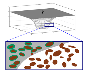
Given the two key ingredients to the model (buoyancy-driven flow and microbial activity; see figure 1), we break this section into two parts. First, a brief review of buoyancy-driven flow in a porous layer is given in § 1.1 and then in § 1.2, we discuss microbial growth and its effect on porosity, permeability and hydrogen consumption.
(a) Schematic of the buoyancy-driven flow of hydrogen with input flux  $Q_{in}$ into a porous layer bounded above by a horizontal impermeable seal. The porosity reduces in proportion to the hydrogen residence time owing to biofilm growth on the porous rock. (b) Radial cross-section of the axisymmetric flow. (c) Schematic of the pore-scale features.

1.1. Porous gravity currents
The shape of the fluid envelope resulting from the input of a relatively buoyant fluid into a porous medium bounded above by an impermeable layer is initially hemispherical because injection dominates (Huppert & Pegler Reference Huppert and Pegler2022). However, at later times, the pressure gradient associated with injection becomes small relative to gradients of the hydrostatic pressure (Nordbotten & Celia Reference Nordbotten and Celia2006; Huppert & Pegler Reference Huppert and Pegler2022; Zheng Reference Zheng2023). Subsequently, the flow is predominantly radial, driven by radial gradients of the hydrostatic pressure, and the layer of input fluid becomes relatively thin ( $\text {thickness}/\text {radial extent}\ll 1$; see figure 1a) (Bear Reference Bear1988; Huppert & Woods Reference Huppert and Woods1995).
This analysis has been validated experimentally (Lyle et al. Reference Lyle, Huppert, Hallworth, Bickle and Chadwick2005; Huppert & Pegler Reference Huppert and Pegler2022) and through numerical simulations (Hagemann et al. Reference Hagemann, Rasoulzadeh, Panfilov, Ganzer and Reitenbach2015). Such a flow configuration is known as a ‘porous gravity current’ and the transition time to this behaviour is given by (2.2).
Porous gravity currents have been widely studied owing to their relatively simple mathematical treatment and the accuracy with which they capture observations from the laboratory and the subsurface (Lyle et al. Reference Lyle, Huppert, Hallworth, Bickle and Chadwick2005; Bickle et al. Reference Bickle, Chadwick, Huppert, Hallworth and Lyle2007; Pegler, Huppert & Neufeld Reference Pegler, Huppert and Neufeld2014). The gravity current model has been adapted to study a wide range of physical phenomena that arise in subsurface flows, often motivated by engineering challenges associated with  ${\rm CO}_{2}$ sequestration. Examples include the influence of confinement on the flow, whereby the displacement of the ambient fluid plays a key role in the motion (Pegler et al. Reference Pegler, Huppert and Neufeld2014; Zheng et al. Reference Zheng, Guo, Christov, Celia and Stone2015), the effect of the fully three-dimensional flow near the source of a gravity current (Benham, Neufeld & Woods Reference Benham, Neufeld and Woods2022) and the macro-scale effect of
 ${\rm CO}_{2}$ trapping within the pore throats during imbibition (Hesse, Orr & Tchelepi Reference Hesse, Orr and Tchelepi2008; MacMinn & Juanes Reference MacMinn and Juanes2009; Hinton & Woods Reference Hinton and Woods2021). For hydrogen storage projects, capillary forces are generally small relative to forces associated with buoyancy and injection (Wang et al. Reference Wang, Pickup, Sorbie and Mackay2022).
Of particular relevance to the present paper are the studies of gravity-driven flows in which the invading fluid reacts with the rock triggering a change in permeability. For example, Raw & Woods (Reference Raw and Woods2003) analysed the flow of a liquid that undergoes either a precipitation or dissolution reaction with the porous rock. The reaction is assumed to be effectively instantaneous so that the porous rock consists of two regions: reacted and unreacted, each with uniform (but different) permeability. The study was then extended to a confined geometry by Verdon & Woods (Reference Verdon and Woods2007) who additionally found excellent agreement between the theory and laboratory experiments.
The metabolic activity of subsurface microbes is generally much slower than the rock reactions considered by Raw & Woods (Reference Raw and Woods2003) (see Eddaoui et al. Reference Eddaoui, Panfilov, Ganzer and Hagemann2021). Therefore, the reactions cannot be considered instantaneous relative to the flow. Instead, the porosity and permeability gradually decrease within the gravity current over time as the biofilms grow. This leads to an evolving heterogeneity within the porous rock; see figure 1. The influence of variations in permeability on porous gravity currents was investigated by Hinton & Woods (Reference Hinton and Woods2018) who found that even modest cross-flow heterogeneity can totally dominate the flow. They explored the competition between permeability variations and buoyancy forces in rerouting the flow. The solutions were shown to be stable at late times for a range of heterogeneous structures even in the case where the input fluid is of relatively low viscosity (Hinton & Jyoti Reference Hinton and Jyoti2022).
1.2. Microbial activity in subsurface porous layers
Many different species of microbes can be found in subsurface porous layers, but in deep aquifers, they exist at low concentrations with very slow metabolism owing to the extreme environment (Hoehler & Jørgensen Reference Hoehler and Jørgensen2013). The injection of hydrogen provides energy in the form of an electron donor, which may stimulate much faster microbial growth than has occurred previously (Ennis-King et al. Reference Ennis-King, Michael, Strand, Sander and Green2021; Thaysen et al. Reference Thaysen, McMahon, Strobel, Butler, Ngwenya, Heinemann, Wilkinson, Hassanpouryouzband, McDermott and Edlmann2021).
The microbes often exist within biofilms adhered to the porous rock. As these biofilms grow, they can reduce the permeability and porosity of the rock by as much as 90 %, a process known as ‘bioclogging’ (Thullner, Zeyer & Kinzelbach Reference Thullner, Zeyer and Kinzelbach2002; Ham, Kim & Park Reference Ham, Kim and Park2007; Eddaoui et al. Reference Eddaoui, Panfilov, Ganzer and Hagemann2021; Heinemann et al. Reference Heinemann, Alcalde, Miocic, Hangx, Kallmeyer, Ostertag-Henning, Hassanpouryouzband, Thaysen, Strobel and Schmidt-Hattenberger2021). Many different subsurface microorganisms can clog porous media including methanogens, sulphate reducers and homoacetogens, although the kinetic parameters of the different species in the subsurface are still uncertain (Heinemann et al. Reference Heinemann, Alcalde, Miocic, Hangx, Kallmeyer, Ostertag-Henning, Hassanpouryouzband, Thaysen, Strobel and Schmidt-Hattenberger2021; Thaysen et al. Reference Thaysen, McMahon, Strobel, Butler, Ngwenya, Heinemann, Wilkinson, Hassanpouryouzband, McDermott and Edlmann2021).
To analyse the effect of bioclogging on the flow of hydrogen, we develop an idealised model that includes the key features of buoyancy-driven flow and an evolving bio-heterogeneity to provide new insights to this configuration. Some assumptions are necessary to simplify the model: (i) the biofilms are assumed to be static and to grow at a rate that is independent of the flow speed (although incorporating stress-dependent growth would be a straightforward extension of the model Stoodley et al. Reference Stoodley, Cargo, Rupp, Wilson and Klapper2002; Krause et al. Reference Krause, Beliaev, Van Gorder and Waters2019); (ii) we assume that the microbes are dormant in the ambient fluid and only grow when the pore space is invaded by hydrogen, with the biomass increasing with the hydrogen residence time (see figure 1).
In the first part of the paper, the loss of hydrogen associated with microbial growth is neglected and we focus on the changes in the rock structure. In § 5, consumption is reintroduced and rather than focus on an individual reaction, we consider the aggregate effect of biotic hydrogen consuming processes through a parameter  $\alpha$ that quantifies the volume of input fluid lost per unit volume of biomass produced. Some of the possible reactions produce water and others consume water (e.g. table 1 of Thaysen et al. Reference Thaysen, McMahon, Strobel, Butler, Ngwenya, Heinemann, Wilkinson, Hassanpouryouzband, McDermott and Edlmann2021), which may be residually trapped and immobile within the hydrogen owing to incomplete displacement (Panfilov Reference Panfilov2010). Nonetheless, the presence of other fluids within the hydrogen is assumed to have a negligible influence on the flow.
Data for an example hydrogen storage project. Values taken from Eddaoui et al. (Reference Eddaoui, Panfilov, Ganzer and Hagemann2021) and Heinemann et al. (Reference Heinemann, Alcalde, Miocic, Hangx, Kallmeyer, Ostertag-Henning, Hassanpouryouzband, Thaysen, Strobel and Schmidt-Hattenberger2021).

In porous flows with biofilm growth, it is often assumed that the porosity,  $\varPhi (X,Y,Z,T)$ (and the permeability,
 $K(X,Y,Z,T)$), may be written as a function of the biomass,
 $N(X,Y,Z,T)$, i.e.
 $\varPhi =\varPhi (N)$, and two common forms for this relation are (Ham et al. Reference Ham, Kim and Park2007; Eddaoui et al. Reference Eddaoui, Panfilov, Ganzer and Hagemann2021)
 \begin{equation} {\varPhi= \frac{\varPhi_0}{1+(N/N_{ref})^2}, \quad \varPhi = \varPhi_0 - N/N_{ref}, } \end{equation}
where the constant  $N_{ref}$ is a reference biomass. Prior to the supply of the nutrient, the biomass
 $N$ is small and
 $\varPhi =\varPhi _0$.
The growth rate of biomass,  $\partial N/\partial T$, within the nutrient-saturated region of a porous medium can be described using a variety of simple models such as modified logistic growth and exponential growth (Thullner et al. Reference Thullner, Zeyer and Kinzelbach2002; Panfilov Reference Panfilov2010; Schulz & Knabner Reference Schulz and Knabner2017), e.g.
 \begin{equation} {\frac{\partial N}{\partial T} = \beta (N_c - N), \quad \frac{\partial N}{\partial T} = \beta (N_c - N) \left\vert 1-\frac{N}{N_c} \right\vert^{1/\gamma},} \end{equation}
where  $\beta$ is a rate constant,
 $N_c$ is a constant carrying capacity, and
 $\gamma >0$ is an exponent that quantifies the sensitivity of the growth rate to the difference between the biomass and its carrying capacity.
A key distinction between different growth models is whether or not the biomass continues to increase until the porous medium becomes entirely clogged. This distinction suggests that the gravity-driven flow of hydrogen may fall into two regimes: (a) the decrease in the porosity and permeability becomes self-limiting after extended hydrogen residence times with  $\varPhi \to \varPhi _{\infty }>0$ and
 $K \to K_{\infty }>0$, or (b) the biomass increasingly clogs the porous rock with
 $\varPhi,K$ becoming very small at long times (see also Bottero et al. Reference Bottero, Storck, Heimovaara, van Loosdrecht, Enzien and Picioreanu2013).
The relations (1.1a,b) and (1.2a,b) can be used to eliminate  $N$ and obtain a partial differential equation to describe the evolution of the porosity. For example, (1.1b) and (1.2a) are combined to give (see also Schulz & Knabner Reference Schulz and Knabner2017)
 \begin{equation} \frac{\partial \varPhi}{\partial T}= \beta (\varPhi_{\infty} - \varPhi ), \end{equation}
where  $\varPhi _{\infty } = \varPhi _0 - N_c/N_{ref}$ is the porosity after long hydrogen residence times.
In the special case where  $\varPhi _{\infty } = \varPhi _0 - N_c/N_{ref} = 0$, (1.1b) and (1.2b) furnish the following power-law relation (also used by Krupp, Griffiths & Please Reference Krupp, Griffiths and Please2019):
 \begin{equation} {\frac{\partial \varPhi}{\partial T}={-}\hat{\beta} \varPhi^{1+{1}/{\gamma}},} \end{equation}
where  $\hat {\beta } = \beta (N_{ref}/N_c)^{1/\gamma }$ and we have
 $\varPhi$ becoming progressively smaller at long hydrogen residence times. Equations (1.2a,b)–(1.4) have partial time derivatives because
 $N$ and
 $\varPhi$ also depend on the spatial coordinates (see § 3).
In this paper, we restrict our attention to porosity variations given by (1.3) and (1.4), which still enables the full array of flow dynamics to be described (noting that qualitatively similar results would be obtained with more complex porosity evolution).
The permeability is related to the porosity,  $\varPhi$, via a simplified Kozeny–Carman relation,
 \begin{equation} {K = \frac{\varPhi^3 d_0^2}{180},} \end{equation}
where  $d_0$ is the grain size (assumed to be constant). Using the full Kozeny–Carman relation (or another relation for the permeability) would lead to minor quantitative changes in the results, but the qualitative flow features would be unchanged. The cubic relation between the reduction in the porosity and the permeability is in accordance with experimental data; for example, Cunningham et al. (Reference Cunningham, Characklis, Abedeen and Crawford1991) found that biofilm accumulation reduced the porosity to approximately 30 % of its initial value, and the permeability to approximately 5 % of its initial value. Similar results were found by Clement, Hooker & Skeen (Reference Clement, Hooker and Skeen1996).
The paper is structured as follows. The mathematical model is presented in § 2. In § 3, we analyse the dynamics in the case where the microbial growth becomes saturated and self-limiting with  $\varPhi _{\infty }>0$ and
 $K_{\infty }>0$. The evolution of the flow when the porous medium becomes slowly bioclogged is studied in § 4. Consumption of hydrogen is incorporated into the model in § 5. An application to underground hydrogen storage is presented in § 6. Concluding remarks are given in § 7, where the flow regimes are summarised.
2. Model
We analyse the flow that arises when a buoyant fluid is injected into a porous layer that is bounded above by an impermeable seal; see figure 1. The flow is assumed to be axisymmetric, i.e. it is independent of the azimuthal angle. The radial coordinate is denoted by  $R$, the vertical coordinate by
 $Z$, which is measured in the downwards direction in figure 1, and time by
 $T$. We assume that there is a sharp interface at
 $Z=H(R,T)$ between the input and ambient fluids, which we refer to as the ‘free surface’ (Lyle et al. Reference Lyle, Huppert, Hallworth, Bickle and Chadwick2005; Pegler et al. Reference Pegler, Huppert and Neufeld2014); see figure 1(b).
The flow is assumed to have a small aspect ratio (it is much thinner in the vertical direction than its extent in the radial direction) and so the radial velocity is much larger than the vertical velocity (Bear Reference Bear1988; Huppert & Woods Reference Huppert and Woods1995). The validity of this assumption for the present model is discussed a posteriori in §§ 3 and 4.
At later times, the pressure becomes approximately hydrostatic (Huppert & Woods Reference Huppert and Woods1995). The radial pressure gradient within the gravity current is then (Lyle et al. Reference Lyle, Huppert, Hallworth, Bickle and Chadwick2005)
 \begin{equation} {\frac{\partial P}{\partial R} = \rho g \frac{\partial H}{\partial R}}, \end{equation}
where  $\rho =\rho _a-\rho _i>0$ is the density-difference between the ambient and input fluids.
For a uniform porous medium, Huppert & Pegler (Reference Huppert and Pegler2022) showed that the transition time to the gravity current regime, in which the flow is predominantly radial and the pressure hydrostatic, is given by
 \begin{equation} {T_{transition} \sim \varPhi \left( \frac{\mu^3 Q_{in}}{2 {\rm \pi}(\rho g K)^3} \right)^{1/2},} \end{equation}
where  $\mu$ is the viscosity of the input fluid,
 $Q_{in}$ is the input flux, and
 $\varPhi$ and
 $K$ are the porosity and permeability, respectively. Our model requires that
 $T \gg T_{transition}$.
For a porous layer with non-uniform permeability, the Darcy velocity in the radial direction is obtained from (2.1) (Lyle et al. Reference Lyle, Huppert, Hallworth, Bickle and Chadwick2005; Hinton & Woods Reference Hinton and Woods2018),
 \begin{equation} U_R ={-}\frac{\rho g K(R,Z,T)}{\mu} \frac{\partial H}{\partial R}, \end{equation}
where  $K(R,Z,T)$ is the horizontal permeability, which can vary in space and time. The permeability is related to the porosity,
 $\varPhi$, via (1.5). Throughout this section, upper case letters represent unscaled quantities except for the constant parameters,
 $\mu$,
 $\rho$ and
 $g$.
Initially, the porous medium has uniform porosity,  $\varPhi (R,Z,0)=\varPhi _0$ and uniform permeability
 $K(R,Z,0)=K_0$, related via (1.5), and the medium is filled with ambient fluid so
 $H(R,0) = 0$. We assume that the introduction of the input fluid provides the required nutrients to stimulate biofilm growth. The porosity decreases in time according to the law
 \begin{equation} \frac{\partial \varPhi}{\partial T}=\left\{ \begin{array}{@{}ll@{}} - B F(\varPhi) & \mbox{if } Z\leqslant H(R,T),\\ 0 & \mbox{otherwise}, \end{array} \right. \end{equation}
where  $B$ is the initial rate of porosity reduction and the dimensionless function
 $F({\cdot })$ is an input to the model and the choice of
 $B$ means that
 $F(\varPhi _0)=1$. There is no microbial growth in the ambient fluid. As an example, (1.3) furnishes
 \begin{equation} {B=\beta(\varPhi_0-\varPhi_{\infty}), \quad F(\varPhi)=\frac{\varPhi-\varPhi_{\infty}}{\varPhi_0-\varPhi_{\infty}},} \end{equation}
whilst (1.4) gives
 \begin{equation} {B=\hat{\beta} \varPhi_0^{1+{1}/{\gamma}}, \quad F(\varPhi)=\left(\frac{\varPhi}{\varPhi_0} \right)^{1+{1}/{\gamma}}.} \end{equation}
The radial flux of fluid (the depth-integrated velocity) is
 \begin{equation} Q_R = \int_0^{H} U_R \, \mathrm{d} Z ={-}\frac{\rho g }{\mu} \frac{\partial H}{\partial R} \int_0^{H} K(R,Z,T) \, \mathrm{d} Z. \end{equation}
To obtain a governing equation for the evolution of the free surface, we consider continuity over a thin vertical slice of the flow (cf. Lyle et al. Reference Lyle, Huppert, Hallworth, Bickle and Chadwick2005; Hinton & Woods Reference Hinton and Woods2018),
 \begin{equation} \frac{\partial }{\partial T}\left( \int_0^H \varPhi(R,Z,T) \, \mathrm{d}Z \right) = \frac{\rho g}{\mu R} \frac{\partial}{\partial R} \left[ R \frac{\partial H}{\partial R} \int_0^{H} K(R,Z,T) \, \mathrm{d} Z \right]. \end{equation}
Fluid is injected at the origin with volume flux,  $Q_{in}$, evenly distributed over a finite distance in the
 $Z$ direction. Once the flow becomes predominantly radial (at times given by (2.2)), this distance over which the flux
 $Q_{in}$ is distributed becomes unimportant (Huppert & Pegler Reference Huppert and Pegler2022). Integrating the radial velocity (2.3) over the depth,
 $Z \in (0,H)$, at the origin furnishes the following boundary condition:
 \begin{equation} 2 {\rm \pi}\lim_{R\to 0} \left[-\frac{\rho g}{\mu} R \frac{\partial H}{\partial R} \int_0^{H} K(R,Z,T) \, \mathrm{d} Z \right]= Q_{in}. \end{equation}
Since injection begins at  $T=0$, global volume conservation of the input fluid is given by
 \begin{equation} 2 {\rm \pi}\int_0^{R_f} \int_0^H \varPhi(R,Z,T) \, \mathrm{d} Z \, R \, \mathrm{d} R = Q_{in} T, \end{equation}
where  $R_f(T)$ is the frontal contact point with
 $H(R_f(T),T) =0$.
In the case where  $F(\varPhi )=0$ (corresponding to axisymmetric flow in a uniform layer with no microbial growth), the governing equations reduce to those of Lyle et al. (Reference Lyle, Huppert, Hallworth, Bickle and Chadwick2005) and Huppert & Pegler (Reference Huppert and Pegler2022). These researchers verified the model with analogue laboratory experiments.
2.1. Non-dimensionalisation
To non-dimensionalise the system, we introduce characteristic scales for the dimensional variables. The time scale for microbial growth is given by
 \begin{equation} \mathcal{T} = \frac{\varPhi_0}{B}, \end{equation}
and the velocity scale associated with the buoyant slumping of the fluid is
 \begin{equation} \mathcal{U} = \frac{\rho g K_0}{\mu}. \end{equation}
If the flow has radial length scale  $\mathcal {L}$ and thickness scale
 $\mathcal {H}$, then a balance in (2.8) and (2.10) gives (Lyle et al. Reference Lyle, Huppert, Hallworth, Bickle and Chadwick2005; Dudfield & Woods Reference Dudfield and Woods2012)
 \begin{equation} \frac{\varPhi_0 \mathcal{H}}{\mathcal{T}} \sim \frac{\mathcal{U} \mathcal{H}^2}{\mathcal{L}^2}, \quad \varPhi_0 \mathcal{H} \mathcal{L}^2 \sim \frac{Q_{in}}{2 {\rm \pi}} \mathcal{T}. \end{equation}
We obtain the following length and thickness scales:
 \begin{equation} \mathcal{H} = \left( \frac{Q_{in}}{2 {\rm \pi}\mathcal{U}} \right)^{{1}/{2}}, \quad \mathcal{L}=\left( \frac{Q_{in} \mathcal{U}}{2 {\rm \pi}B^2} \right)^{{1}/{4}}. \end{equation}
As the input fluid invades the porous layer, the porosity and permeability are reduced, and so these quantities are scaled relative to their uniform initial values,
 \begin{equation} \phi = \frac{\varPhi}{\varPhi_0}, \quad k=\frac{K}{K_0} = \phi^3, \end{equation}
where we have used (1.5). The governing equations and boundary conditions can now be non-dimensionalised using the following relations:
 \begin{equation} t = \frac{T}{\mathcal{T}}, \quad (z,h) = \frac{(Z,H)}{\mathcal{H}}, \quad r=\frac{R}{\mathcal{L}}, \end{equation}
where the lower-case letters represent dimensionless quantities. The rate of change of the porosity (2.4) is re-expressed as
 \begin{equation} \frac{\partial \phi}{\partial t}=\left\{ \begin{array}{@{}ll@{}} - f(\phi) & \mbox{if } z\leqslant h(r,t),\\ 0 & \mbox{otherwise}, \end{array} \right. \end{equation}
where  $f(\phi )= F(\varPhi )$ and
 $f(1)=1$. In the region uninvaded by the input fluid (
 $z>h(r,t)$),
 $\phi =1$ and
 $k= 1$. The governing equation (2.8) becomes
 \begin{equation} \frac{\partial }{\partial t}\left( \int_0^{h} \phi(r,z,t) \, \mathrm{d}z \right) = \frac{1}{r} \frac{\partial}{\partial r} \left( r \frac{\partial h}{\partial r} \int_0^h k(r,z,t) \, \mathrm{d} z \right). \end{equation}
The initial conditions are  $\phi (r,z,0) \equiv 1$,
 $k(r,z,0) \equiv 1$ and
 $h(r,0) = 0$. The dimensionless form of the boundary condition at
 $r=0$, (2.9), is
 \begin{equation} \lim_{r\to 0} \left[{-}r \frac{\partial h}{\partial r} \int_0^{h} k(r,z,t) \, \mathrm{d} z \right]= 1, \end{equation}
and global volume conservation (2.10) becomes
 \begin{equation} \int_0^{r_f} \int_0^{h} \phi(r,z,t) \, \mathrm{d}z \, r \, \mathrm{d} r = t, \end{equation}
where  $r_f(t)=R_f(T)/\mathcal {L}$. The system consisting of (2.17)–(2.20) is parameter-free with the exception of the functional form of the porosity variation,
 $f(\phi )$.
The evolution of the interface shape,  $h(r,t)$, is obtained by solving (2.18) with initial condition
 $h(r,0) =0$, boundary condition (2.19), and the quantities
 $\phi (r,z,t)$ and
 $k(r,z,t)$ are obtained as follows. Initially,
 $\phi (r,z,0)=1$ everywhere and it then evolves according to (2.17), and the permeability is given by
 $k=\phi ^3$ (2.15b). The numerical method for approximating the solution,
 $h(r,t)$, is given in Appendix A (see also § 2.3).
2.2. Functional form of the porosity variation,  $f(\phi )$

As discussed in § 1.2, we restrict our attention to two simple functions,  $f(\phi )$, for how the rate of porosity reduction within the gravity current depends on the porosity (see (2.5a,b), (2.6a,b), (2.17)),
 \begin{equation} f(\phi) = \frac{\phi - \phi_{\infty}}{1-\phi_{\infty}}, \quad f(\phi) = \phi^{1+{1}/{\gamma}}, \end{equation}
where  $0 \leqslant \phi _{\infty }<1$ and
 $\gamma >0$. These two functions are plotted in figures 2(a) and 2(b), respectively, for different values of
 $\phi _{\infty }$ and
 $\gamma$. For
 $\phi _{\infty } = 0$ and
 $\gamma = \infty$, both expressions in (2.21a,b) become identical.
Forms of the porosity variation; see (2.17). (a) Function  $f(\phi )$ from (2.21a) for three values of the late time porosity,
 $\phi _{\infty }$. (b) Function
 $f(\phi )$ from (2.21b) for three values of the decay rate
 $\gamma$. (c,d) Corresponding dependence of the porosity on the residence time of the input fluid,
 $t_R$; see (2.22), (2.23).

In both cases, (2.17) may be integrated to obtain the porosity as a function of the residence time of the input fluid,  $t_R=t_R(r,z,t)$,
 $$\begin{gather} \phi(t_R) =\phi_{\infty} +(1-\phi_{\infty}) \exp\left(\frac{-t_R}{1-\phi_{\infty}}\right), \end{gather}$$
 $$\begin{gather}\phi(t_R) = \left(1+\frac{t_R}{\gamma}\right)^{-\gamma}, \end{gather}$$
with  $t_R(r,z,t) = t-t_P(r,z)$, where
 $t_P(r,z)$ is the time at which the free surface passed the location
 $(r,z)$, and
 $t_R=0$ on the free surface. Provided that
 $\phi _{\infty }>0$, (2.22) corresponds to self-limiting microbial growth with
 $\phi \to \phi _{\infty }$ as
 $t_R \to \infty$; see figure 2(c). Equation (2.23) corresponds to progressively increasing bioclogging at long residence times; see figure 2(d).
2.3. Numerical results
The governing equations (2.17)–(2.20) are integrated numerically using finite differences. To handle the evolving permeability and porosity, the numerical method keeps track of the past evolution of the free surface,  $h(r,\tau )$ for
 $\tau \in [0,t]$. The history of the free surface determines the residence time of the input fluid,
 $t_R(r,z,t)$, which in turn furnishes the porosity,
 $\phi (r,z,t)=\phi (t_R)$, and permeability,
 $k(r,z,t)=k(t_R)$, within the flow. Full details of the numerical method are given in Appendix A. Throughout this paper, the solutions are shown with the
 $z$ axis in the upwards direction noting that a simple reflection in
 $z=0$ relates the figures to the geological motivation shown in figure 1.
Results for the evolution of the free surface,  $h(r,t)$, are shown in figure 3 at
 $t=0.1,1,10$ with the porosity decreasing according to (2.22). The three panels in figure 3 correspond to different limiting values of the porosity at long residence times (
 $\phi _{\infty }=0.5,0.25,0$). At early times (e.g.
 $t=0.1$), the porosity variation has a relatively small influence on the flow and the shape of the free surface is similar across the three panels. At later times, the greater reduction in porosity and permeability near the origin for
 $\phi _{\infty }=0.25$ and
 $\phi _{\infty }=0$ (panels b,c) causes the flow to invade a much greater area of rock and the gravity current has an increased aspect ratio; these features are discussed in more detail in §§ 3 and 4.
Shape of the free surface  $z=h(r,t)$ at
 $t=0.1, 1, 10$ for an exponentially decaying porosity within the input fluid (2.22) with late-time porosity given by (a)
 $\phi _\infty =0.5$, (b)
 $\phi _\infty =0.25$ and (c)
 $\phi _\infty =0$.

Figure 4 shows the residence time of the input fluid,  $t_R$, the porosity,
 $\phi$, and the permeability,
 $k$, within the gravity current for the case shown in figure 3(a). The free-surface history determines the porosity and permeability, which in turn influence the flow structure and hence the future free-surface evolution. Figure 4 demonstrates that the gradual increase in residence time away from the free surface has a small influence on the porosity at early times but a large influence at late times, with the porosity eventually becoming approximately
 $\phi _{\infty }$ almost everywhere within the porous gravity current.
Properties of the porous rock at  $t=0.1, 1, 10$ for an exponentially decaying porosity within the input fluid (2.22) with late-time porosity
 $\phi _\infty =0.5$; see also figure 3(a). Dashed lines show the free surface. (a–c) Residence time of the input fluid at
 $t=0.1, 1, 10$. (d–f) Corresponding porosity,
 $\phi$, which tends to
 $\phi _{\infty }=0.5$ at long residence times. (g–i) Corresponding permeability,
 $k= \phi ^3$, which tends to
 $k_{\infty }=0.125$ at long residence times.

3. Effect of limited microbial growth on the gravity current ($\phi \to \phi _{\infty } >0$)

In this section, the case in which the microbial growth becomes self-limiting with  $\phi \to \phi _{\infty } >0$ as
 $t \to \infty$ is analysed; see figure 4. The case in which
 $\phi$ becomes progressively smaller at late times is qualitatively different and discussed in § 4.
3.1. Early time
At early times,  $t \ll 1$, the porosity and permeability have changed little from their initial values (e.g. see figures 4a,4d,4g). Hence, we write
 \begin{equation} \phi(r,z,t) = 1 + O (t), \quad k(r,z,t)=1+ O (t). \end{equation}
The leading-order terms in the governing equation (2.18) and global volume conservation (2.20) are
 \begin{equation} \frac{\partial h}{\partial t} = \frac{1}{r} \frac{\partial}{\partial r} \left(r h \frac{\partial h}{\partial r} \right) \end{equation}
and
 \begin{equation} \int_0^{r_f(t)} h r \, \mathrm{d} r = t, \end{equation}
respectively. The porous layer is effectively uniform and the evolution of the free surface is self-similar with solution (Lyle et al. Reference Lyle, Huppert, Hallworth, Bickle and Chadwick2005)
 \begin{equation} h(r,t) = G\left(\eta\right), \quad \eta = \frac{r}{t^{1/2}}, \end{equation}
where  $G(\eta )$ satisfies
 \begin{equation} -\frac{1}{2} \eta \frac{\mathrm{d} G}{\mathrm{d} \eta} = \frac{1}{\eta} \frac{\mathrm{d}}{\mathrm{d} \eta} \left( \eta G \frac{\mathrm{d} G}{\mathrm{d} \eta} \right), \quad \int_0^{\eta_f} \eta G \, \mathrm{d} \eta =1, \quad G(\eta_f)=0, \end{equation}
with  $\eta _f=r_f(t)/t^{1/2}$. The shape function,
 $G(\eta )$, is obtained via numerical integration (Lyle et al. Reference Lyle, Huppert, Hallworth, Bickle and Chadwick2005). This self-similar solution is shown with blue dots in figure 5 in the
 $r/t^{1/2}$ coordinates. Figure 5 also shows the numerical results for the free surface at five times (black lines) in the case where the porosity decays exponentially with
 $\phi \to \phi _{\infty }=0.5$. There is excellent agreement between the similarity solution and the full numerical results at
 $t=0.01$ and
 $t=0.1$.
Position of the free surface in rescaled coordinates,  $r/t^{1/2}$, at
 $t=0.01, 0.1, 1, 10, 100$ for exponential porosity decay (2.22) with
 $\phi _\infty =0.5$. The blue dots show the early-time self-similar solution, (3.4a,b), and the red dots show the late-time self-similar solution, (3.15).

Contours of the residence time of the input fluid,  $t_R(r,z,t)$, are given by the shape of the free surface at early times. Hence, the solution
 $G(\eta )$ furnishes the following implicit equation for
 $t_R$:
 \begin{equation} z = G \left(\frac{r}{\left(t-t_R\right)^{1/2}} \right), \end{equation}
which is valid for  $(t-t_R) \ll 1$, i.e. the time of the free surface passing
 $(r,z)$ is small. Similar expressions can be obtained for contours of the porosity and permeability by rewriting (2.22) as
 $\phi =1-t_R$ for
 $t_R\ll 1$ and using (2.15b),
 \begin{equation} z = G \left(\frac{r}{\left(t-1+\phi\right)^{1/2}} \right), \quad z = G \left(\frac{r}{\left(t-1+k^{1/3} \right)^{1/2}} \right). \end{equation}
The porosity contours (3.7a) are shown as red dashed lines in figure 6 for  $t=0.05$ and they show good agreement with the numerical results (continuous lines); parameter values are as in figure 5.
Contours of the porosity,  $\phi =0.96,0.97,0.98,0.99$, at
 $t=0.05$ for exponential porosity decay and
 $\phi _\infty =0.5$ (continuous lines). The red dashed lines show the predictions of (3.7a).

Next, we discuss the validity of the hydrostatic pressure assumption, which is associated with the radial extent of the flow being much smaller than the characteristic thickness. We denote by  $\lambda$ the ratio of the characteristic thickness of the flow to its radial length scale. For the early-time behaviour,
 $r\sim t^{1/2}$ and
 $h\sim 1$, and so
 \begin{equation} \lambda \sim \frac{\mathcal{H}}{\mathcal{L} t^{1/2}}, \end{equation}
where  $\mathcal {H}$ and
 $\mathcal {L}$ are given by (2.14a,b). We require
 $\lambda \ll 1$ and for the early-time approximations, we also require
 $t\ll 1$. Together, this gives the following condition for the present early-time analysis to apply:
 \begin{equation} B \left(\frac{Q_{in}}{2{\rm \pi}}\right)^{1/2} \mathcal{U}^{{-}3/2} \ll t \ll 1. \end{equation}
At these times, (2.2) is also satisfied.
Finally, we note that the shape function  $G(\eta )$ has a logarithmic singularity at the origin, which violates the assumption of hydrostatic pressure, but it can be removed by incorporating the fully three-dimensional pressure-driven flow in this region. This is outside the scope of the present study and the interested reader is referred to Benham et al. (Reference Benham, Neufeld and Woods2022).
3.2. Long-time behaviour for $\phi \to \phi _{\infty }>0$

At late times,  $t \gg 1$, the microbial growth has become limited (
 $\partial \phi /\partial t \approx 0$) within most of the pore space occupied by the gravity current. The porosity and permeability within the current are approximately uniform with
 \begin{equation} \phi=\phi_{\infty}, \quad k= k_{\infty}, \end{equation}
as can be seen in figures 4(f) and 4(i). The leading-order terms in the governing equation (2.18) and global volume conservation (2.20) are
 $$\begin{gather} \phi_{\infty} \frac{\partial h}{\partial t} = k_{\infty} \frac{1}{r} \frac{\partial}{\partial r} \left(r h \frac{\partial h}{\partial r} \right), \end{gather}$$
 $$\begin{gather}\int_0^{r_f} \phi_{\infty} h r \, \mathrm{d} r = t, \end{gather}$$
where  $\phi _{\infty }>0$. Under the rescaling
 \begin{equation} h=k_{\infty}^{{-}1/2} \tilde{h}, \quad r= k_{\infty}^{1/4}\phi_{\infty}^{{-}1/2} \tilde{r}, \end{equation}
we recover the early-time equation (3.2) in the tilde variables. Hence, the solution is given by  $\tilde {h}=G(\tilde {r}/t^{1/2})$, where
 $G(\eta )$ is as in § 3.1.
Equation (3.13a,b) demonstrates that the reduction in permeability by a factor of  $k_\infty <1$ leads to a thicker current with lesser radial extent, whilst the reduction in porosity leads to an unchanged thickness and a greater radial extent. It should be noted that the change in thickness and radial extent given by (3.13a,b) is independent of the choice of relation between the porosity and permeability. Using the particular relation
 $k_\infty =\phi _\infty ^3$, the influence of the porosity and permeability change can be amalgamated so that the rescaling (3.13a,b) becomes
 \begin{equation} h=\phi_{\infty}^{{-}3/2} \tilde{h}, \quad r= \phi_{\infty}^{1/4} \tilde{r}. \end{equation}
This demonstrates that the aggregate effect of the microbial growth is that the flow becomes substantially thicker and slightly shorter. We can write the self-similar solution as
 \begin{equation} h = \phi_{\infty}^{{-}3/2} G \left( \frac{r}{\phi_{\infty}^{1/4} t^{1/2}} \right), \end{equation}
which is shown as a red dotted line in figure 5 for  $\phi _\infty =0.5$. There is excellent agreement with the numerical result at
 $t=100$. Approximate contours for the residence time,
 $t_R(r,z,t)$, can be obtained in an analogous fashion to (3.6), and contours for the porosity and permeability then follow using (2.22) and (2.15b).
The condition for the validity of the assumption of hydrostatic pressure (3.9) is re-expressed for the present late-time behaviour as
 \begin{equation} t \gg B \left(\frac{Q_{in}}{2{\rm \pi}}\right)^{1/2} \mathcal{U}^{{-}3/2} \phi_{\infty}^{{-}7/2}. \end{equation}
At these times, (2.2) is also satisfied.
4. Gradual clogging of the porous medium
We analyse the case in which the porous layer becomes gradually clogged by the biomass at long residence times, i.e.  $\phi \ll 1$ and
 $k \ll 1$ for
 $t_R \gg 1$. We show that the late-time behaviour depends qualitatively on the rate at which
 $\phi$ decreases with two distinct regimes: relatively slow bioclogging and relatively fast bioclogging. Throughout this section, we assume that the porosity and permeability are relatively small but non-zero.
To expound the distinction between ‘slow’ and ‘fast’ bioclogging, we focus on algebraic decay in time of the porosity and permeability (this case is also convenient as it is associated with self-similar evolution of the flow). The evolution of the porosity as a function of the residence time (2.23) is  $\phi (t_R)=(1+t_R/\gamma )^{-\gamma }$, which is shown graphically in figure 2(d) for various values of
 $\gamma$. The permeability is given by
 $k(t_R)=\phi (t_R)^3$. Exponential decay of the porosity (and permeability),
 $\phi =\exp (-t_R)$, is recovered in the limit
 $\gamma \to \infty$.
Numerical results for  $\gamma =0.2$ and
 $t=1,10,100$ are shown in figure 7 illustrating the variation in the residence time of the input fluid and the rock properties. The minimum value of the porosity at
 $t=100$ is
 $0.288$ and the minimum value of the permeability is
 $0.024$, both of which are attained at the origin.
Properties of the porous rock at  $t=1, 10, 100$ for an algebraically decaying porosity within the input fluid (2.23) with exponent
 $\gamma =0.2$. Dashed lines show the free surface. (a–c) Residence time of the input fluid,
 $t_R(r,z,t)$, at
 $t=1, 10, 100$. (d–f) Corresponding porosity,
 $\phi$. (g–i) Corresponding permeability,
 $k= \phi ^3$. The minimum value of
 $k$ in (i) is
 $0.024$.

The dimensionless flow speed in the radial direction within the input fluid,  ${u=-k \partial h/\partial r}$, is shown in figure 8 at
 $t=10$ (corresponding to the permeability in figure 7h). In a uniform porous layer, the flow speed would be independent of
 $z$. Here, there is flow rerouting owing to the change in the permeability. However, not all the flow goes through the high-permeability zone near the free surface. Buoyancy also plays a role in driving the flow, especially near the source, where there is significant flux through the lower permeability regions (cf. Hinton & Woods Reference Hinton and Woods2018).


We seek a solution to the governing equation (2.18) at late times,  $t \gg 1$, that accounts for the decrease in porosity and permeability away from the free surface. First, we introduce a new variable,
 $\tau _R=t_R/t$, the relative residence time of the input fluid. The integral of the permeability,
 $k=(1+t_R/\gamma )^{-3\gamma }$, over the flow thickness is re-expressed as an integral over the past evolution of the free surface,
 $h(r,t-t_R)=h(r,t(1-\tau _R))$ with
 $\tau _R \in [0,\tau _{max}]$, where
 $\tau _{max} <1$ is the relative residence time at
 $z=0$, which depends on
 $r$ and
 $t$. The depth-integrated permeability in the governing equation (2.18) becomes
 \begin{align} \int_0^h k \, \mathrm{d} z &={-}\int_0^{\tau_{max}} \left(1+\frac{t \tau_R}{\gamma} \right)^{{-}3 \gamma} \frac{ \mathrm{d} z}{\mathrm{d} \tau_R} \, \mathrm{d} \tau_R \end{align}
 \begin{align} &=\left.\int_0^{\tau_{max}} \left(1+\frac{t \tau_R}{\gamma} \right)^{{-}3 \gamma} t \frac{ \partial h}{\partial t}\right\vert_{(r,t(1-\tau_R))} \, \mathrm{d} \tau_R. \end{align}
The depth-integrated porosity is given by an equivalent expression with the exponent  $-3 \gamma$ replaced by
 $- \gamma$.
At late times, the depth-integrated permeability (4.2) can be approximated by considering the contributions from two different regions: (a) the global contribution; and (b) the contribution from a neighbourhood of the free surface where  $\tau _R \ll 1$. We assume that
 $\tau _{max}$ is
 $ O (1)$, which is verified later. The contribution to the integral (4.2) from each region is given by the magnitude of the integrand multiplied by the width of the region (see § 3.4 of Hinch Reference Hinch1991),
 $$\begin{gather} \text{Global: if}\ \tau_R = O \left(1 \right), \quad \left(1+\frac{t \tau_R}{\gamma} \right)^{{-}3 \gamma}= O \left(t^{{-}3\gamma}\right), \quad \int_0^h k \, \mathrm{d} z = O \left(t^{1-3\gamma} \frac{ \partial h}{\partial t} \right). \end{gather}$$
 $$\begin{gather}\text{Local: if}\ \tau_R = O \left(t^{{-}1} \right), \quad \left(1+\frac{t \tau_R}{\gamma} \right)^{{-}3 \gamma}= O \left(1\right), \quad \int_0^h k \, \mathrm{d} z = O \left(\frac{ \partial h}{\partial t} \right). \end{gather}$$
For  $0<\gamma <1/3$, the global contribution (
 $\tau _R = O (1)$) is dominant, whilst for
 $\gamma >1/3$, the local contribution near the free surface (
 $\tau _R = O (t^{-1})$) is dominant. A similar result applies to the depth-integrated porosity with the global contribution dominating when
 $0< \gamma <1$ and the local contribution dominating when
 $\gamma >1$.
This distinction divides the flow behaviour into two regimes, with ‘slow’ bioclogging in the case where  $0< \gamma < 1/3$, for which both the depth-integrated porosity and permeability consist of contributions from the entire flow thickness. The self-similar behaviour for this regime is described in the present section. Figure 8 (
 $\gamma =0.2$) demonstrates that the depth integrated flux
 $q=\int _0^h u \, \mathrm {d}z$ will include contributions from across the flow thickness.
The case of ‘fast’ bioclogging is split into two subregimes: (i) for  $1/3 <\gamma <1$, the depth-integrated permeability is dominated by the region near the free surface but the depth-integrated porosity is not; (ii) for
 $\gamma >1$, both quantities are dominated by the free-surface region. For these regimes, the porosity and permeability can become small very quickly and so the injection pressure may need to be very high to continue supplying fluid. Their analysis is included for completeness in Appendices B and C.
The shape of the free surface in the case of algebraic decay of the porosity is shown at  $t=10$ in figure 9(a) and at
 $t=100$ in figure 9(b) for
 $\gamma =0.1, 0.2, 0.5, 1, 2, \infty$ (exponential decay). As expected, there is a qualitative difference in the evolution of the free surface for
 $0< \gamma < 1/3$ (the red and blue curves).
Shape of the free surface for complete bioclogging ( $\phi \to 0$ as
 $t \to \infty$) at (a)
 $t=10$ and (b)
 $t=100$. The six curves correspond to the following exponents for the algebraic decay of the porosity:
 $\gamma =0.1, 0.2, 0.5, 1, 2$ and the case of exponential decay (
 $\gamma \to \infty$); see (2.23). There is a qualitative change in behaviour across
 $\gamma =1/3$; see discussion in the text.

In the present section, we derive the self-similar solution for the flow in the case of relatively slow bioclogging,  $0<\gamma < 1/3$. The depth-integrated permeability is given by (4.2) with the approximation (4.3) furnishing the scaling for the dominant contribution,
 $\int _0^h k \, \mathrm {d} z \sim t^{-3\gamma } h$. The depth-integrated porosity scales with
 $t^{-\gamma } h$. The time exponents for the self-similar scaling of the radial coordinate
 $r \sim t^a$ and the flow thickness
 $h \sim t^b$ are obtained by balancing the terms in the governing equation (2.18) and global volume conservation (2.20). This furnishes the self-similar form,
 \begin{equation} h(r,t)=t^{{3\gamma}/{2}} \gamma^{{-}2\gamma} C_0^2 \psi(\xi), \quad \xi = \frac{r}{C_0 t^{({2-\gamma})/{4}}}, \end{equation}
where the constant  $C_0$ is defined so that
 $\xi = 1$ at the contact point,
 $r=r_f(t)$ (i.e.
 ${\psi (1) = 0}$). The shape function
 $\psi (\xi )$ and the constant
 $C_0$ are to be determined.
To obtain an integro-differential equation governing  $\psi (\xi )$, the depth-integrated permeability (and porosity) must be expressed in terms of the self-similar coordinates, (4.5a,b),
 \begin{equation} \int_0^h k \, \mathrm{d} z = \int_1^{\xi} k \frac{\mathrm{d} z}{\mathrm{d} s} \, \mathrm{d} s ={-} \int_{\xi}^1 \left( \frac{ t \tau_R}{\gamma} \right)^{{-}3\gamma} \, \frac{\mathrm{d}}{\mathrm{d} s}\left[ (t(1-\tau_R))^{3\gamma/2} \gamma^{{-}2\gamma} C_0^2 \psi\left(s\right)\right] \mathrm{d} s, \end{equation}
where
 \begin{equation} s= \frac{r}{C_0 \left(t-t_R \right)^{({2-\gamma})/{4}} }= \frac{\xi}{\left(1-\tau_R\right)^{({2-\gamma})/{4}}} \end{equation}
encapsulates the ‘history’ of the free surface in the self-similar coordinates, and so  $\tau _R$ and
 $s$ are interdependent. Note that
 $s=\xi$ at
 $z=h$ and
 $s = 1$ at
 $z=0$ because
 $\psi (1) =0$.
At a point  $(\xi, \psi (\xi ))$ in similarity space, the prior evolution of the free surface,
 $h(r,t\tau _R)$ with
 $\tau _R \in [0,\tau _{max}]$, is encoded in
 $\psi (s)$ with
 $s \in [\xi,1]$; see figure 10.
Relationship between the past evolution of the free surface in real space  $\tau _R \in [0,\tau _{max}]$ and the past evolution in similarity space
 $s \in [\xi,1]$; see (4.7).

Equation (4.7) can also be used to obtain the relative residence time,  $\tau _R$, at
 $z=0$:
 $\tau _{max} = 1- \xi ^{{4}/({2-\gamma })}$, which is
 $ O (1)$ as assumed earlier. The integrand in (4.6) is re-written in terms of
 $s$ and
 $\xi$ only,
 \begin{equation} \int_0^h k\, \mathrm{d} z ={-} \gamma^{\gamma} t^{{-}3\gamma/2} C_0^2 \int_{\xi}^1 \left[1-\left(\frac{\xi}{s} \right)^{{4}/({2-\gamma})} \right]^{{-}3\gamma} \frac{\mathrm{d}}{\mathrm{d} s} \left[ \left(\frac{\xi}{s} \right)^{{6 \gamma}/({2-\gamma})} \psi(s) \right] \mathrm{d} s. \end{equation}
The depth-integrated porosity is obtained via an almost identical calculation,
 \begin{equation} \int_0^h \phi\, \mathrm{d} z ={-}\gamma^{-\gamma} t^{\gamma/2} C_0^2 \int_{\xi}^1 \left[1-\left(\frac{\xi}{s} \right)^{{4}/({2-\gamma})} \right]^{-\gamma} \frac{\mathrm{d}}{\mathrm{d} s} \left[ \left(\frac{\xi}{s} \right)^{{6 \gamma}/({2-\gamma})} \psi(s) \right] \mathrm{d} s. \end{equation}
Using these formulae and (4.5a,b), the governing equation (2.18) is recast as an integro-differential equation for the shape function  $\psi (\xi )$,
 \begin{equation} \frac{\gamma}{2} J_1 - \left(\frac{1}{2} -\frac{\gamma}{4} \right) \xi \frac{\mathrm{d} J_1}{\mathrm{d} \xi} = \frac{1}{\xi} \frac{\mathrm{d}}{\mathrm{d}\xi} \left( \xi J_3 \frac{\mathrm{d} \psi}{\mathrm{d} \xi} \right), \end{equation}
where the functions  $J_n(\xi )$ are associated with the integrals of the porosity (
 $n=1$) and permeability (
 $n=3$) over the thickness,
 \begin{equation} J_n(\xi) ={-} \int_{\xi}^1 \left( 1- \left( \frac{\xi}{s} \right)^{{4}/({2-\gamma})} \right)^{{-}n \gamma} \frac{\mathrm{d} }{\mathrm{d} s} \left[ \left( \frac{\xi}{s} \right)^{{6 \gamma}/({2-\gamma})} \psi(s) \right] \mathrm{d} s. \end{equation}
Although the integrand in  $J_n(\xi )$ is singular as
 $s \to \xi$, this is integrable provided that
 $\gamma < 1/n$, which is satisfied for
 $J_1$ and
 $J_3$ in the ‘slow’ regime. Global mass conservation (2.20) becomes
 \begin{equation} C_0 = \left(\gamma^{-\gamma} \int_0^1 J_1(\xi) \xi \, \mathrm{d} \xi \right)^{{-}1/4}. \end{equation}
If we set  $\gamma =0$, then
 $J_n(\xi ) = \psi (\xi )$ and the similarity solution of Lyle et al. (Reference Lyle, Huppert, Hallworth, Bickle and Chadwick2005) is recovered for flow in a uniform porous layer. For
 $0<\gamma <1/3$, (4.10) is solved by numerically integrating backwards from the contact point
 $\xi =1$; for details, see Appendix A.2. The similarity solution is compared with the numerical integration of the full governing system in figure 11 for
 $\gamma =0.1,0.2,0.3$, and there is good agreement at late times.
Self-similar evolution of the free surface in the case of ‘slow’ bioclogging. The numerical results are shown at  $t= 1, 10, 100$ (black, green and blue lines) and compared with the similarity solution (4.5a,b) for (a)
 $\gamma =0.1$, (b)
 $\gamma =0.2$ and (c)
 $\gamma =0.3$ (red dashed lines).

The similarity solution (4.5a,b) also determines the spatial evolution of the residence time of the input fluid,  $t_R(r,z,t)$. The porosity and permeability can then be inferred using
 $\phi = (t_R/\gamma )^{-\gamma }$ and
 $k= (t_R/\gamma )^{-3\gamma }$, which are valid at late times. For example, contours of the porosity are given by
 \begin{equation} z = \left(t-\gamma\phi^{-{1}/{\gamma}} \right)^{{3 \gamma}/{2}} \gamma^{{-}2 \gamma} C_0^2 \psi \left( \frac{r}{C_0 \left(t-\gamma\phi^{-{1}/{\gamma}} \right)^{{(2- \gamma)}/{4}}} \right). \end{equation}
The characteristic thickness of the gravity current increases in proportion to  $t^{3\gamma /2}$ whereas its radial extent grows as
 $t^{(2-\gamma )/4}$ meaning that the aspect ratio
 $h/r$ is proportional to
 $t^{(7\gamma -2)/4}$. The present late-time analysis is thus valid provided that
 $\gamma <2/7$. For
 $2/7< \gamma <1/3$, the thickness of the gravity current grows faster than the radial extent and so the assumption that the pressure is hydrostatic is not valid.
5. Incorporating consumption of the input fluid
To account for the loss of input fluid owing to microbial activity, we assume that each unit volume of biomass gained required  $\alpha \geqslant 0$ units (volume) of the input fluid to be consumed. The parameter
 $\alpha$ represents the aggregate effect of a range of reactions (see § 1.2).
The total increase in the volume of biomass since the start of injection is equal to the total reduction in the porosity, given by
 \begin{equation} {2 {\rm \pi}\int_0^{R_f} \int_0^H (\varPhi_0 -\varPhi) \,\mathrm{d}Z \, R \, \mathrm{d}R,} \end{equation}
where  $\varPhi _0$ is the uniform initial porosity (see § 2). Thus, upon incorporating the consumption of the input fluid, dimensionless global volume conservation (2.20) becomes
 \begin{equation} {\int_0^{r_f} \int_0^h \phi + \alpha (1-\phi) \, \mathrm{d} z \, r \, \mathrm{d} r = t,} \end{equation}
where the first term in the integrand is associated with the input volume that is still mobile fluid and the second term accounts for the input volume that has become biomass. Similarly, the dimensionless governing equation (2.18) becomes
 \begin{equation} {\frac{\partial}{\partial t} \left( \int_0^h \phi + \alpha (1-\phi) \, \mathrm{d} z \right) = \frac{1}{r} \frac{\partial}{\partial r} \left(r \frac{\partial h}{\partial r} \int_0^h k \, \mathrm{d} z \right).} \end{equation}
The boundary conditions, initial conditions, and the laws for the evolution of the porosity and permeability are unchanged from § 2. The case  $\alpha =0$ corresponds to no consumption (studied earlier) whilst
 $\alpha =1$ is associated with a balance whereby the volume loss of input fluid is matched by the increase in volume of the biomass.
5.1. Limited microbial growth ($\phi \to \phi _\infty >0$)

We first consider the effect of consumption on the regime in which the microbial growth becomes self-limiting ( $\phi \to \phi _\infty >0$). The decay rate of the porosity is given by (2.21a) and the permeability is
 $k=\phi ^3$. The shape of the free surface at
 $t=1$ and
 $t=100$ is shown in figures 12(a) and 12(b), respectively, with
 $\phi _{\infty }=0.5$ and five different values of the stoichiometric parameter
 $\alpha$.
Effect of consumption of the input fluid with decreasing porosity and permeability,  $\phi _{\infty }=0.5$. (a) Shape of the free surface at
 $t=1$ for various values of the stoichiometric parameter
 $\alpha =0, 0.5, 1, 2, 4$ (calculated numerically; see Appendix A.1). (b) Corresponding shape of the free surface at
 $t=100$. The dotted lines show the similarity solution (5.6a,b).

At early times,  $t \ll 1$, there has been little microbial activity and so the results of § 3.1 for a uniform porous medium apply. At late times,
 $\phi \to \phi _{\infty }$,
 $k \to k_{\infty }$ and the governing equation (5.3) and global mass conservation (5.2) become
 $$\begin{gather} {\left[ \phi_{\infty} + \alpha (1-\phi_{\infty}) \right]\frac{\partial h}{\partial t} = k_{\infty}\frac{1}{r} \frac{\partial}{\partial r} \left(r \frac{\partial h}{\partial r} h \right),} \end{gather}$$
 $$\begin{gather}{\left[ \phi_{\infty} + \alpha (1-\phi_{\infty}) \right] \int_0^{r_f} h r \, \mathrm{d} r = t.} \end{gather}$$
The evolution is accurately described by a rescaling of the similarity solution for flow in a uniform medium,  $\tilde {h}(\tilde {r},t)$ (see § 3.2),
 \begin{equation} {h=k_{\infty}^{{-}1/2} \tilde{h}, \quad r= k_{\infty}^{1/4} \left[ \phi_{\infty} + \alpha (1-\phi_{\infty}) \right]^{{-}1/2} \tilde{r},} \end{equation}
where  $k_{\infty }= \phi _{\infty }^3$. Figure 12(b) shows a comparison between the numerical results for the free surface (continuous lines) and the rescaled similarity solution (dotted lines) at
 $t=100$ for five different values of
 $\alpha$. In general, consumption of the input fluid reduces the radial extent of the current but not the vertical extent. The rescaling (5.6a,b) is similar to that in § 3.2 for the case of no consumption but with
 $\phi _{\infty }$ replaced by the effective late-time porosity
 $\phi _{{eff},\infty } = [ \phi _{\infty } + \alpha (1-\phi _{\infty }) ]>\phi _{\infty }$ owing to adjusted volume conservation associated with the consumption.
The sensitivity of the the effective late-time porosity,  $\phi _{{eff},\infty }$, to the late-time porosity,
 $\phi _{\infty }$, depends on the value of
 $\alpha$. For
 $0 \leqslant \alpha < 1$, the effect of the porosity reduction associated with the growth in biomass dominates the loss of input fluid and so lower values of
 $\phi _{\infty }$ are associated with lower values of
 $\phi _{{eff},\infty }$. For
 $\alpha >1$, the reduction in the volume of input fluid owing to consumption is dominant and so
 $\phi _{{eff},\infty }$ is larger at lower values of
 $\phi _{\infty }$ (the volume of mobile fluid reduces faster than the pore throats constrict).
5.2. Gradual clogging of the porous medium
We revisit the analysis of § 4 but account for loss of volume of the input fluid by consumption. The porosity is given by  $\phi = (1+t_R/\gamma )^{-\gamma }$ and the permeability by
 $k=\phi ^3$. For
 $\alpha >0$, at late times, the governing equation (5.3) and global mass conservation (5.2) reduce to
 $$\begin{gather} {\alpha \frac{\partial h}{\partial t} = \frac{1}{r} \frac{\partial}{\partial r} \left(r \frac{\partial h}{\partial r} \int_0^h k \, \mathrm{d} z \right),} \end{gather}$$
 $$\begin{gather}{\int_0^{r_f} \alpha h r \, \mathrm{d} r = t.} \end{gather}$$
At long residence times, the dominant contribution to the volume conservation term on the left-hand side of (5.3) is the biomass rather than the mobile fluid because the latter has mostly been consumed and converted into biomass.
The evolution is self-similar (cf. § 4) and for relatively slow clogging,  $0< \gamma < 1/3$, the solution is given by
 \begin{equation} {h(r,t)=t^{{3\gamma}/{2}} \alpha \gamma^{{-}3\gamma} C_0^2 \psi(\xi), \quad \xi = \frac{r}{C_0 t^{({2-3\gamma})/{4}}}.} \end{equation}
It should be noted that the time exponent of the radial extent is smaller than in the case of  $\alpha =0$; see (4.5a,b).
The governing equation is recast as an integro-differential equation for  $\psi (\xi )$,
 \begin{equation} {\frac{3 \gamma}{2} \psi - \left(\frac{1}{2} -\frac{3\gamma}{4} \right) \xi \frac{\mathrm{d} \psi}{\mathrm{d} \xi} = \frac{1}{\xi} \frac{\mathrm{d}}{\mathrm{d}\xi} \left( \xi J_3 \frac{\mathrm{d} \psi}{\mathrm{d} \xi} \right),} \end{equation}
which is integrated numerically; for details, see Appendix A.2. Global mass conservation (5.8) becomes
 \begin{equation} {C_0 = \left(\gamma^{{-}3\gamma} \alpha^2 \int_0^1 \psi(\xi) \xi \, \mathrm{d} \xi \right)^{{-}1/4},} \end{equation}
and so the flow thickness,  $h$, is independent of
 $\alpha$; see (5.9a,b). The radial extent is singular as
 $\alpha \to 0$ and in this limit, the results of § 4 apply instead. As in § 5.1, the radial extent of the gravity current is generally reduced by consumption but the thickness is somewhat insensitive to consumption.
The aspect ratio of the gravity current becomes small at late times provided that  $\gamma < 2/9$. For
 $\gamma >2/9$ and
 $\alpha >0$, the assumption of hydrostatic pressure does not apply.
6. Application
In this section, the modelling is applied to an example subsurface porous layer that could be used for underground hydrogen storage. In general, a reduction in permeability (with porosity fixed) is associated with a thicker gravity current with shorter radial extent. In contrast, a reduction in porosity (with permeability fixed) has negligible effect on the thickness but leads to a greater radial extent. Microbial growth causes a reduction in both permeability and porosity, and the total effect consists of a competition between the influence of each. For the simplified Kozeny–Carman relation used in the present work, the permeability reduction is proportional to the porosity reduction cubed ( $K \sim \varPhi ^3$) and so the two effects become coupled. Consumption of the input fluid by the microbes reduces the volume of mobile fluid, but this arises primarily through a lesser radial extent rather than a change in the thickness. These results are demonstrated through the example discussed below; see also figure 13.
(a) Radial extent and (b) mean thickness of stored hydrogen after one month of injection. Results shown as a function of the porosity reduction factor  $\phi _{\infty }$ associated with microbial growth, and the stoichiometric parameter
 $\alpha$ quantifying the consumption of the input fluid. The parameter values for the subsurface layer are given in table 1.

To explore the influence of hydrogen-induced microbial activity, we consider a subsurface layer with porosity that reduces with hydrogen residence time according to (2.22). Results for the radial extent and the mean thickness of the hydrogen flow after one month of injection are shown in figure 13. The properties of the flow are shown as a function of the long-time porosity reduction factor,  $\phi _{\infty }$, and the stoichiometric consumption parameter
 $\alpha$; recall that
 $k_{\infty } = \phi _{\infty }^3$. The other subsurface parameters are given in table 1.
These results have some similarities to the numerical simulations of Eddaoui et al. (Reference Eddaoui, Panfilov, Ganzer and Hagemann2021) who studied the buoyant rise of hydrogen in the presence of microbial growth. They considered an unconfined porous medium without an overlying impermeable layer so the hydrogen rises vertically rather spreading horizontally as a gravity current. Nonetheless, they found that the permeability decreased most near the injection well and that this leads to the hydrogen plume having a greater cross-flow extent, which is analogous to the present result where the gravity current becomes thicker owing to the permeability reduction (see also the experiments of Ham et al. Reference Ham, Kim and Park2007).
7. Conclusion
This contribution has analysed the effect of microbial growth on the gravity-driven flow of an injected fluid in a porous layer. The input fluid stimulates biofilms to grow on the rock grains, which reduces the porosity and permeability within the flow. The dynamics depend qualitatively on the precise behaviour of the microbes and whether or not the pore space becomes increasingly constricted or the biomass growth saturates. We have found late-time similarity solutions for the evolution of the flow and verified these with numerical simulations. The consumption of the input fluid by the microbes was incorporated into the model and it was shown that this can significantly reduce the radial extent but has little impact on the vertical extent.
A summary of the late-time regimes presented in this study is given in table 2. We make the following observations.
(i) The mean permeability and porosity always decrease within the gravity current. The reduction in permeability leads to a thicker current with shorter radial extent. The reduction in porosity has little effect on the thickness but leads to a greater radial extent.
(ii) The three impacts of microbial growth considered in this work (porosity reduction, permeability reduction and consumption of hydrogen) each impact the flow of hydrogen in substantially different ways. The interplay of these phenomena can be quite nonlinear and complex (see e.g. figure 13 and the points below).
(iii) Microbial growth always leads to a thicker gravity current (owing to the permeability reduction), even when the input fluid is being consumed.
(iv) Greater loss of the input fluid to consumption by the microbes leads to a gravity current with shorter radial extent.
(v) The current's radial extent is generally reduced at higher rates of microbial growth even if there is little loss of the fluid due to consumption (because the permeability reduction dominates the porosity reduction).
(vi) The proportion of the hydrogen that is consumed does not depend directly on the flow structure. The loss due to consumption is controlled primarily by the loss parameter
$\alpha$ and the kinetic activity of the microbes, which may become self-limited at late times.(vii) Microbial growth reduces the permeability most near the source and this can strongly influence and reroute the flow, although buoyancy continues to also play a key role; see figure 8.
(viii) The amount of porous rock invaded by the hydrogen may be very sensitive to the rate of microbial growth.

Summary of four key regimes for the long-time behaviour ( $t \gg 1$) of a porous gravity current with microbial growth. The mean porosity is
 $({1}/{h})\int _0^h \phi \, \mathrm {d}z$.

In summary, we have quantified how the flow (and the fluid volume and rock structure) can depend sensitively on the kinetic parameters of the subsurface microbes. The effects of microbial growth are multifaceted and the combination of these can completely dominate the buoyancy-driven flow. This has significant implications for storage projects and importantly the efficiency of hydrogen recovery during the withdrawal phase. Such projects face significant uncertainties in determining the consumption and kinetic parameters at any given subsurface site, and the present model suggests that this is key to determining fluid migration.
Stress-dependent microbial activity could be incorporated in the model with the rate of porosity reduction becoming sensitive to the stress, which is proportional to the flow velocity divided by the porosity (Stoodley et al. Reference Stoodley, Cargo, Rupp, Wilson and Klapper2002; Krause et al. Reference Krause, Beliaev, Van Gorder and Waters2019). This would slow the microbial growth near the injection source but have limited effect further from the source where the flow velocity decays as  $r^{-1/2}$.
Declaration of interests
The author reports no conflict of interest.
Appendix A. Numerical methods
In this appendix, the numerical method for integrating the governing equation (2.18) is described in § A.1 and the numerical method for integrating the integro-differential equation (4.10) for the ‘slow’ bioclogging similarity solution is described in § A.2.
A.1. Integration of the governing partial differential equation
Note that the porosity and permeability are controlled by the residence time of the input fluid,  $t_R(r,z,t)$, which in turn depends on the prior evolution of the free surface. In the numerical method, we do not keep track of the porosity and permeability explicitly. Instead, data for the history of the free surface is used to infer the porosity and permeability.
We rewrite the governing equation (2.18) as
 \begin{equation} \frac{\partial h}{\partial t} = \frac{1}{r} \frac{\partial }{\partial r} \left( r \int_0^h k \, \mathrm{d} z \frac{\partial h}{\partial r} \right) - \int_0^h \frac{\partial \phi}{\partial t} \, \mathrm{d} z, \end{equation}
where we have used the boundary condition that  $\phi =1$ at the free surface. We rewrite the depth-integrated permeability as an integral over the residence time,
 $t_R$ (which is a function of the spatial coordinates),
 \begin{equation} \int_0^h k \, \mathrm{d} z = \int_{t-r_f^{{-}1}(r)}^0 k(\phi(t_R)) \frac{\mathrm{d} z}{\mathrm{d} t_R} \, \mathrm{d} t_R, \end{equation}
where  $r_f^{-1}(r)$ is the time given by the inverse of the relation at the contact point
 $r=r_f(t)$. We integrate by parts to obtain
 \begin{align} \int_0^h k \, \mathrm{d} z &= \int_{t-r_f^{{-}1}(r)}^0 \frac{\mathrm{d}}{\mathrm{d} t_R} \left[ k(\phi(t_R)) z \right] - k'(\phi(t_R)) \frac{\mathrm{d} \phi}{\mathrm{d} t_R} z \,\mathrm{d} t_R \end{align}
 \begin{align} &= h(r,t) - \int_0^t k'(\phi(t_R)) f(\phi(t_R)) h(r,t-t_R )\, \mathrm{d} t_R, \end{align}
where a prime denotes differentiation with respect to the argument, we have used (2.17) and the integral limit has been extended from  $t_R=t-r_f^{-1}(r)$ to
 $t_R=t$ for convenience noting that
 $h=0$ in this extension of the integral. A similar calculation furnishes
 \begin{equation} \int_0^h \frac{\partial \phi}{\partial t} \, \mathrm{d} z ={-} h(r,t) + \int_0^t f(\phi(t_R)) f'(\phi(t_R)) h(r,t-t_R )\, \mathrm{d} t_R. \end{equation}
The governing equation can now be written only in terms of the past evolution of  $h(r,t)$ and the functional form of
 $\phi ({\cdot })$ and
 $f({\cdot })$. This system is straightforward to integrate using second-order spatial finite differences and MATLAB's built-in ordinary differential equation (ODE) solvers for the time integration.
The depth-integrated porosity can be obtained via a similar calculation,
 \begin{equation} \int_0^h \phi \, \mathrm{d} z = h - \int_0^t f(\phi(t_R)) h(r,t-t_R) \, \mathrm{d} t_R. \end{equation}
We note that contours of the permeability and porosity can be obtained from the numerical solution  $z=h(r,t-t_R)$ with
 $t_R \in [0,t]$, since
 $k$ and
 $\phi$ are functions only of the residence time
 $t_R$. For example, with exponentially decreasing porosity
 $\phi = \exp (-t_R)$, the contours of the porosity at time
 $t$ are given by
 $z= h(r, t+ \log \phi )$.
When there is consumption of the input fluid (§ 5), we rewrite the governing equation as
 \begin{equation} \frac{\partial h}{\partial t} = \frac{1}{r} \frac{\partial}{\partial r} \left(r \frac{\partial h}{\partial r} \int_0^h k \, \mathrm{d} z \right) - (1-\alpha) \int_0^h \frac{\partial \phi}{\partial t}, \end{equation}
and all the same methods apply for solving this equation numerically.
A.2. Integration of the integro-differential equation
The integrals,  $J_n(\xi )$ in (4.10), are from
 $\xi$ to
 $1$, which motivates backwards numerical integration shooting from
 $\xi =1$. This requires boundary conditions at
 $\xi =1$ where
 $\psi (1)=0$. The behaviour as
 $\xi \to 1$ is
 \begin{gather} \psi= (1-\xi)^{1+2\gamma} \psi_0, \quad \psi_0 = \frac{1}{4} \frac{(2-\gamma)(1-3\gamma)}{(1-\gamma)(1+2 \gamma)}, \end{gather}
 \begin{gather} J_1(\xi) = \psi_0 \frac{1+2 \gamma}{1-\gamma} \left( \frac{2-\gamma}{4} \right)^{\gamma} (1-\xi)^{1+\gamma}, \quad J_3(\xi) = \psi_0 \frac{1+2 \gamma}{1-3\gamma} \left( \frac{2-\gamma}{4} \right)^{\gamma} (1-\xi)^{1-\gamma}. \end{gather}
Note that  $\psi ''(\xi )$ is singular as
 $\xi \to 1$ for
 $\gamma >0$.
The integro-differential equation (4.10) is rewritten as
 \begin{equation} \frac{\mathrm{d}^2 \psi}{\mathrm{d} \xi^2} = \frac{\dfrac{\gamma}{2} \xi J_1 - \left(\dfrac{1}{2} -\dfrac{\gamma}{4} \right) \xi^2 \dfrac{\mathrm{d} J_1}{\mathrm{d} \xi} - J_3 \dfrac{\mathrm{d} \psi}{\mathrm{d} \xi}- \xi \dfrac{\mathrm{d} J_3}{\mathrm{d} \xi} \dfrac{\mathrm{d} \psi}{\mathrm{d} \xi}}{\xi J_3}. \end{equation}
The backwards integration is achieved by updating  $\psi$ using
 $\mathrm {d} \psi /\mathrm {d} \xi$, updating
 $\mathrm {d} \psi /\mathrm {d} \xi$ using (A10), and calculating
 $J_1(\xi )$ and
 $J_3(\xi )$ at each step. The integration is initiated from
 $\xi =1\unicode{x2013}10^{-7}$ by applying (A8a,b) and (A9a,b).
Appendix B. Fast clogging ($\gamma >1$)

For  $\gamma >1/3$, the permeability decays rapidly away from the free surface and the dominant contribution to the depth-integrated permeability arises from a small neighbourhood of the free surface in which
 $\tau _R = O (t^{-1})$; see (4.4). For
 $\gamma >1$, the same is true of the depth-integrated porosity; see figure 14. In the present section, we analyse the case in which
 $\gamma >1$ and both depth-integrated quantities are dominated by the region near the free surface. The case of
 $1/3<\gamma <1$ is discussed in Appendix C.
Vertical cross-sections of the gravity current at  $r=1$,
 $t=10$ for the case of exponentially decaying porosity
 $\phi =\exp (-t_R)$ (
 $\gamma \to \infty$). (a) Residence time of the input fluid,
 $t_R$. (b) Porosity,
 $\phi$.

The depth-integrated permeability (4.2) is rewritten as
 \begin{equation} {\int_0^h k \, \mathrm{d} z = \int_0^{\tau_{max} t} \left(1+\frac{t_R}{\gamma} \right)^{{-}3 \gamma} \left.\frac{ \partial h}{\partial t}\right\vert_{(r,t-t_R)} \, \mathrm{d} t_R.} \end{equation}
We assume that  $h \ll t$ for
 $t \gg 1$, which we confirm a posteriori. Then, integrating by parts in (B1) furnishes the following asymptotic series (see chapter 3 of Hinch Reference Hinch1991):
 \begin{equation} {\int_0^h k \, \mathrm{d} z =\frac{\gamma}{3 \gamma-1} \!\left.\frac{ \partial h}{\partial t}\right\vert_{(r,t)} - \frac{\gamma^2}{(3 \gamma-1)(3\gamma-2)} \!\left.\frac{\partial^2 h}{\partial t^2}\right\vert_{(r,t)} + \ldots} \end{equation}
and the second and later terms are  $ O (t^{-1})$ smaller than the first. For
 $\gamma >1$, an identical argument applied to
 $\phi = (1+t_R/\gamma )^{-\gamma }$ furnishes an asymptotic series for the depth-integrated porosity. The leading-order terms are
 \begin{equation} {\int_0^h \phi \, \mathrm{d} z = \frac{\gamma}{\gamma-1} \frac{\partial h}{\partial t}, \quad \int_0^h k \, \mathrm{d} z = \frac{\gamma}{3\gamma-1} \frac{\partial h}{\partial t}.} \end{equation}
The rate of change of the free surface,  $\partial h/\partial t$, approximately quantifies the size of the region below the free surface in which the rock has not yet become fully clogged by the microbial growth.
The depth-integrated quantities (B3a,b) are substituted into the governing equation (2.18) to obtain
 \begin{equation} {\frac{\partial^2 h}{\partial t^2} =\left(\frac{\gamma-1}{3\gamma-1}\right) \frac{1}{r} \frac{\partial}{\partial r} \left( r \frac{\partial h}{\partial t} \frac{\partial h}{\partial r} \right).} \end{equation}
Global mass conservation (2.20) becomes
 \begin{equation} {\frac{\gamma}{\gamma-1} \int_0^{r_f} r \frac{\partial h}{\partial t} \, \mathrm{d} r= t,} \end{equation}
and at the contact point  $r=r_f(t)$, we have the conditions
 \begin{equation} {\lim_{r\to r_f}\left( \int_0^h \phi \, \mathrm{d} z \frac{\partial r_f}{\partial t} \right) = \lim_{r\to r_f}\left( -\int_0^h k \, \mathrm{d} z \frac{\partial h}{\partial r} \right), \quad h(r_f(t),t) = 0.} \end{equation}
Using (B3a,b), this becomes
 \begin{equation} {\frac{\partial r_f}{\partial t} ={-}\left( \frac{\gamma-1}{3 \gamma-1} \right) \left.\frac{\partial h}{\partial r}\right\rvert_{r=r_f}, \quad h(r_f(t),t) = 0.} \end{equation}
The system comprising (B4), (B5), (B7) is self-similar with a solution of the form
 \begin{equation} {h=\left( \frac{3\gamma-1}{\gamma} \right)^{1/2} t^{1/2} D_0^2 \varUpsilon(\eta), \quad \eta = \left[\frac{(3\gamma^2-\gamma)^{1/4}}{(\gamma-1)^{1/2}}\right] \frac{r}{D_0 t^{3/4}},} \end{equation}
where  $D_0$ is chosen so that the contact point is at
 $\eta =1$, i.e.
 $\varUpsilon (1)=0$. The exponents of time are independent of
 $\gamma$, in contrast to the case of slow clogging. The shape function,
 $\varUpsilon (\eta )$, satisfies the following ODE:
 \begin{equation} {- \varUpsilon + \frac{9}{4} \eta \frac{\mathrm{d}}{\mathrm{d} \eta} \left( \eta \varUpsilon' \right) = \frac{1}{\eta} \frac{\mathrm{d}}{\mathrm{d} \eta}\left[ \eta \left( 2 \varUpsilon - 3 \eta \varUpsilon' \right) \varUpsilon' \right],} \end{equation}
which is independent of  $\gamma$ owing to the choice of scalings in (B8a,b). The boundary conditions at the contact point (B7) become
 \begin{equation} {\left.\frac{\mathrm{d} \varUpsilon}{\mathrm{d} \eta}\right\vert_{\eta=1} = \frac{3}{4}, \quad \varUpsilon(1)=0.} \end{equation}
Equation (B9) is integrated numerically by shooting from  $\eta =1$ using these conditions. Mass conservation (B5) then furnishes
 \begin{equation} {D_0 =2^{{1}/{2}} \left( \int_0^1 2 \eta \varUpsilon- 3 \eta^2 \varUpsilon' \, \mathrm{d} \eta \right)^{{-}1/4} = 1.348.} \end{equation}
The similarity solution is shown as a red dashed line in figure 15(a) for  $\gamma =2$ and in figure 15(b) for the case of exponential decay (
 $\gamma \to \infty$). Comparison with the numerical results at
 $t=1, 10, 100$ (black lines in figure 15) demonstrates excellent agreement at late times. The frontal contact point is at
 \begin{equation} {r_f(t) = 1.348 \left[\frac{(\gamma-1)^{1/2}}{(3\gamma^2-\gamma)^{1/4}}\right] t^{3/4}.} \end{equation}
The form of the similarity solution (B8a,b) confirms that  $h \ll t$ for
 $t \gg 1$, which validates the asymptotic analysis. In addition, the relative residence time at
 $z=0$ is given by
 \begin{equation} {\tau_{max} = 1- \eta^{4/3},} \end{equation}
which is  $ O (1)$ as assumed earlier.
Shape of the free surface in rescaled coordinates for relatively fast bioclogging. Numerical results, shown at  $t=1,10,100$ (black lines), are compared with the similarity solution (red dashed lines) from (B8a,b) for (a) porosity decays algebraically with
 $\gamma =2$ and (b) porosity decays exponentially (
 $\gamma \to \infty$).

Appendix C. Intermediate clogging $1/3<\gamma <1$

For  $\frac {1}{3} < \gamma < 1$, the dominant contribution to the depth-integrated porosity is a global contribution, whilst the dominant contribution to the depth-integrated permeability comes from a local region near the free surface; see (4.3), (4.4). This motivates the following similarity solution:
 \begin{equation} h = E_0^2 t^{{1}/{2}} w(\zeta), \quad \zeta = \frac{r}{E_0 t^{({1+2 \gamma})/{4}}}, \end{equation}
where  $w(1)=1$. The depth-integrated porosity is given by
 \begin{equation} \int_0^h \phi \, \mathrm{d} z = t^{({1-2\gamma})/{2}} E_0^2 \gamma^{\gamma} J_1(\zeta), \end{equation}
where  $J_1$ is given by (4.11) with the function
 $\psi$ replaced by the function
 $w$. The depth integrated permeability is given by (B3b). The governing equation (2.18) becomes
 \begin{align} \left(\frac{1}{2} - \gamma\right) J_1(\zeta) - \left( \frac{1+2 \gamma}{4} \right) \zeta \frac{\mathrm{d} J_1}{\mathrm{d} \zeta} = \frac{\gamma^{1-\gamma}}{3 \gamma -1} \frac{1}{\zeta} \frac{\mathrm{d} }{\mathrm{d} \zeta} \left[\zeta \frac{\mathrm{d} w}{\mathrm{d} \zeta} \left(\frac{1}{2} w -\frac{1+2\gamma}{4} \zeta\frac{\mathrm{d} w}{\mathrm{d} \zeta} \right) \right]. \end{align}
Global mass conservation is given by
 \begin{equation} E_0 = \left( \gamma^{\gamma} \int_0^1 J_1(\zeta) \zeta \, \mathrm{d} \zeta \right)^{{-}1/4}. \end{equation}
The system is integrated numerically by shooting backwards from  $\zeta =1$; for details, see § 4 and Appendix A.2.
In the special case where  $\gamma =1/3$, the dominant contribution to the depth-integrated permeability contains a
 $\log t$ term,
 \begin{equation} \int_0^h \phi \, \mathrm{d} z \sim t^{-{1}/{3}} h, \quad \int_0^h k \, \mathrm{d} z \sim \frac{\log t}{t} h. \end{equation}
The governing equation and mass conservation furnish the following scalings for  $h$ and
 $r$:
 \begin{equation} r \sim t^{{5}/{12}} \left( \log t \right)^{{1}/{4}},\quad h \sim \frac{t^{{1}/{2}}}{\left( \log t \right)^{{1}/{2}}}. \end{equation}
A similar result can be obtained for the special case of  $\gamma =1$ with a
 $\log t$ contribution arising from the depth-integrated porosity.


 Open access

