1 Introduction
The process of cratering and the entrainment of dense particles from a granular or compact bed to the bulk can be observed in a large variety of physical phenomena. However, the association of both, where a large amount of material is extracted from the underground, is much less common and usually involves a strong mechanical forcing. At large scales, as examples of such concurrent phenomena, we can think of three kinds of geophysical flows: (i) the high speed meteorite impacts (Cook & Mortensen Reference Cook and Mortensen1967) that, on top of the cratering, involve airborne suspensions of dust and/or ash particles; (ii) the volcanic eruptions involving pyroclastic flows, which project hot particles into the atmosphere (Sable et al. Reference Sable, Houghton, Del Carlo and Coltelli2006); in the case of Plinian eruptions, it has been shown (Woods Reference Woods1998; Woods & Wohletz Reference Woods and Wohletz1991) that the emission of a column of gas and ashes, extending up to the stratosphere, is driven by buoyancy; (iii) the motion of crystals in magma chambers, where strong thermal currents can counterbalance the sedimentation process (Verhoeven & Schmalzl Reference Verhoeven and Schmalzl2009; Lavorel & Le Bars Reference Lavorel and Le Bars2009). In case (ii) above, an essential feature of the process proceeds from rock fragmentation, which frees the gas before the eruption (Sable et al. Reference Sable, Houghton, Del Carlo and Coltelli2006). The volcanic dome is then observed to inflate with the propagation of cracks, in a large-scale vesicle. Moreover, the disaggregated mineral particles coming from the melting roof of the magma chamber (heated from below) may first form a thick bed of unconsolidated sediments, and then periodically modulate the heat flux reaching the roof of the chamber through a stabilization of the density gradient during the sedimentation (Shibano, Ikuro & Namiki Reference Shibano, Ikuro and Namiki2013).
The destabilization of an immersed granular bed by buoyancy with a small density contrast can also be encountered in some industrial processes, such as the food-processing area: hydrolysis of starch in the case of boiling rice (or other cereals), the deposit of very light particles in industrial tanks (e.g. orange juice with pulp, soups, canned food
 $\ldots$
) that may undergo a differential change in density during thermal processing and be resuspended by thermal forcing during machine operation, anaerobic digesters for biogas production, where bubbles provide buoyancy (Al-mashhadani, Wilkinson & Zimmerman Reference Al-mashhadani, Wilkinson and Zimmerman2016). Such an interplay between the thermal forcing and the suspensions’ motion reveal rich phenomena, which are mostly studied independently in the literature. The role of fluid motion has been investigated for dense particle sedimentation in unsteady flows (Solomatov, Olson & Stevenson Reference Solomatov, Olson and Stevenson1993; Martin & Nokes Reference Martin and Nokes1988, Reference Martin and Nokes1989; Lavorel & Le Bars Reference Lavorel and Le Bars2009). In the case of a spatially localized forcing, entrainment of particles into the bulk can also be caused by hydrothermal vents, forming structures such as black smokers at the bottom of the sea (Elderfield & Schultz Reference Elderfield and Schultz1996), where a localized high temperature zone is present and affects the chemical composition of the surrounding oceanic water. Regarding crater formation in granular beds, craters can be studied by hard spheres impacting at high (Cook & Mortensen Reference Cook and Mortensen1967) or low (Seguin et al.
Reference Seguin, Bertho, Gondret and Crassous2009) velocity, or by the impact of liquid drops (Zhao et al.
Reference Zhao, Zhang, Tjugito and Cheng2015). The resuspension of the granular bed and cratering by gas or liquid jets have been characterized to understand the erosion processes during the impact (e.g. Badr, Gauthier & Gondret Reference Badr, Gauthier and Gondret2016) or the entrainment of the granular material from below (Varas, Vidal & Géminard Reference Varas, Vidal and Géminard2009). Recently, the granular jets emitted by an underground cavity collapse have also been reported (Loranca-Ramos, Carrillo-Estrada & Pacheco-Vázquez Reference Loranca-Ramos, Carrillo-Estrada and Pacheco-Vázquez2015).
The phenomena mentioned above are usually controlled by mechanical forcing, coming from fluid–solid, fluid–fluid or solid–solid interactions: shearing, impact, collapse, fracturing… In a recent paper (Morize, Herbert & Sauret Reference Morize, Herbert and Sauret2017), some of us demonstrated that the localized fluidization of the granular bed can also be triggered from an in-depth thermal mechanism through buoyancy effects. The experimental considered bed was made up of monodisperse spheres, initially slightly heavier than the surrounding liquid. The bottom of the granular layer was locally heated leading to local modulation of the vertical density contrast. It was observed that for a high enough forcing a dramatic resuspension occurred at a specific threshold. Based on the ratio of the stabilizing density contrast to the destabilizing thermal density contrast, the analysis in Morize et al. (Reference Morize, Herbert and Sauret2017) established a phase diagram representing the bed stability as a function of two dimensionless numbers, respectively
 $B_{c}$
the buoyancy number and the aspect ratio
 $h/H$
, which compares the thickness of the granular bed to the size of the tank. Under certain hypotheses on the vertical granular bed (namely, a mono-dimensional planar unsteady temperature profile
 $T(z,t)$
in the bed), the authors proposed a modelling able to capture the conductive scaling
 $\unicode[STIX]{x1D70F}\propto h^{2}$
of the destabilization time. The modelling, which was therefore only qualitative, cannot recover quantitative values of the destabilization time compatible with experiments. The modelling was also unable to capture another observed phenomenon at small bed thicknesses. When the thickness of the granular bed is of the order of a dozen grain diameters, another behaviour becomes predominant with respect to simple thermal conductivity. This is shown by the quite sharp variation of the scaling law exponent observed in destabilization time at small
 $h$
(
 $\unicode[STIX]{x1D70F}\propto h^{\unicode[STIX]{x1D714}}$
with
 $\unicode[STIX]{x1D714}\approx 2/3$
instead of 2). The subsequent exploitation of the previously unexploited video acquisitions has also shown that the granular layer exhibits a remarkable dynamic sequence between the initiation of the experiment and the appearance of the plume and different stages are clearly identifiable.
The analysis tends to show that the immersed bed thermal destabilization essentially depends on: (i) the stabilizing initial density contrast, when the grains are heavier than the surrounding liquid, (ii) the intensity of the thermal forcing
 $\unicode[STIX]{x1D6E5}$
(the temperature difference between the hot and cold plates) and (iii) the differential thermal expansion of grains and liquid. Since we limit ourselves to cases with no phase change, the forcing remains well below
 $100\,^{\circ }\text{C}$
. Moreover, under these conditions, the thermal expansion coefficient
 $\unicode[STIX]{x1D6FD}$
is typically
 ${\lesssim}10^{-3}~\text{K}^{-1}$
for liquids and of about
 $10^{-5}$
–
 $10^{-4}~\text{K}^{-1}$
for the immersed solid grains. The density contrast of the immersed grains bed with respect to the surrounding colder liquid therefore remains usually below a few per cent, and is equal to
 ${\sim}$
0.7 % in the present case.
In the present paper, we focus on the description and modelling of the destabilizing mechanism itself, considering the buoyancy effect induced by the localized thermal forcing underneath the bed. More specifically, we shall focus on the pre-destabilization and the triggering of the plume emission from the immersed granular bed. To complete the description of the destabilization process, we rely on experimental data that were previously unexploited in Morize et al. (Reference Morize, Herbert and Sauret2017), namely, as aforementioned, the video captures of the granular bed evolution, from which we can extract the dynamics of the bed’s interface. Since the apparent volume of the bed is observed to decrease after slightly increasing at early times, the spherical grains’ arrangement necessarily undergoes internal reorganization.
The paper is organized as follows. Section 2 quickly presents the experimental set-up (the same as in Morize et al. (Reference Morize, Herbert and Sauret2017)), while § 3 describes the observed evolution of the destabilized layer. Section 4.1 discusses the proposed scenarios and quantitatively assesses the proposed simple models for destabilization times prediction, namely thermal conduction at large initial layer thickness
 $h$
, and also Darcy flow triggering for small
 $h$
. The thickness of the thermal boundary layer
 $\unicode[STIX]{x1D6FF}_{T}(t,z)$
for very early times has to take into account the evolution of the varying temperature at the bottom boundary, as analysed in § 4.3. Concluding remarks and perspectives end the paper in § 5.
Note that in § A.2, the quantitative differences between the present analysis and the analysis in Morize et al. (Reference Morize, Herbert and Sauret2017) are emphasized. Also note that some of the adopted simplifying assumptions on the temperature profiles were quantitatively confirmed by preliminary multi-dimensional conductive heat transfer simulations, which are shown in § A.1. Section A.3 suggests a possible link between the present analysis and buoyancy-induced volcanic mush destabilization (Degruyter & Huber Reference Degruyter and Huber2014). Finally, §§ A.4 and A.5 specify two technical points not explicitly included in the main text, namely the profiles of temperature with increasing temperature at the boundary and a refined scaling law for the destabilization time at small
 $h$
.
2 Experimental set-up
The experimental set-up is described in some detail in Morize et al. (Reference Morize, Herbert and Sauret2017). However, for the sake of clarity, we recall here the most important characteristics and insist on the features relevant to the present study.
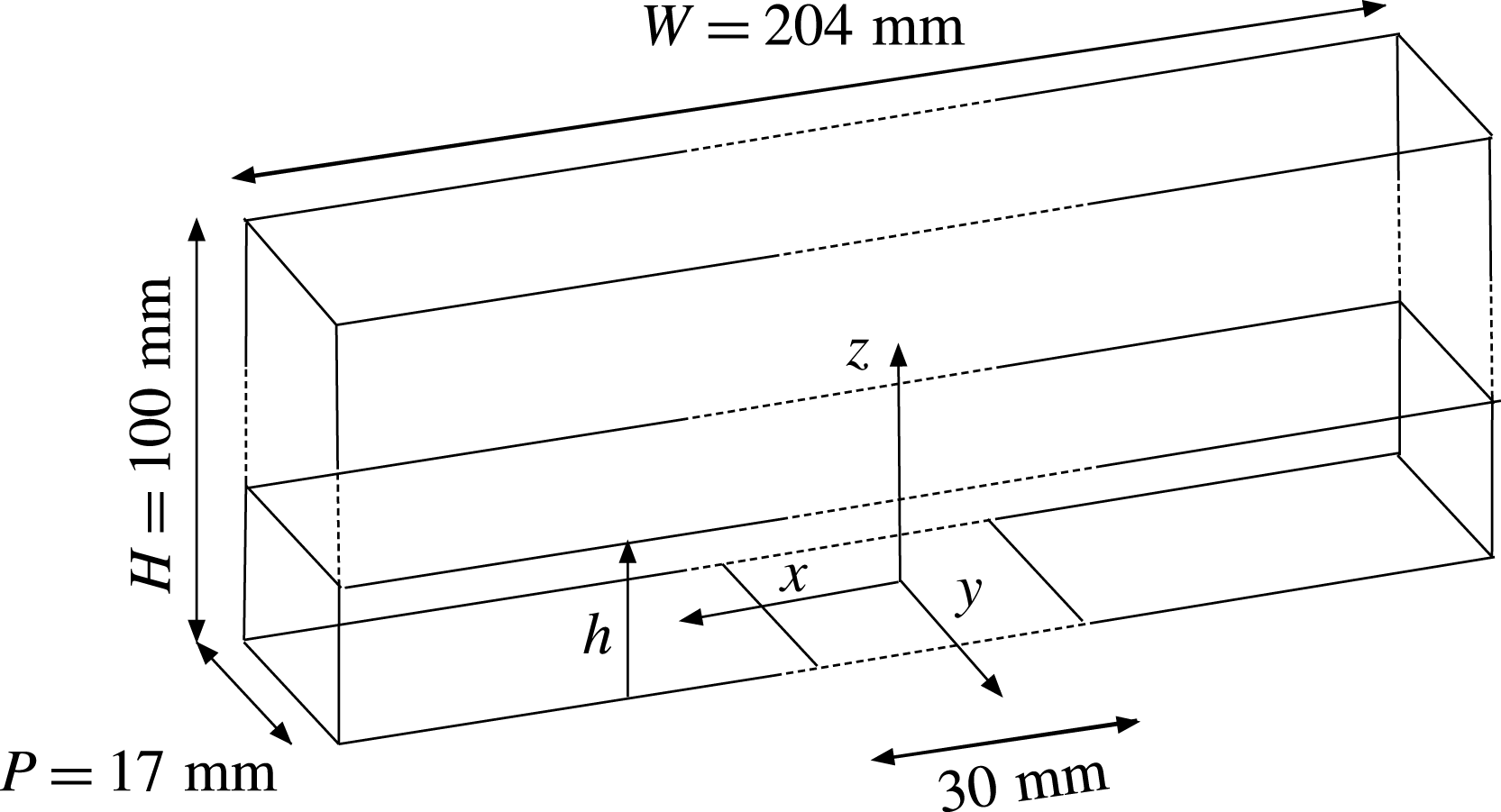
The experimental apparatus consists of a rectangular PMMA box – the tank – with internal dimensions of
 $P=17$
mm in width,
 $W=204$
mm in length and
 $H=100$
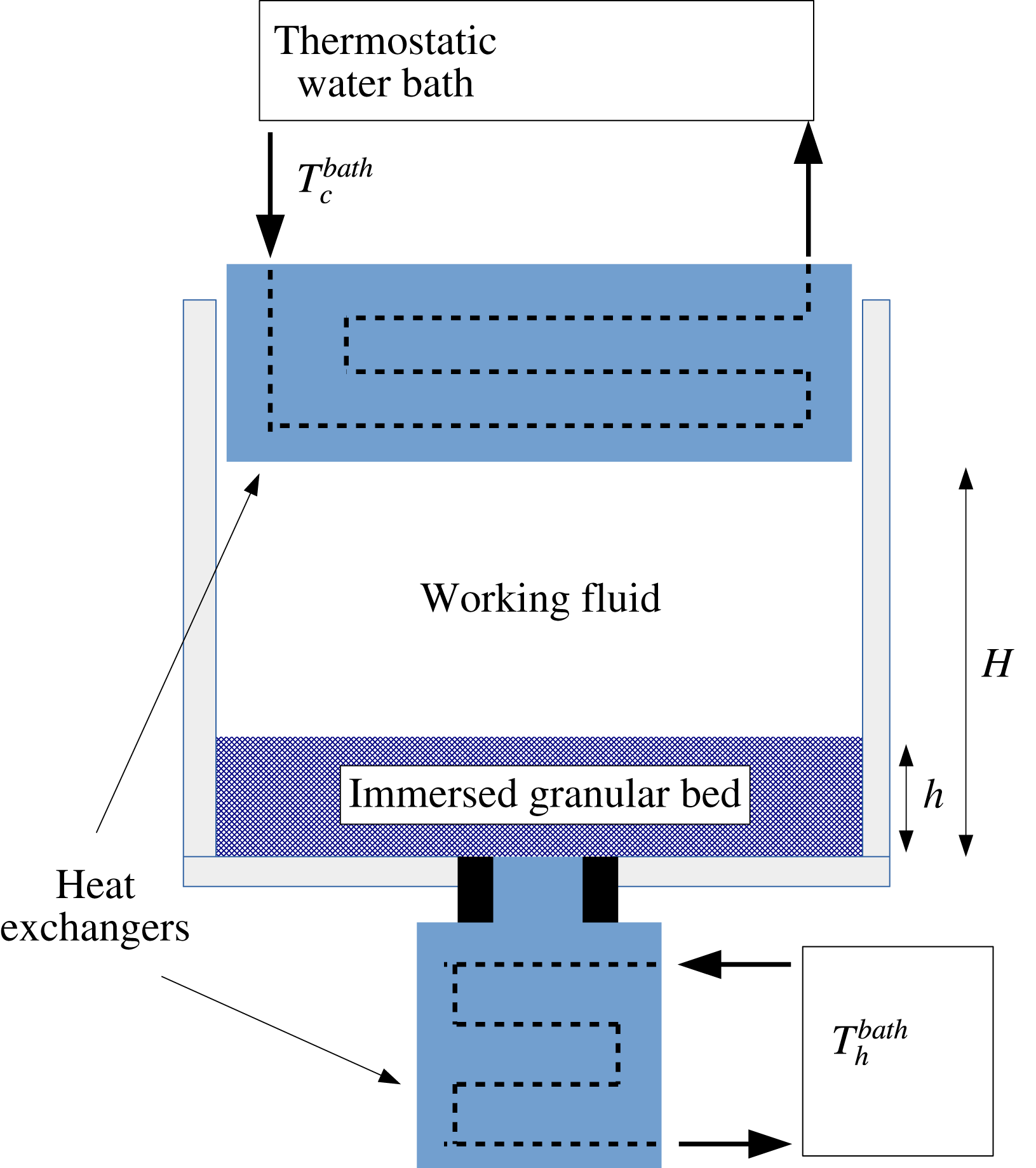
mm in height, that can be locally heated from below. A schematic of the apparatus is shown in figure 1. The
 $z$
coordinate is vertical and the plane
 $z=0$
corresponds to the bottom of the tank. The origin of coordinates corresponds to the centre of the heat exchanger. The
 $x$
and
 $y$
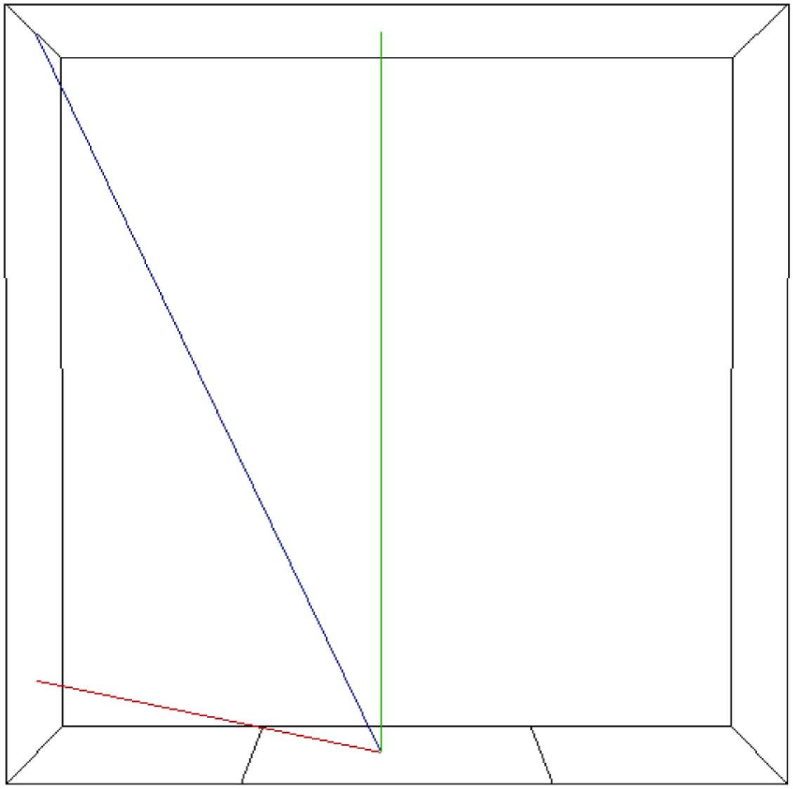
coordinates are respectively the longitudinal and transversal coordinates, as shown in figure 2, depicting the box inner domain sketch. While the other sides of the box are at room temperature
 $T_{room}\simeq 20\,^{\circ }\text{C}$
, the upper side
 $z=H$
is made of a copper plate and maintained at a fixed, lower temperature
 $T_{c}=15\,^{\circ }\text{C}$
. The room temperature is always larger than the upper temperature:
 $T_{room}>T_{c}$
. The inner mixture can be heated from below by a 30 mm wide copper plate located in the middle of the bottom of the tank and of the same (17 mm) width (see the global sketch in figure 2). Each plate is respectively connected to two temperature controlled water baths. Continuous water circulation allows for fixed-temperature boundary conditions. Both plates temperatures are monitored using platinum probes inserted into the plates. In the following, we shall respectively refer to the upper (cold) and lower (hot) plates temperatures as
 $T_{c}$
and
 $T_{h}$
with
 $\unicode[STIX]{x0394}T(t,z)=T(z)-T_{c}$
,
 $\unicode[STIX]{x0394}T(t,z=0)=T_{h}-T_{c}$
. The time
 $t$
denotes the time after heat actually reaches the bed’s bottom surface. The origin of
 $t$
is hence set at the time (denoted
 $\unicode[STIX]{x1D70F}_{ii}$
in § 3.4) when heat actually reaches the granular bed’s bottom. Typically,
 $T_{h}\simeq 40$
–
 $60\,^{\circ }\text{C}$
. The incoming heat flux,
 $\dot{q}_{in}$
, from the bottom is measured separately, using a fluxmeter probe that fits the bottom heat exchanger, with a sensitivity of
 $2.7~\unicode[STIX]{x03BC}\text{V}~\text{W}^{-1}~\text{m}^{-2}$
. We use spherical monodisperse polystyrene particles of diameter
 $D=250~\unicode[STIX]{x03BC}\text{m}$
at room temperature, and with a temperature-dependent density
 $\unicode[STIX]{x1D70C}_{g}$
. The working fluid is water mixed with 6.5 % wt of CaCl
 $_{2}$
salt, in order to increase the fluid density and ease thermal destabilization. The density difference between the above salt water and the saturated granular mixture is
 $\unicode[STIX]{x0394}\unicode[STIX]{x1D70C}^{c}=7.1\pm 0.2~\text{kg}~\text{m}^{-3}$
at the reference (cold) temperature
 $15\,^{\circ }\text{C}$
. Following Zhang, Chen & Han (Reference Zhang, Chen and Han1997) the viscosity of a 6.5 % wt aqueous mixture of CaCl
 $_{2}$
is 25 % higher than that of pure water. Initially, after dispersing the grains into the salted bath, the polystyrene particles are allowed to gently settle at the bottom of the box, to form a loose randomly packed granular bed at the bottom of the tank, with an almost planar surface of height
 $h$
(see figures 1 and 2). The initial average height
 $h$
ranges from 1 to 30 mm. The loose packing fraction of cohesionless frictional spheres is known to decrease with
 $\unicode[STIX]{x1D707}_{S}$
, the mean static friction coefficient (Farrell, Martini & Menon Reference Farrell, Martini and Menon2010). Following the method based on a rolling drum proposed by Courrech du Pontet al. (Reference Courrech du Pont, Gondret, Perrin and Rabaud2003), we found
 $\unicode[STIX]{x1D707}_{S}=\tan \unicode[STIX]{x1D703}_{max}=0.6\pm 0.1$
, with
 $\unicode[STIX]{x1D703}_{max}$
the maximum angle that can be sustained by the granular media at rest, leading to the estimate
 $\unicode[STIX]{x1D719}_{p}\approx 0.56\pm 0.10$
for the initial packing density. In the initial configuration, after particles have settled, and since
 $T_{room}>T_{c}$
, the upper fluid is not completely quiescent. A slow (
 ${\sim}$
a few
 $\text{mm}~\text{s}^{-1}$
) large scale recirculation (LSR) can be observed: the inner fluid is cooled down using both exchangers at
 $T_{c}=15\,^{\circ }\text{C}$
but the lateral walls are heated by the room.
Schematic of the experimental set-up. The heating coil appears at the bottom while a water circulation allows for refrigeration in the upper side.

Schematic of the inner domain with axis and dimensions. The length of the hot plate is 30 mm.

Before heating starts, downflow is observed within the central region of the tank, while upflow occurs at both side walls. The experiment (i.e. the localized heating of the lower plate) is initiated at least one hour after
 $\unicode[STIX]{x0394}T$
is observed to reach its steady (initial) state (
 $\unicode[STIX]{x0394}T=0$
). As can be observed in supplementary movie 1 available at https://doi.org/10.1017/jfm.2018.141 (a movie of the destabilization process), the initial slow LSR remains unchanged until the granular layer is destabilized and this shows that the thermal boundary layer (TBL) inside the granular bed does not thermally influence the water/bed interface before destabilization occurs. Since the fluid is locally heated from below at the centre of the plate, the direction of rotation of the fluid would have been reversed if the TBL reached the interface before the destabilization and started heating the fluid just above the interface.
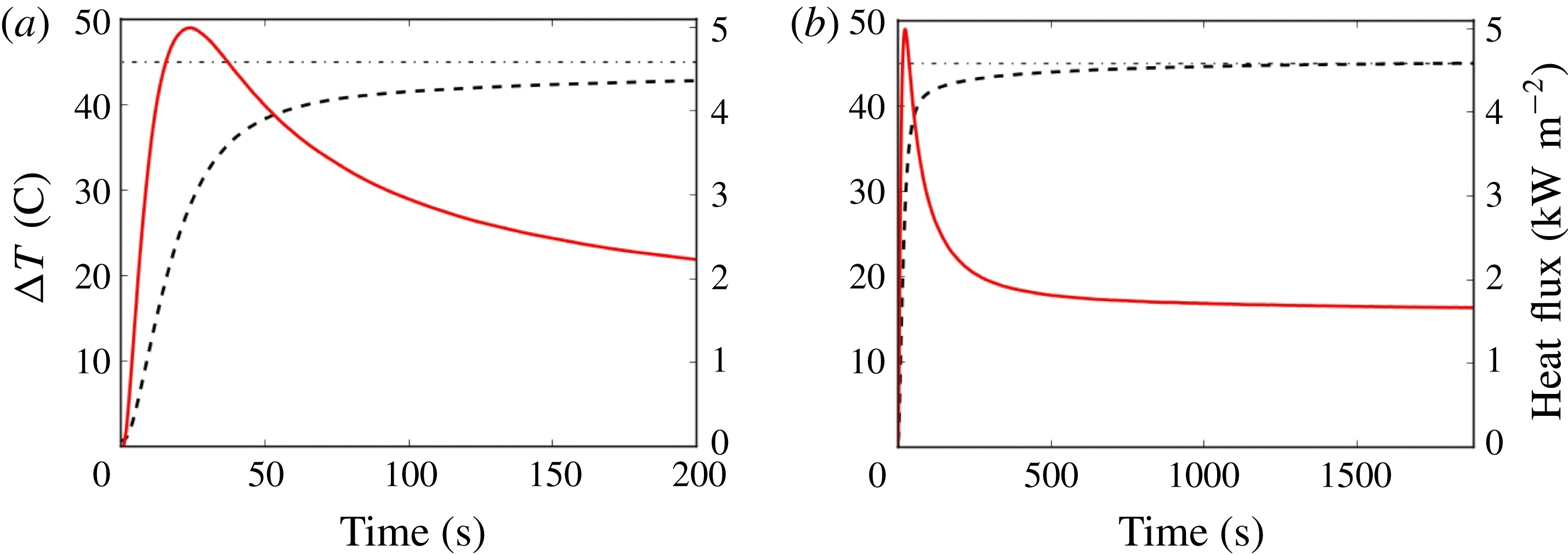
In order to access the initial transient regime and discuss the vertical profile of the temperature for early times, we have equipped the experimental set-up with a heat flux sensor at the lower heat exchanger. Initiation of a typical experiment is triggered by connecting the hot water bath to the bottom heat exchanger. This very sharply increases
 $\unicode[STIX]{x0394}T(t,z=0)$
while the top heat exchanger is maintained at the constant reference temperature
 $T_{c}$
(see figure 3). In order to consistently define the intensity
 $\unicode[STIX]{x1D6E5}$
of the forcing, we use the value of
 $\unicode[STIX]{x0394}T$
in the long run (
 $\text{Time}\sim 10^{3}~\text{s}$
):
 $\unicode[STIX]{x1D6E5}=\unicode[STIX]{x0394}T(t\rightarrow \infty ,z=0)$
, which corresponds to a heat flux
 $\dot{q}_{in}$
of approximately
 $1.8~\text{kW}~\text{m}^{2}$
. The intensity
 $\unicode[STIX]{x1D6E5}$
can be measured by using a sufficiently high
 $\unicode[STIX]{x0394}\unicode[STIX]{x1D70C}^{c}$
ensuring the stability of the granular layer while
 $\unicode[STIX]{x0394}T$
attains its asymptotic value and can be modified by varying the temperature of the hot water bath. As studied in Morize et al. (Reference Morize, Herbert and Sauret2017), the maximum slope of
 $\unicode[STIX]{x0394}T$
(see figure 3) is affected by the value of
 $\unicode[STIX]{x1D6E5}$
. In the present study, all experiments are conducted with a fixed value of
 $\unicode[STIX]{x1D6E5}=45~\text{K}$
, therefore we measure a slope of
 $\unicode[STIX]{x1D6FC}\simeq 1.25~\text{K}~\text{s}^{-1}$
.
Time evolution of measured heat flux density (solid lines) and
 $\unicode[STIX]{x0394}T=\unicode[STIX]{x0394}T(t,z=0)$
(dashed lines) for
 $h=10$
mm; the value of
 $\unicode[STIX]{x1D6E5}$
(see text) is represented by the dot-dashed horizontal lines. (a) Early evolution; (b) global time evolution. For the sake of consistency between the different initial layer heights
 $h$
, the time origin (marked as
 $\text{Time}=0$
in the figure) is here chosen as the time (denoted
 $\unicode[STIX]{x1D70F}_{ii}$
, see § 3.4) when heat actually reaches the heating metallic plate, i.e. when both
 $\unicode[STIX]{x0394}T$
and the heat flux sharply depart from zero.
 $\unicode[STIX]{x1D6E5}$
being fixed, the maximal slope value for
 $\unicode[STIX]{x0394}T$
(a) adopts the same initial value
 $\unicode[STIX]{x1D6FC}\simeq 1.25~\text{K}~\text{s}^{-1}$
. Temperature and heat flux both settle after a delay of approximately 700 to 900 s.

3 Granular layer evolution
3.1 Observation of the different stages of the layer evolution
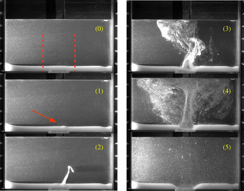
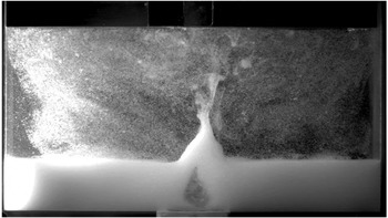
The different stages of the granular layer evolution are shown in figure 4 and can be described as follows. At first (see figure 4(0)), before the experiment is initiated, the temperature profile is almost uniform and constant in the whole experimental inner region. The layer is almost horizontal. The density profile is also almost uniform and constant in each layer but exhibits a sharp discontinuity at the interface of the saturated granular layer with the upper liquid. Once
 $\unicode[STIX]{x0394}T$
starts to increase, the thermal boundary layer grows and the local density, close to the lower plate, decreases. If
 $\unicode[STIX]{x0394}T$
is increased enough and, as a consequence, the granular medium average density decreases enough – by thermal expansion – an initial deformation can be observed at the surface of the granular medium (figure 4(1), see the red arrow). This deformation, visible some time after heating starts (see also movie in supplemental material), consists of circular patterns a few millimetres wide and approximately one millimetre high, and roughly located (but not exactly! see § 3.3) where the granular plume will later emerge. Also notice that the deformation comes with a small layer volume decrease, barely visible on the pictures. While time evolves, the bump amplitude smoothly increases until the complete interface destabilization occurs, with a plume quite steeply arising from the layer (figure 4(2)). After this granular plume suddenly appears, the fluidized layer and plume interact (figure 4(3)) while the erosion step begins (figure 4(4)), stopping once the bottom of the tank is completely uncoated (figure 4(5)). When
 $h$
is large enough, a cavity formation process corresponding to fluidization, can also be observed (see figure 5). In the present paper, we shall only focus on the destabilization process, i.e. until the plume emerges. The erosion, cavity formation and grain re-suspension shall be analysed elsewhere.
Typical destabilization process of the granular layer, here shown for
 $h=10$
mm and
 $\unicode[STIX]{x1D6E5}=45$
K. Destabilization started at
 $t=147$
s. (0)
 $t=0$
: initial situation i.e. up to when heating has just reached the bed’s bottom (the two dotted red vertical lines correspond to the analysed zone for interface evolution monitoring, see text) (1)
 $t=135$
s: precursory deformation of the interface, see the red arrow (2)
 $t=162$
s: granular plume, (3)
 $t=275$
s: plume and beginning of erosion, (4)
 $t=325$
s: erosion and re-deposition of particles and (5) steady (final) stage with particles’ re-deposition left and right from the heating zone and erosion.

Cavity formation at the granular layer, here shown for
 $h=26$
mm and
 $\unicode[STIX]{x1D6E5}=45$
K, 450 s after the destabilization occurs.

In the next paragraph, we shall quantify the time evolution of the granular bed interface.
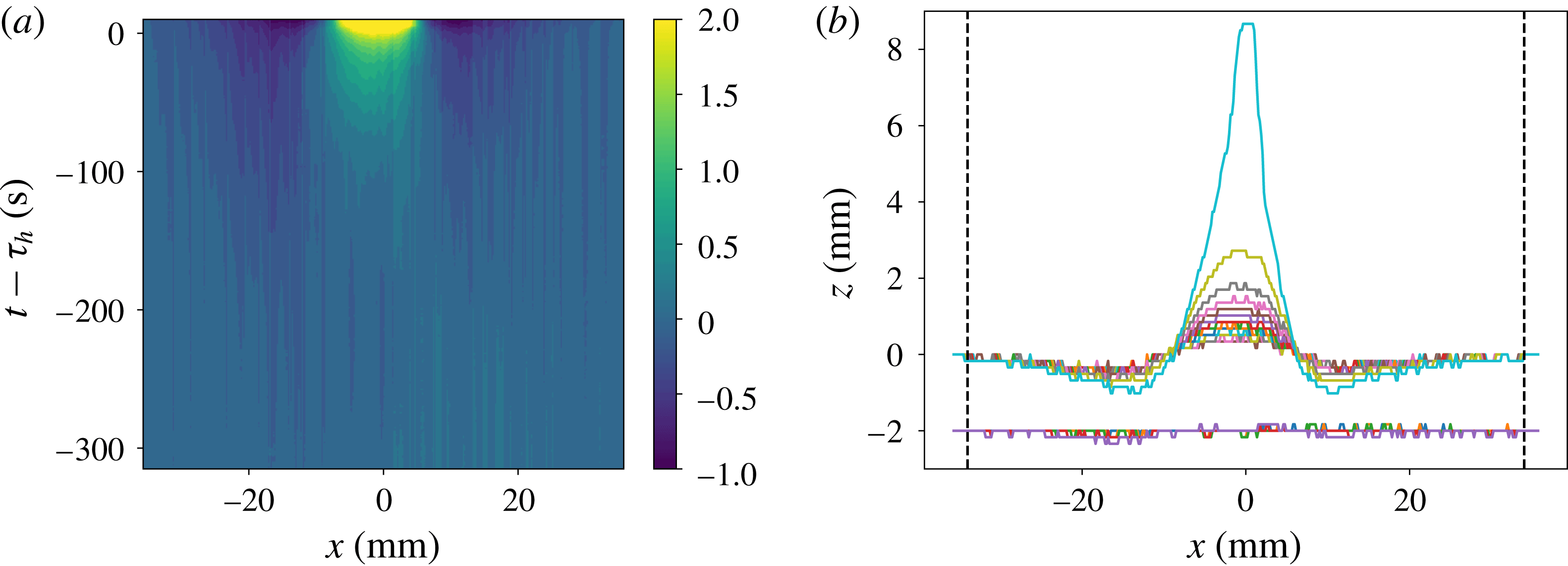
Time evolution of the granular layer upper boundary for
 $h=16$
mm. (a) Spatio-temporal map of the elevation, before the destabilization (at time
 $t-\unicode[STIX]{x1D70F}_{h}=0$
, see text, equation (3.2), for the definition of the destabilization time
 $\unicode[STIX]{x1D70F}_{h}$
). (b) Time evolution of the
 $z$
–
 $x$
elevation profile. As time evolves, the boundary profile tends to grow at the centre (just above the heating plate middle) while deepening in the wings (above the plate edges). Early evolution is drawn each 50 s for
 $t-\unicode[STIX]{x1D70F}_{h}=-315$
to
 $-115$
s (vertically shifted by 2 units for clarity). Later evolution is drawn each 5 s for
 $t-\unicode[STIX]{x1D70F}_{h}=-62.5$
to
 $+7.5$
s. The two vertical dashed axes are located on
 $x=\pm x_{0}$
, where the surface profile is no more disturbed, since the bottom heating plate ranges from
 $-15$
to
 $+15$
mm of the
 $x$
-axis. They are also indicated as the two dotted red vertical lines in figure 4.

3.2 Interface evolution monitoring
In order to record the interface evolution history, one side of the tank is illuminated using a flat vertical laser sheet passing through the middle of the smaller side of the tank. A camera with a typical sampling frequency of a few Hertz then records pictures (
 $1280\times 800$
,
 $170~\unicode[STIX]{x03BC}\text{m}~\text{pixels}^{-1}$
) in a plane normal to the light sheet. In the following we will focus on the two-dimensional (2-D) evolution of the interface before the destabilization occurs. The obtained images are binarized, the threshold being chosen in order to focus on the luminosity contrast at the interface. The typical height variation across the interface is
 $5D$
(with
 $D=250~\unicode[STIX]{x03BC}\text{m}$
the diameter of the particles). The local height
 $z$
of the interface is computed as a function of the
 $x$
-coordinate in the transverse direction, over a large range
 $[-x_{0},x_{0}]$
where deformation occurs (
 $x_{0}=34$
mm, see figure 6).
In order to obtain a single
 $z$
value for each
 $x$
value, and also thanks to the tank’s small width
 $P$
, the interface data used for initial deformation profiles have been filtered with a rolling ball method and the interface is expected to evolve mainly as a 2-D curve. One can compute the now single valued
 $z(x,t)$
. In the following, we shall refer to
 $S(t)$
as the
 $x$
-averaged value
 $S(t)=\int _{-x_{0}}^{+x_{0}}z(x,t)\,\text{d}x$
. The volume (in two dimensions) of the layer will hence be referred as
 $S(t)$
and we shall denote
 $\unicode[STIX]{x0394}S(t)=S(t)-S_{0}$
as the volumetric variation of the layer.
3.3 Layer deformation
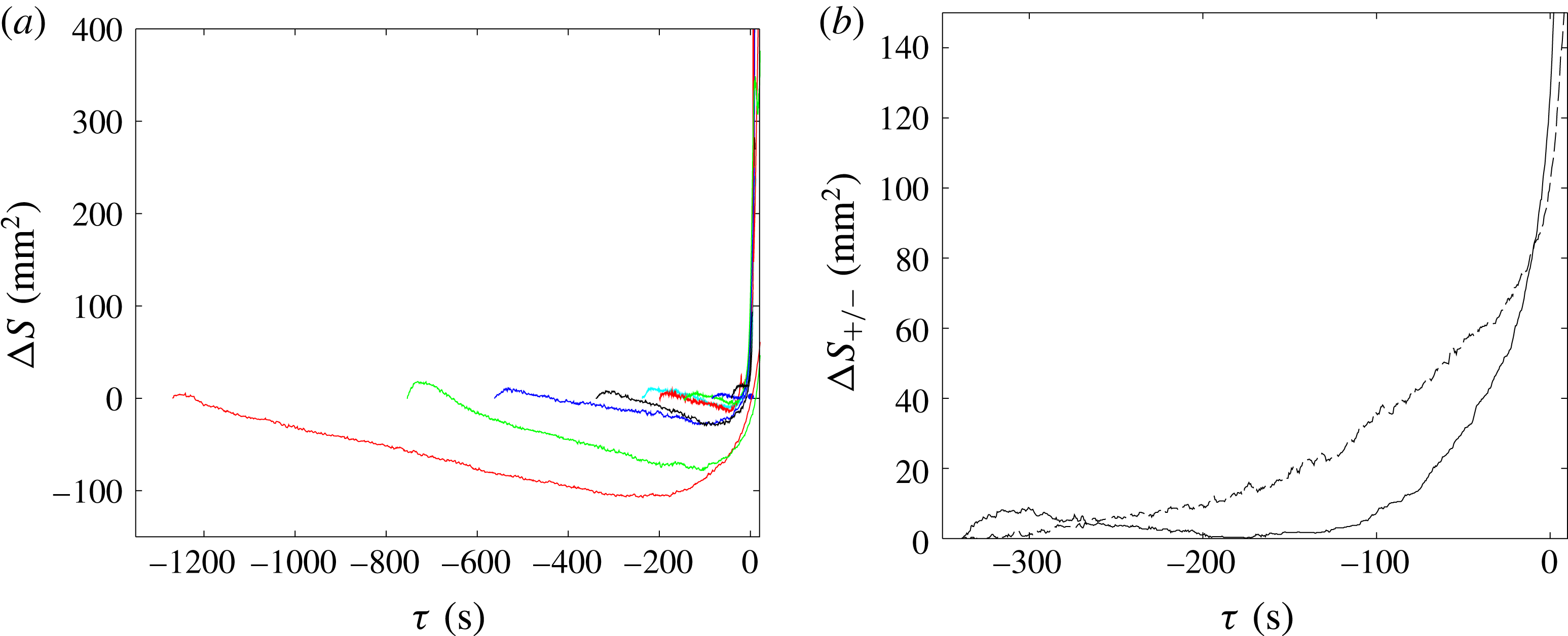
During the early stage, the granular medium seems to act mainly as a passive, purely conductive layer, indicating that no internal dynamics really matters in order to predict the destabilization time. However, the question we would like to address next is the following: does the time history of the layer deformation provide us some information about the internal dynamics of the layer? To start answering this question, we monitored the shape of the layer’s upper boundary, as shown in figure 6. Small but significant modulations of the interface can be clearly observed as soon as the thermal forcing is started. As time evolves, the central height is increasing while both sides tend to deepen. As shown in figure 7(a), at the very beginning of each experiment a small growth in the lower layer’s total volumic variation
 $\unicode[STIX]{x0394}S$
is observed, clearly owing to the early thermal expansion of the granular mixture. Its duration (typically around 30 s) and maximum amplitude (typically a few
 $\text{mm}^{2}$
) are found to be roughly constant for sufficiently large
 $h$
. After this first step, the global volume then decreases almost linearly with time, with a typical slope of
 $0.1~\text{mm}^{2}~\text{s}^{-1}$
.
Interestingly, the volumetric variation of the layer shows that the interface evolution – or the volumic variation – does not correspond only to thermal expansion, but also to local reorganization of the grains and decreases in the layer’s apparent volume, as generally observed with mechanically induced repacking (An et al.
Reference An, Li, Yang, Zou and Yu2009). The positive and negative volumic evolutions of the interface, corresponding to the average effects of local swelling and compaction respectively, are both taken as positive, and denoted
 $\unicode[STIX]{x0394}S_{+}$
and
 $\unicode[STIX]{x0394}S_{-}$
;
 $\unicode[STIX]{x0394}S_{+}$
reads
 $$\begin{eqnarray}\displaystyle \unicode[STIX]{x0394}S_{+}(t)=\int _{-x_{0}}^{x_{0}}\unicode[STIX]{x1D6E4}(x)[z(x,t)-z_{0}(x)]\,\text{d}x, & & \displaystyle\end{eqnarray}$$
with
 $\unicode[STIX]{x1D6E4}(x)=1$
where
 $z(x,t)-z_{0}(x)>0$
and 0 elsewhere and a similar definition holds for
 $\unicode[STIX]{x0394}S_{-}$
. They are both drawn in figure 7(b), for the average initial granular height
 $h=16$
mm. Note that the precision of the measurement of
 $\unicode[STIX]{x0394}S$
is linked to spatial sampling (i.e.
 ${\sim}$
one spherical particle diameter) and the horizontal integration width (
 $2x_{0}=68$
mm). The maximal possible error would therefore be approximately
 $2Dx_{0}=17~\text{mm}^{2}$
. However, since the number of spherical particles along the
 $x$
-direction is approximately
 $400=20^{2}$
, a 5 %-confidence interval (for an assumed Gaussian distribution of errors) yields a more realistic precision of approximately
 $1~\text{mm}^{2}$
, indicating that the represented time evolutions in figure 7 are quite accurate.
The initial deformation is essentially present just above the exchanger, but only appears on average, and is therefore barely visible (at early times) as a specific identifiable structure in figure 6(b). On the other hand, the subsequent sedimentation is more homogeneously distributed on the interface, with a much more specific and visible spatial localization in the figure: one can thus observe a decrease in the vicinity of the ends of the exchanger, and a subsequent growth in its centre. It hence turns out that it is not really possible to accurately define a preferential region leading to the initiation of the plume from the initial swelling, i.e. the initial swelling does not exactly correspond (spatially) to the initiation of the plume. To describe the whole deformation, we will be rather interested in a region of size large (for example double) compared to the length of the exchanger, without favouring one region rather than another. For computing the velocity of the sedimentation front, we shall take the average over this length (
 $2x_{0}$
) of the rate of deformation of the interface.
By separating the positive and negative contributions to
 $\unicode[STIX]{x0394}S$
, we observe that the slow decrease of
 $\unicode[STIX]{x0394}S$
is due to the continuous fall of the granular layer, whilst the growth slows down and stops after the initial deformation. The decrease is finally bounded by
 $\unicode[STIX]{x0394}S_{+}\approx \unicode[STIX]{x0394}S_{-}$
, which is a clear precursor of the plume formation. It is worth noticing that
 $\unicode[STIX]{x0394}S_{-}$
suddenly increases just before the plume emerges, but since the slope of the positive increasing fraction is larger than the slope of the negative one (i.e.
 $\text{d}\unicode[STIX]{x0394}S_{+}/\text{d}t>\text{d}\unicode[STIX]{x0394}S_{-}/\text{d}t$
), the volume fraction
 $\unicode[STIX]{x1D719}$
is dramatically reduced.
(a) Time evolution of the granular layer total apparent volumetric variation
 $\unicode[STIX]{x0394}S$
, for
 $h=30~\text{mm}$
, 23 mm, 20 mm, 16 mm, 12 mm, 10 mm and 8 mm respectively (from left to right). (b) Time evolution of the positive and negative parts,
 $\unicode[STIX]{x0394}S_{+}$
(solid) and
 $\unicode[STIX]{x0394}S_{-}$
(dashed), both taken as positive, of the volumetric evolution of the layer interface, for
 $h=16$
mm. For the sake of clarity, we choose a common
 $\unicode[STIX]{x1D70F}=t-\unicode[STIX]{x1D70F}_{h}=0$
time for all curves (plotted on the left) by defining the origin of time
 $\unicode[STIX]{x1D70F}$
as the instant when
 $\unicode[STIX]{x0394}S_{+}=\unicode[STIX]{x0394}S_{-}$
for
 $h=30$
mm.

3.4 Times
 $\unicode[STIX]{x1D70F}_{h}$
and
$\unicode[STIX]{x1D70F}_{h}^{\star }$


In figure 7, one can notice that the granular layer total apparent volume starts to increase again just before the triggering of the granular plume and the apparent volume reaches its absolute minimum. This behaviour stems from the obtained contour of the dynamics of the bed’s interface, and this qualitative profile does not depend of the specific choice of the used value of
 $x_{0}$
for the apparent surface computation (see figure 7), provided
 $x_{0}$
is large enough (say at least twice) compared to the heating plate half-length. The present exploitation hence allows us to identify several remarkable times in the experiment, that may, or may not, be easily accessible experimentally:
(i) the time
$\unicode[STIX]{x1D70F}_{i}$
when heating is triggered, which is directly accessible in our experiment. However,
$\unicode[STIX]{x1D70F}_{i}$
is not physically relevant, since we do not know when heat actually reaches the granular bed’s bottom. Moreover, in real systems,
$\unicode[STIX]{x1D70F}_{i}$
is generally not accessible, nor really significant,(ii) the time
$\unicode[STIX]{x1D70F}_{ii}$
when heat actually reaches the granular bed’s bottom;
$\unicode[STIX]{x1D70F}_{ii}$
is physically relevant but may be hardly accessible in real-life systems, like in geophysics. This instant
$\unicode[STIX]{x1D70F}_{ii}$
had been chosen as the origin of times in figure 3,(iii) the time
$\unicode[STIX]{x1D70F}_{iii}$
when the apparent volume of the bed is observed to reach its early local maximum (see figure 7
a). The physical relevance of
$\unicode[STIX]{x1D70F}_{iii}$
is questionable, and when
$h$
is not large enough (here for
$h\leqslant$
8 mm), the local maximum of the volume variation may be barely visible, if even existent. However, for large enough depths
$h$
, its experimental highlighting is relatively easier. In our experiments, we observed that, for large enough
$h$
, the duration
$\unicode[STIX]{x1D70F}_{iii}-\unicode[STIX]{x1D70F}_{ii}$
was small (compared to the total destabilization time);
$\unicode[STIX]{x1D70F}_{ii}$
is the physically relevant time and
$\unicode[STIX]{x1D70F}_{iii}$
seems a fair estimation of
$\unicode[STIX]{x1D70F}_{ii}$
,(iv) the time
$\unicode[STIX]{x1D70F}_{iv}$
when the apparent volume of the bed is observed to reach its global minimum (as is apparent in figure 7
a) The physical relevance of
$\unicode[STIX]{x1D70F}_{iv}$
is clear: at time
$\unicode[STIX]{x1D70F}_{iv}$
, the local reorganization/sedimentation of the grains is superseded by the bed’s thermal dilation, indicating the start of the actual buoyant destabilization process,(v) the time
$\unicode[STIX]{x1D70F}_{v}$
when the apparent volume variation of the bed vanishes again (see again figure 7
a) i.e. the apparent volume increases and reaches its initial value;
$\unicode[STIX]{x1D70F}_{v}$
is very close to the time
$\unicode[STIX]{x1D70F}_{vi}$
when the destabilization plume suddenly emerges. While
$\unicode[STIX]{x1D70F}_{vi}$
is hard to define precisely and unambiguously, it is easy to identify and measure, since destabilization occurs very sharply, and
$\unicode[STIX]{x1D70F}_{v}\lesssim \unicode[STIX]{x1D70F}_{vi}$
is a well-defined, accurate approximation of
$\unicode[STIX]{x1D70F}_{vi}$
.


The destabilization time initially proposed in Morize et al. (Reference Morize, Herbert and Sauret2017) was
 $\unicode[STIX]{x1D70F}=\unicode[STIX]{x1D70F}_{vi}-\unicode[STIX]{x1D70F}_{ii}$
, a first natural way to define it. In the present work, we shall still define the destabilization time
 $\unicode[STIX]{x1D70F}_{h}$
as
 $$\begin{eqnarray}\displaystyle \unicode[STIX]{x1D70F}_{h}=\unicode[STIX]{x1D70F}_{vi}-\unicode[STIX]{x1D70F}_{ii}\simeq \unicode[STIX]{x1D70F}_{v}-\unicode[STIX]{x1D70F}_{ii} & & \displaystyle\end{eqnarray}$$
since
 $\unicode[STIX]{x1D70F}_{v}$
is very close to the time
 $\unicode[STIX]{x1D70F}_{vi}$
introduced above. In the present work, the actually analysed time
 $\unicode[STIX]{x1D70F}_{h}$
is
 $\unicode[STIX]{x1D70F}_{h}=\unicode[STIX]{x1D70F}_{v}-\unicode[STIX]{x1D70F}_{ii}$
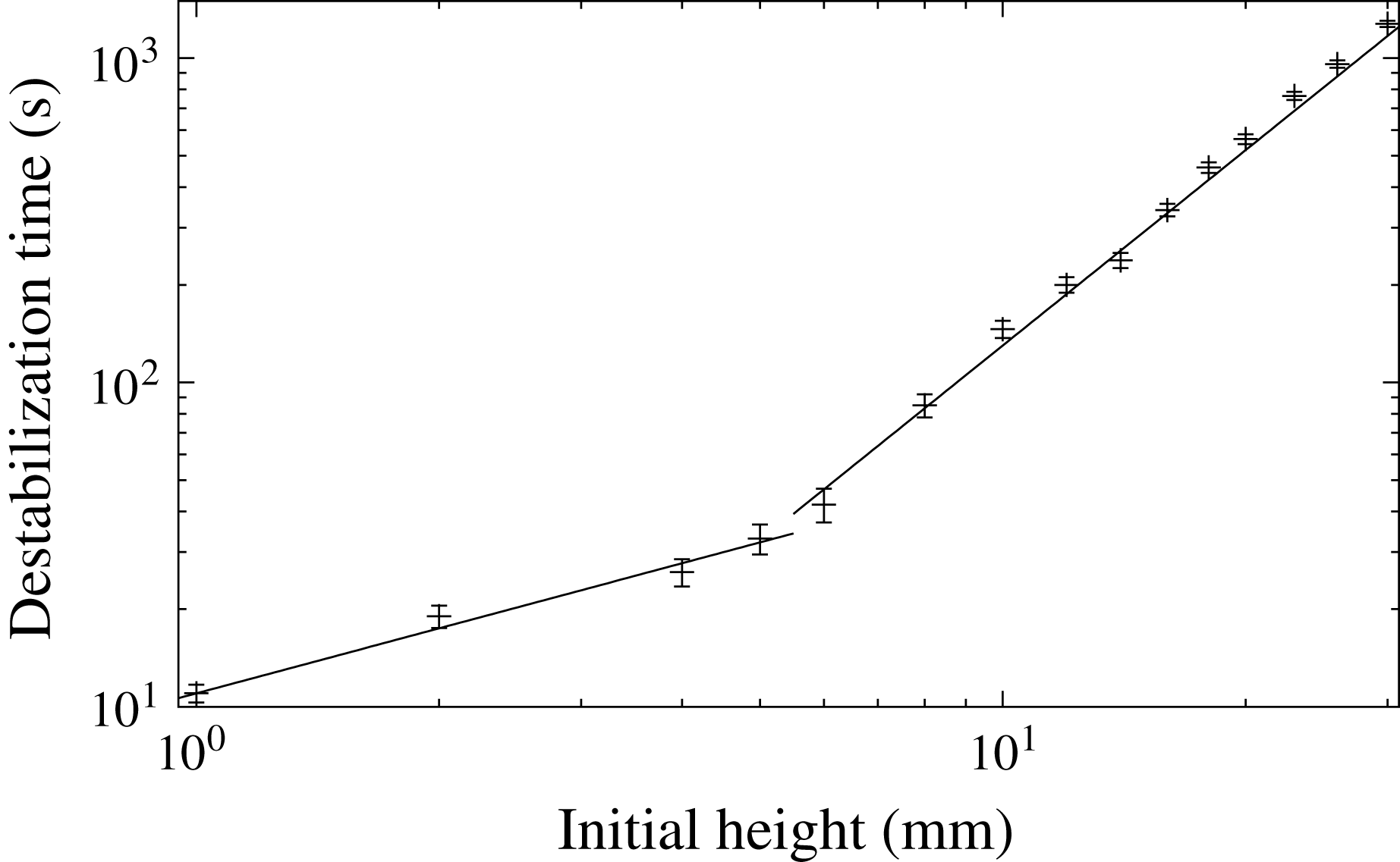
. We first report in figure 8 the variation of
 $\unicode[STIX]{x1D70F}_{h}$
with respect to the granular bed initial height
 $h$
.
In real systems, however, like in geophysics, while the monitoring of the surface evolution is in general experimentally accessible, the modification of the thermal conditions at the edges, that is to say in depth, is much less so. We hence build on the volume variation evolutions (drawn in figure 7
a) to propose another characteristic time, denoted
 $\unicode[STIX]{x1D70F}_{h}^{\star }$
, and bounded by the extrema (maximum and minimum) of
 $\unicode[STIX]{x0394}S$
. Thanks to the above definitions of the characteristic times,
 $\unicode[STIX]{x1D70F}_{h}^{\star }$
is defined as:
 $$\begin{eqnarray}\displaystyle \unicode[STIX]{x1D70F}_{h}^{\star }=\unicode[STIX]{x1D70F}_{iv}-\unicode[STIX]{x1D70F}_{iii}. & & \displaystyle\end{eqnarray}$$
Note that
 $\unicode[STIX]{x1D70F}_{h}^{\star }$
is solely based on quantities endogenous to the evolution of the bed: the shape of the bed interface and the spatial integration of its internal reorganizations. Also note that when the apparent volume variation starts to increase again, the effect of the spatial reorganization/sedimentation of the grain becomes negligible compared to the thermal swelling of the bed, a clear signature that the thermal destabilization process actually begins. This naturally leads to consider
 $\unicode[STIX]{x1D70F}_{h}^{\star }$
only for the experiments for which the destabilization time (since
 $\unicode[STIX]{x1D70F}_{h}\gtrsim \unicode[STIX]{x1D70F}_{h}^{\star }$
) is large enough to allow the volume to reach these extrema: in the present situation, for
 $h\geqslant 8$
mm.
For the destabilization time
 $\unicode[STIX]{x1D70F}_{h}$
, one can observe two different regimes. A first regime, for large enough
 $h$
, follows a power law with an exponent of 2,
 $\unicode[STIX]{x1D70F}_{h}\propto h^{2}$
, as already reported in Morize et al. (Reference Morize, Herbert and Sauret2017). For smaller
 $h$
values (
 $h\lesssim 5$
mm), a second identified regime yields a different power law exponent:
 $\unicode[STIX]{x1D70F}_{h}\propto h^{\unicode[STIX]{x1D714}}$
, with
 $\unicode[STIX]{x1D714}\sim 2/3$
. In § 4.2, we shall propose scenarios able to quantitatively capture the
 $\unicode[STIX]{x1D70F}_{h}(h)$
behaviour.
In figure 9(a), we report, for large enough
 $h$
, the characteristic time
 $\unicode[STIX]{x1D70F}_{h}^{\star }$
. We observe that, for
 $h$
values smaller than 23 mm, the behaviour of
 $\unicode[STIX]{x1D70F}_{h}^{\star }(h)$
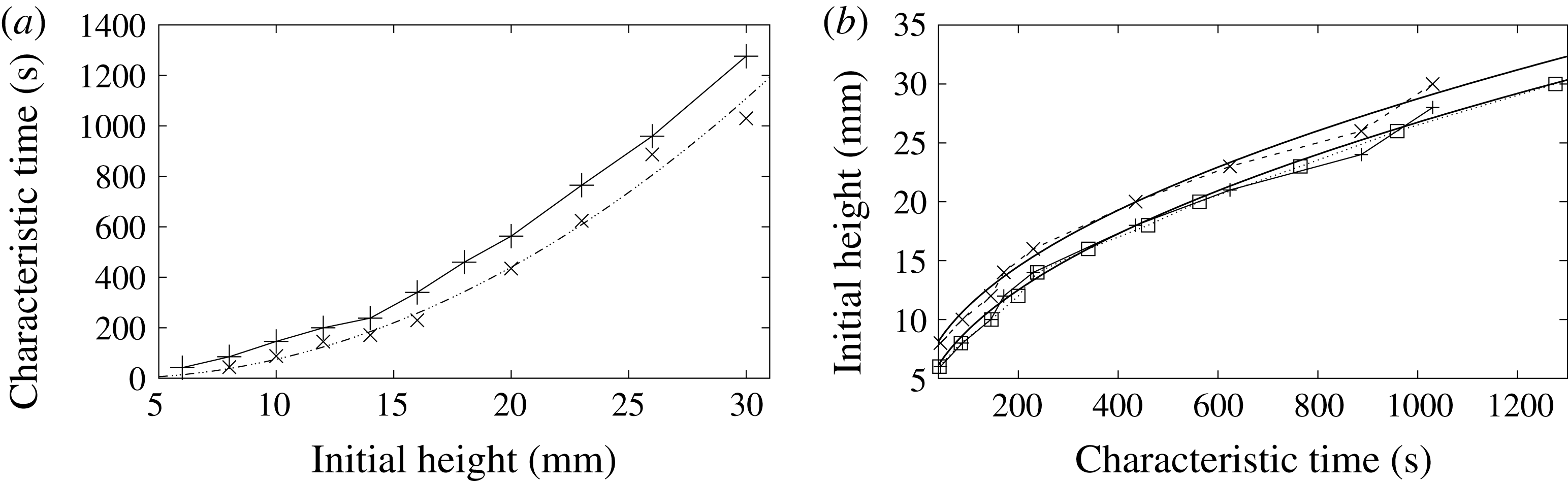
is clearly quadratic, as evidenced in figure 9(a). Moreover, and interestingly enough, we observe that the values of
 $\unicode[STIX]{x1D70F}_{h}^{\star }(h)$
, when
 $h$
is shifted by 2 mm, seem to coincide quite accurately with the
 $\unicode[STIX]{x1D70F}_{h}(h)$
(quadratic) curve, for
 $8\leqslant h\leqslant 23$
mm (the squares in figure 9(b) represent 2 mm shifted values of
 $\unicode[STIX]{x1D70F}_{h}^{\star }$
). This tends to show that
 $\unicode[STIX]{x1D70F}_{h}^{\star }$
captures exactly the same conductive history as
 $\unicode[STIX]{x1D70F}_{h}$
, but represents a characteristic effective heating time for destabilization, excluding the duration of actual mechanical destabilization. This remark may be of some valuable interest in other contexts, where the min and max values of the bed layer may be accessible, e.g. in volcanology, when testing the stability of the mush of a magmatic chamber. The present introduced times – in particular
 $\unicode[STIX]{x1D70F}_{h}^{\star }$
– can be connected to a regime of magmatic eruptions triggered by buoyancy, as identified in Degruyter & Huber (Reference Degruyter and Huber2014) (see § A.3).
Observed destabilization times
 $\unicode[STIX]{x1D70F}_{h}$
as a function of the initial granular layer thickness
 $h$
. Measure errors were estimated as one half of
 $\unicode[STIX]{x1D70F}_{v}-\unicode[STIX]{x1D70F}_{ii}$
(for large enough
 $h$
, see § 1) and to a few seconds for small
 $h$
. The two lines slopes are respectively
 $2/3$
and 2.

(a) Observed characteristic effective heating times for destabilization
 $\unicode[STIX]{x1D70F}_{h}^{\star }$
(
 $\times$
symbols) as compared to destabilization times
 $\unicode[STIX]{x1D70F}_{h}$
(
 $+$
symbols and solid line), both as functions of the initial granular layer thickness
 $h$
. The
 $\cdots \,$
—
 $\cdots \,$
line is a least-square quadratic interpolation (
 $1.51\times (h-2.96)^{2}$
) of the 8 first points of
 $\unicode[STIX]{x1D70F}_{h}^{\star }$
(
 $8\leqslant h\leqslant 23$
mm). (b) Initial heights of the granular bed as a function of characteristic times:
 $\unicode[STIX]{x1D70F}_{h}$
(squares and dotted line),
 $\unicode[STIX]{x1D70F}_{h}^{\star }$
(
 $\times$
and dashed line). The
 $+$
symbols represents the
 $h$
values corresponding to
 $\unicode[STIX]{x1D70F}_{h}^{\star }$
, shifted by 2 mm. The two solid curves are least square quadratic interpolations: respectively
 $h=\unicode[STIX]{x1D708}$
(
 $\unicode[STIX]{x1D70F}+3$
) and
 $h=\unicode[STIX]{x1D708}$
(
 $\unicode[STIX]{x1D70F}+1$
), with
 $\unicode[STIX]{x1D708}\simeq 0.814$
.

4 Discussion, proposed scenarios
4.1 Description
After the hot water circulation is triggered, and after a short delay (
 ${\sim}$
10–20 s, depending on
 $h$
, and corresponding to the duration
 $\unicode[STIX]{x1D70F}_{ii}-\unicode[STIX]{x1D70F}_{i}$
), the temperature of the plate underneath rises very quickly, and heat starts to diffuse through the granular layer, as shown in figure 3. At first, one can think of three interactions counteracting the grains’ motion, namely the solid friction between the solid spheres, the viscous drag due to shearing in the very thin film of water between the areas of contact and cohesive forces. However, when heat diffuses and temperature increases, since the thermal dilatation coefficient of water is higher than of polystyrene, the interstitial water tends to increase the lubrication film thickness as well as the interstitial pressure between the spheres, with the consequence being a decrease in local resistance viscosity of the granular layer. Another consequence is the observed swelling at the layer interface: the stacked spheres will also dilate but at the same time, perturbed by the expansion of the liquid, they will move and tend to settle towards a more compact packing through a local liquefaction behaviour. The observed net effect is that the total volume of the bed decreases, with water being expelled from the lower layer. In this lubricated situation, the granular rigidity due to pure solid friction disappears and the main behaviour is quickly driven by buoyant forces, as we shall show now.
4.2 Conductive modelling
We take the Boussinesq approximation for buoyancy. Assuming a constant averaged thermal expansion coefficient
 $\unicode[STIX]{x1D6FD}_{m}$
for the lower layer medium, the local (averaged) density of the granular mixture (grains+liquid)
 $\unicode[STIX]{x1D70C}_{m}$
is given by
 $$\begin{eqnarray}\displaystyle \unicode[STIX]{x1D70C}_{m}=\unicode[STIX]{x1D70C}_{m}^{c}(1-\unicode[STIX]{x1D6FD}_{m}(T-T_{c})), & & \displaystyle\end{eqnarray}$$
where
 $\unicode[STIX]{x1D70C}_{m}^{c}$
and
 $T_{c}$
are respectively taken as reference (cold) values (see below) for density and temperature for the above local linear approximation (4.1).
In order to be destabilized, the height-averaged density of the heated bubble should diminish and reach the value corresponding to the surrounding cold fluid
 $\unicode[STIX]{x1D70C}_{l}^{c}$
:
 $$\begin{eqnarray}\displaystyle \frac{1}{{\mathcal{V}}}\int _{{\mathcal{V}}}\unicode[STIX]{x1D70C}_{m}\,\text{d}{\mathcal{V}}-\unicode[STIX]{x1D70C}_{l}^{c}=\frac{1}{{\mathcal{V}}}\int _{{\mathcal{V}}}(\unicode[STIX]{x1D70C}_{m}-\unicode[STIX]{x1D70C}_{l}^{c})\,\text{d}{\mathcal{V}}=0, & & \displaystyle\end{eqnarray}$$
where
 ${\mathcal{V}}$
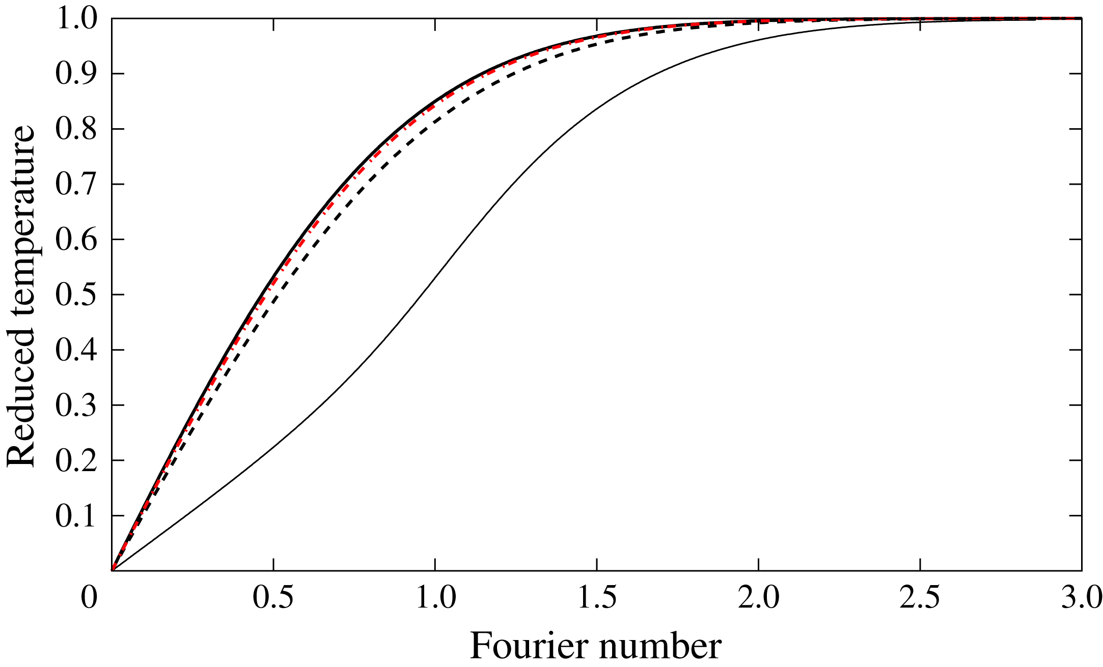
denotes the volume encompassing the heated lower layer and the part of the bed above it. For a purely conductive process, and depending on the boundary conditions (fixed or evolving temperature and heat flux along the metallic bottom plate), the temperature profile depends only on the Fourier number
 $r^{2}/D_{th}t$
, where
 $D_{th}$
is the average thermal diffusivity of the saturated granular layer, and
 $r$
a spatial coordinate. Note that the thermal diffusivities of the polystyrene spheres and the surrounding salted water are almost constant and of the same order (
 ${\sim}1.5\times 10^{-7}~\text{m}^{2}~\text{s}^{-1}$
) across the temperature range considered, allowing an homogeneous local temperature field for the saturated mixture.
For the sake of simplicity, let us first assume a one-dimensional temperature profile in the lower layer,
 $T(z,t)$
. Preliminary measurements and 3-D numerical simulations of purely conductive solids, either with fixed or evolving
 $T_{h}$
temperature boundary conditions, showed that the temperature profile along the central vertical axis actually fits very well to a 1-D expression, with a fixed
 $T_{h}$
value.
Hence, the expression reads:
 $$\begin{eqnarray}\displaystyle \frac{T(z,t)-T_{h}}{T_{c}-T_{h}}=\text{erf}\left(\frac{z}{2\sqrt{D_{th}t}}\right), & & \displaystyle\end{eqnarray}$$
where
 $z$
is the ascending vertical coordinate (with, as stated above, the origin
 $z=0$
at the lower plate level),
 $t=|\unicode[STIX]{x1D70F}_{h}-\unicode[STIX]{x1D70F}|$
the (positive) time after heating starts, and erf denotes the error function. If
 $\unicode[STIX]{x1D6FD}_{m}$
is assumed constant,
 $$\begin{eqnarray}\displaystyle \unicode[STIX]{x1D70C}_{m}-\unicode[STIX]{x1D70C}_{l}^{c}=\unicode[STIX]{x1D70C}_{m}^{c}\left(1-\unicode[STIX]{x1D6FD}_{m}(T_{h}-T_{c})\text{erf}\left(\frac{z}{2\sqrt{D_{th}t}}\right)\right)-\unicode[STIX]{x1D70C}_{l}^{c}. & & \displaystyle\end{eqnarray}$$
Note that
 $\unicode[STIX]{x1D70C}_{m}^{c}$
is the density of the granular mixture at
 $T=T_{ref}=T_{c}$
:
 $\unicode[STIX]{x1D70C}_{m}^{c}=\unicode[STIX]{x1D70C}_{m}(T_{c})>\unicode[STIX]{x1D70C}_{l}^{c}$
. Now, integrating equation (4.4) over
 $z$
from
 $z=0$
to
 $z=h$
(the lower layer height) and dividing by
 $\sqrt{D_{th}t}$
leads to an expression depending on
 $\unicode[STIX]{x1D701}=h/\sqrt{D_{th}t}$
only: criterion (4.2) yields an equation of the form
 ${\mathcal{F}}(\unicode[STIX]{x1D701})=0$
. The positive root
 $\unicode[STIX]{x1D701}_{0}$
of
 ${\mathcal{F}}(\unicode[STIX]{x1D701})$
corresponds to the destabilization time
 $\unicode[STIX]{x1D70F}_{h}=(h/\unicode[STIX]{x1D701}_{0})^{2}/D_{th}$
given by criterion (4.2). This first approach, that we shall refer to as one-dimensional homogenized model, leads to the correct conductive scaling for the estimated destabilization time
 $\unicode[STIX]{x1D70F}_{h}\sim h^{2}/D_{th}$
, as already identified in Morize et al. (Reference Morize, Herbert and Sauret2017).
In a second step, we can go further and try to get quantitative results. Indeed, a slightly more elaborate criterion – but still simple enough for analytic treatment – allows us to reproduce the observed destabilization times strikingly well, when varying the initial granular layer height
 $h$
(for
 $h>5$
mm). The modelling now includes the temperature dependence of the dilatation coefficient of the lower granular saturated layer, and also takes into account the multi-dimensional aspect.
Let assume a locally averaged value for density in the lower layer,
 $\bar{\unicode[STIX]{x1D70C}}=\unicode[STIX]{x1D719}_{p}\unicode[STIX]{x1D70C}_{g}+(1-\unicode[STIX]{x1D719}_{p})\unicode[STIX]{x1D70C}_{l}$
, with
 $\unicode[STIX]{x1D719}_{p}$
the initial packing density. As already mentioned, the calculated value
 $\unicode[STIX]{x1D719}_{p}=0.56\pm 0.10$
corresponds to a very loose random packing of slowly settling spheres. Since the temperature variation range remains small (from 15 to
 $45\,^{\circ }\text{C}$
), the temperature-dependent salt water thermal expansion coefficient
 $\unicode[STIX]{x1D6FD}_{l}$
is approximated through a first-order Taylor expansion in temperature:
 $\unicode[STIX]{x1D6FD}_{l}=aT-b$
. The salt water density
 $\unicode[STIX]{x1D70C}_{l}$
is then approximated through a local (second-order) Taylor expansion in temperature, as
 $\unicode[STIX]{x1D70C}_{l}=\unicode[STIX]{x1D70C}_{l}^{c}(1-\unicode[STIX]{x1D6FD}_{l}(T-T_{ref}))$
. The reference temperature
 $T_{ref}$
is taken as
 $288~\text{K}\equiv T_{c}$
. The experimentally determined coefficients values are
 $a=2.67\times 10^{-5}~\text{K}^{-2}$
and
 $b=7.5\times 10^{-3}~\text{K}^{-1}$
; also the reference density for the salt water
 $\unicode[STIX]{x1D70C}_{l}^{c}=1053\pm 1~\text{kg}~\text{m}^{-3}$
. The temperature dependence of the polystyrene grains’ density will be approximated through
 $\unicode[STIX]{x1D70C}_{g}=\unicode[STIX]{x1D70C}_{g}^{c}(1-\unicode[STIX]{x1D6FD}_{g}(T-T_{ref}))$
, with the grains’ expansion coefficient
 $\unicode[STIX]{x1D6FD}_{g}$
dependence on
 $T$
considered as negligible at first order in
 $T$
:
 $\unicode[STIX]{x1D6FD}_{g}=80\times 10^{-6}~\text{K}^{-1}$
. The reference (cold) value for density is
 $\unicode[STIX]{x1D70C}_{g}^{c}=1060\pm 1~\text{kg}~\text{m}^{-3}$
. Note that this second modelling for the densities dependence on
 $T$
can be formally linked to the above one-dimensional homogenized modelling (By writing that
 $\bar{\unicode[STIX]{x1D70C}}$
should correspond to
 $\unicode[STIX]{x1D70C}_{m}$
, the resulting formal correspondence is straightforward:
 $\bar{\unicode[STIX]{x1D70C}}=\unicode[STIX]{x1D70C}_{m}^{c}(1-((\unicode[STIX]{x1D719}_{p}\unicode[STIX]{x1D70C}_{g}^{c}\unicode[STIX]{x1D6FD}_{g}+(1-\unicode[STIX]{x1D719}_{p})\unicode[STIX]{x1D70C}_{l}^{c}\unicode[STIX]{x1D6FD}_{l})/\unicode[STIX]{x1D70C}_{m}^{c})(T-T_{ref}))$
with
 $\unicode[STIX]{x1D70C}_{m}^{c}=\unicode[STIX]{x1D719}_{p}\unicode[STIX]{x1D70C}_{g}^{c}+(1-\unicode[STIX]{x1D719}_{p})\unicode[STIX]{x1D70C}_{l}^{c}$
. In the one-dimensional homogenized model, the value of
 $\unicode[STIX]{x1D6FD}_{m}$
is assumed constant (and a value has hence to be given, cf. § A.2), while for the quasi-hemispherical model, we took into account the temperature dependence for
 $\unicode[STIX]{x1D6FD}_{l}$
(
 $\unicode[STIX]{x1D6FD}_{l}=aT-b$
), while neglecting the
 $T$
-dependence for
 $\unicode[STIX]{x1D6FD}_{g}$
. This formally corresponds to
 $\unicode[STIX]{x1D6FD}_{m}$
being of the form
 $\unicode[STIX]{x1D6FD}_{m}=a^{\prime }T-b^{\prime }$
, which also corresponds to the 1-D alternate tested criterion ((A 2)) in § A.2.). If the thermal flux distribution crossing the bottom heating plate is
 ${\mathcal{Q}}(x,y,t)$
, the temperature field spatial evolution can in principle be computed analytically as the convolution product of
 ${\mathcal{Q}}(x,y,t)$
and suitable (heat equation) Green kernels, that should be compatible with the boundary conditions e.g. imposed temperature on the layer interface or imposed flux far from the heating bottom plate. However, this supposedly more accurate approach leads to quite intricate closed form solutions for the temperature field (see for instance Testu et al. (Reference Testu, Didierjean, Maillet, Moyne, Metzger and Niass2007)). For the sake of simplicity, we shall instead assume – in a more practical approach – that the shape of the heated volume of the lower mixture is hemispherical and that the temperature profile can still be accurately approached (except for the regions too close to the cold parts of the bottom plate) by the one-dimensional expression (4.3) by replacing the
 $z$
-coordinate by the radial coordinate
 $r$
, as indeed 3-D heat transfer numerical simulations presented in the appendix A (see § A.1) suggested. The considered boundary conditions are a temperature
 $T_{h}$
assumed constant along the lower metallic plate, a fixed cold temperature
 $T_{c}$
on the upper plate, while the other boundaries, including side walls and lower non-metallic walls, are of the homogeneous Neumann type, i.e. with zero heat flux. The lower plate temperature at the hot bottom plate is given by
 $T_{h}=T_{c}+\unicode[STIX]{x1D6E5}$
, the nominal value for
 $\unicode[STIX]{x1D6E5}$
being 45 K and
 $T_{c}=288$
K.
With the above expression for the temperature profile
 $T(r)$
((4.3) with
 $z\equiv r$
) and a now temperature-dependent dilatation coefficient for the saturated granular mixture (arising from the above
 $\unicode[STIX]{x1D6FD}_{l}$
dependence on
 $T$
:
 $\unicode[STIX]{x1D6FD}_{l}=aT-b$
), one can integrate the spherical version of (4.2) over
 $r$
to yield a criterion of the form:
 $$\begin{eqnarray}\displaystyle \int _{r=0}^{r=h}(\bar{\unicode[STIX]{x1D70C}}-\unicode[STIX]{x1D70C}_{l}^{c})r^{2}\,\text{d}r=0 & & \displaystyle\end{eqnarray}$$
for the destabilization time, with
 $\bar{\unicode[STIX]{x1D70C}}$
the locally averaged
 $T$
-dependent density of the lower saturated granular layer. The above expression (4.5) aims to take into account both the geometry of heating and the
 $T$
-dependence of the
 $\unicode[STIX]{x1D6FD}_{m}$
effective dilatation coefficient of the saturated granular mixture (see (4.4) with
 $\unicode[STIX]{x1D70C}_{m}\equiv \bar{\unicode[STIX]{x1D70C}}$
and
 $z\equiv r$
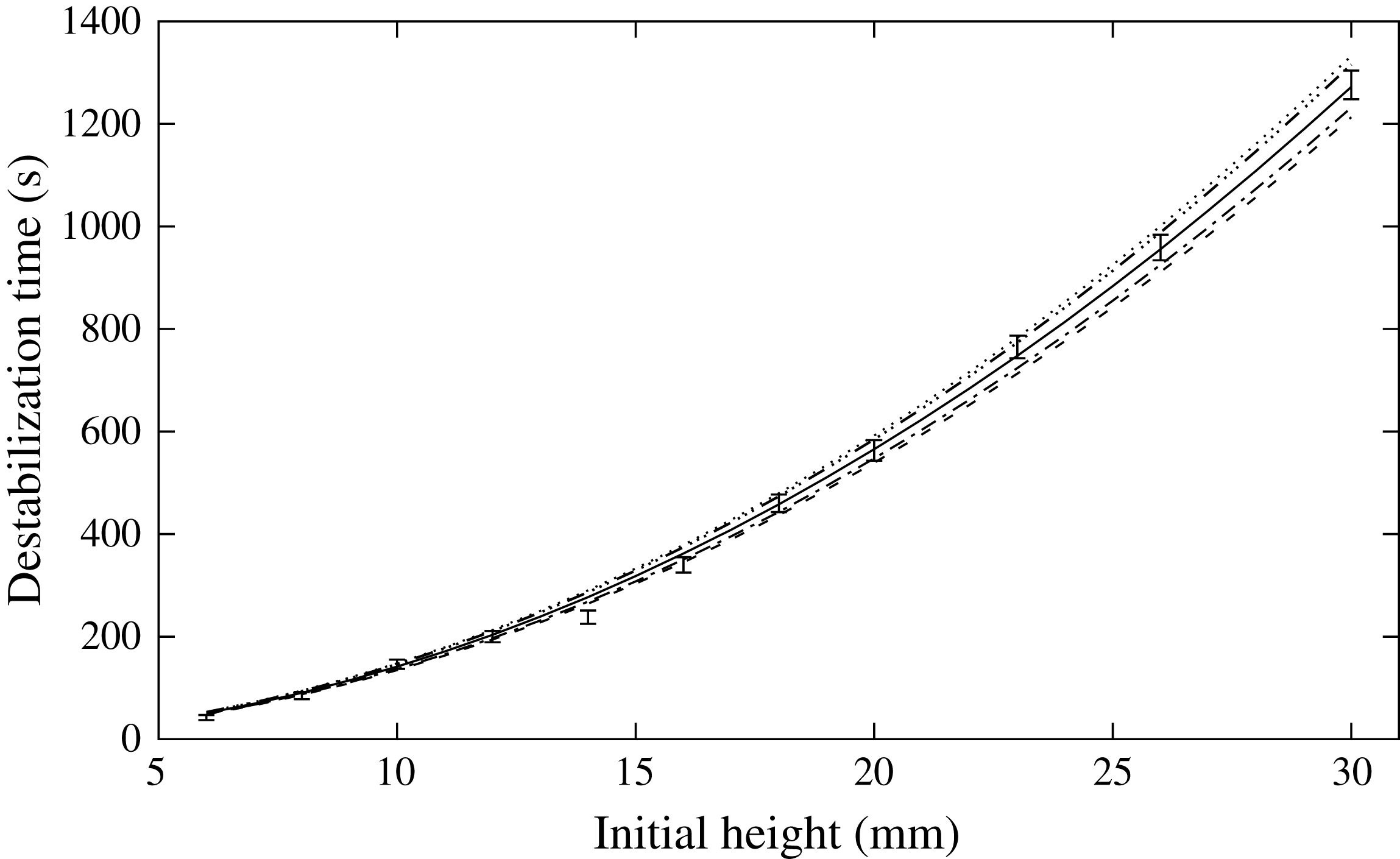
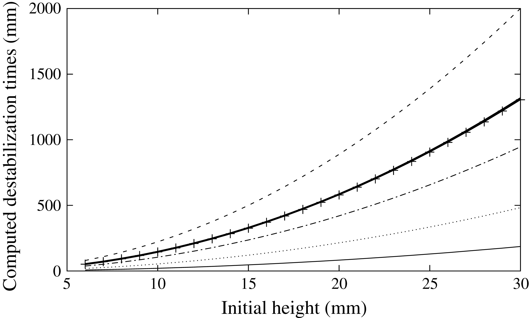
). The left-hand side of (4.5) can be analytically derived by direct quadrature formulas, to yield an equation in time. The zero of the obtained equation – which is too lengthy to be reproduced here – can then be numerically computed (the detailed analytic computation is really too lengthy and intricate to be reproduced in full length in the main text; instead, we provide the Maple code and corresponding output, which generated the obtained numerical values in the supplementary material). In figure 10 we plot the numerically obtained destabilization times
 $\unicode[STIX]{x1D70F}_{h}$
for this more realistic criterion (4.5), for the considered initial granular heights
 $h>5$
mm, and for
 $\unicode[STIX]{x1D6E5}=45~\text{K}$
. We also evaluate the sensitivity of the modelling to both parameters
 $\unicode[STIX]{x1D6E5}$
(initial temperature difference) and
 $\unicode[STIX]{x1D70C}_{g}^{c}-\unicode[STIX]{x1D70C}_{l}^{c}$
(initial grain/liquid density difference). Results obtained with a 1 K variation of the temperature difference
 $\unicode[STIX]{x1D6E5}$
and with a
 $\pm$
5 % variation of
 $\unicode[STIX]{x1D70C}_{g}^{c}-\unicode[STIX]{x1D70C}_{l}^{c}$
(by making
 $\unicode[STIX]{x1D70C}_{g}^{c}$
vary) are also plotted on figure 10. The quantitative accord between theoretical and experimental values is striking.
Destabilization time
 $\unicode[STIX]{x1D70F}_{h}$
(lines) for different values of the initial height
 $h$
as given by criterion (4.5). For the sensitivity analysis, we slightly vary the value of
 $\unicode[STIX]{x1D6E5}$
:
 $\unicode[STIX]{x1D6E5}=45~\text{K}$
(solid line, nominal value);
 $\unicode[STIX]{x1D6E5}=44~\text{K}$
(—
 $\cdots \,$
—);
 $\unicode[STIX]{x1D6E5}=46~\text{K}$
(—
 $\cdot$
—). The value of
 $\unicode[STIX]{x1D70C}_{l}^{c}$
(see text) is also varied such that the density initial difference
 $\unicode[STIX]{x1D70C}_{g}^{c}-\unicode[STIX]{x1D70C}_{l}^{c}$
is 5 % above or below the nominal density difference value of
 $7.1~\text{kg}~\text{m}^{-3}$
. The lower dashed line corresponds to 0.95
 $(\unicode[STIX]{x1D70C}_{g}^{c}-\unicode[STIX]{x1D70C}_{l}^{c})$
, while the upper dotted line corresponds to 1.05
 $(\unicode[STIX]{x1D70C}_{g}^{c}-\unicode[STIX]{x1D70C}_{l}^{c})$
.

It is worth noticing that such a simplified analytic modelling is now able to quantitatively predict the destabilization times for all sufficiently large initial layer heights.
4.3 Small
$h$
, incipient motion

The above subsection showed that the destabilization process is essentially due to thermal expansion of the whole layer, induced by the thermal conduction, when the initial layer is thick enough. However, for small thicknesses,
 $h\lesssim 5~\text{mm}$
, as shown in figure 8, a different regime of behaviour is observed.
We propose that in this case the incipient motion of the fluid is still triggered by the buoyancy directly induced by thermal heating through the very first layers at the bottom of the cell, but that the thermal boundary condition should no longer be assumed to be constant with time. Then, the settled spheres will be entrained by the fluid.
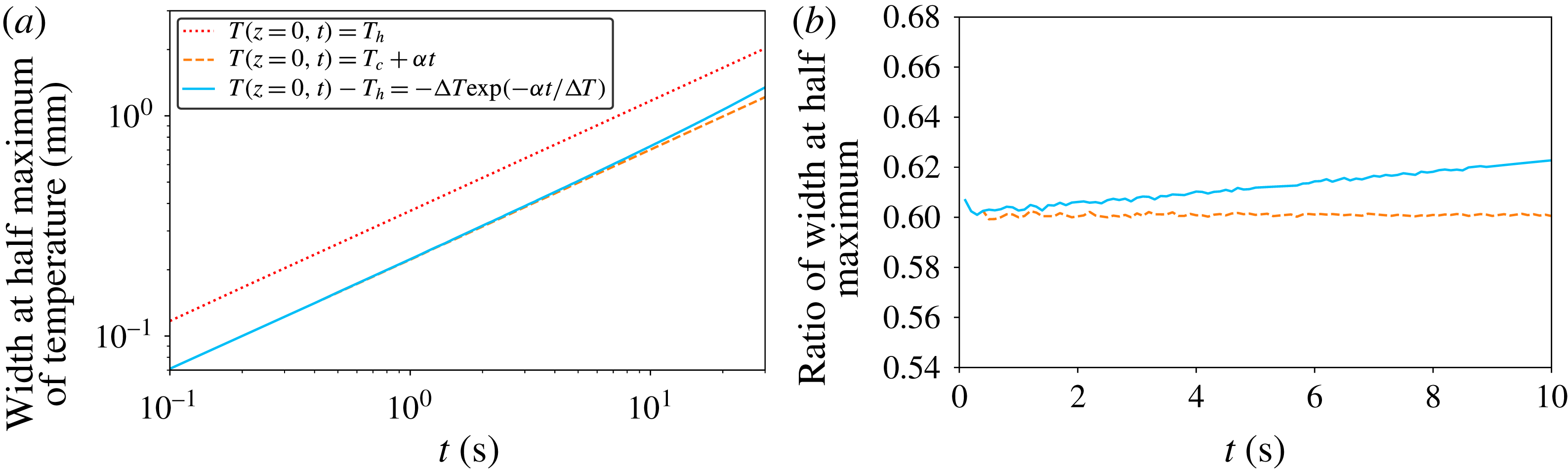
The key feature of the model is the time needed to raise significantly the temperature of the plate (and of the very first few millimetres above it). As seen in figure 3, the temperature increases almost linearly with time during the first instants. The plate temperature becomes constant after approximately 50 to 100 s, as already studied in Morize et al. (Reference Morize, Herbert and Sauret2017). Contrary to our approach for the thick layers, in which the bottom’s temperature was considered constant, we shall here include its evolution with time. We shall evaluate the force balance considering the column of fluid above the hot plate, which is heated only within a transient thermal boundary of thickness
 $\unicode[STIX]{x1D6FF}_{T}(t)$
. We assume moreover that the fluid can move only along the vertical axis due to the size ratio of
 $h$
to the width of the hot plate. The velocity is therefore constant with altitude
 $z$
. As the fluid rises due to buoyant effects, it exchanges momentum with the grains through viscous forces. We expect small velocities of the flow and assume that the Reynolds number associated with the transport of fluid inside the pores is low. Under this assumption, the superficial velocity (or the flux divided by the area of the plate)
 $q=\Vert \boldsymbol{q}\Vert$
of the fluid is given by Darcy’s law:
 $$\begin{eqnarray}\displaystyle \boldsymbol{q}=-\frac{\unicode[STIX]{x1D705}}{\unicode[STIX]{x1D707}}(\unicode[STIX]{x1D735}p-\unicode[STIX]{x1D70C}_{l}\boldsymbol{g}), & & \displaystyle\end{eqnarray}$$
with
 $p$
the local pressure,
 $\unicode[STIX]{x1D70C}_{l}$
the local density of the fluid and
 $\unicode[STIX]{x1D705}$
the coefficient of permeability of the granular layer (in
 $\text{m}^{2}$
). Equation (4.6) expresses the balance of viscous effects with weight and pressure gradient. We use a hydrostatic expression for pressure in the surrounding fluid. Integrating equation (4.6) from the bottom of the cell to the surface of the grains, we finally obtain the following equation:
 $$\begin{eqnarray}\displaystyle q & = & \displaystyle \frac{\unicode[STIX]{x1D705}}{\unicode[STIX]{x1D707}}\frac{1}{h}\left(\unicode[STIX]{x0394}p-\int _{z=0}^{h}\unicode[STIX]{x1D70C}_{l}g\,\text{d}z\right)=\frac{\unicode[STIX]{x1D705}}{\unicode[STIX]{x1D707}}\frac{1}{h}\left(\unicode[STIX]{x1D70C}_{l}^{c}gh-\int _{z=0}^{h}\unicode[STIX]{x1D70C}_{l}g\,\text{d}z\right)\nonumber\\ \displaystyle & = & \displaystyle \frac{\unicode[STIX]{x1D705}}{\unicode[STIX]{x1D707}h}\left(\int _{z=0}^{h}\unicode[STIX]{x1D70C}_{l}^{c}g\,\text{d}z-\int _{z=0}^{h}\unicode[STIX]{x1D70C}_{l}g\,\text{d}z\right)\nonumber\\ \displaystyle & = & \displaystyle -\frac{\unicode[STIX]{x1D705}}{\unicode[STIX]{x1D707}h}\left(\int _{z=0}^{\unicode[STIX]{x1D6FF}_{T}(t)}(\unicode[STIX]{x1D70C}_{l}(t,z)-\unicode[STIX]{x1D70C}_{l}^{c})g\,\text{d}z\right).\end{eqnarray}$$
Note that in the right-hand side, the integral above the thermal layer of thickness
 $\unicode[STIX]{x1D6FF}_{T}(t)$
cancels, because the densities are equal,
 $\unicode[STIX]{x1D70C}_{l}=\unicode[STIX]{x1D70C}_{l}^{c}$
. In the case of this one-dimensional thermal diffusion problem with a varying boundary condition, the temperature profile can be analytically computed, details are given in § A.4. However, further exact analytic computations are not possible, and we propose several assumptions in order to provide an approximate analytic solution. Since we are considering early times and small
 $z$
, we shall first assume that the temperature profile inside the thermal boundary layer of thickness
 $\unicode[STIX]{x1D6FF}_{T}(t)$
is accurately approximated by a triangular profile, with maximum temperature equal to the plate temperature.
Second, the temperature of the plate rises following an exponential relaxation that can be approximated as a linear increase at early time
 $t$
, with a constant rate
 $\unicode[STIX]{x1D6FC}$
. The coefficient
 $\unicode[STIX]{x1D6FC}$
is set by the experimental set-up and increases slightly with the thermal forcing. In the present case (
 $\unicode[STIX]{x1D6E5}=45$
K), its value
 $\unicode[STIX]{x1D6FC}=1.25~\text{K}~\text{s}^{-1}$
is measured from the slope of the experimental temperature curve at early times, as obtained by a fit of the linear temperature time evolution between
 $t=0$
s and 20 s. The average temperature
 $T(t)$
of the boundary layer is then given by:
 $$\begin{eqnarray}\displaystyle T(t)\approx (T(z=0,t)+T_{c})/2=T_{c}+\unicode[STIX]{x1D6FC}t/2. & & \displaystyle\end{eqnarray}$$
The third assumption is that the
 $\unicode[STIX]{x1D6FD}_{l}$
coefficient will be constant. We evaluate its value as an average both over the boundary layer
 $\unicode[STIX]{x1D6FF}_{T}$
and over the duration of linear increase of the temperature
 $(T_{h}-T_{c})/\unicode[STIX]{x1D6FC}$
leading to
 $\unicode[STIX]{x1D6FD}_{l}\approx 4.9\times 10^{-4}~\text{K}^{-1}$
. This approximation yields a very simple expression for
 $\unicode[STIX]{x1D70C}_{l}(z,t)\approx \bar{\unicode[STIX]{x1D70C}_{l}}=\unicode[STIX]{x1D70C}_{l}^{c}(1-\unicode[STIX]{x1D6FD}_{l}\unicode[STIX]{x1D6FC}t/2)$
. The next modelling step is to evaluate the thermal boundary layer thickness
 $\unicode[STIX]{x1D6FF}_{T}(t)$
. We adopt the classical scaling
 $\unicode[STIX]{x1D6FF}_{T}(t)=\unicode[STIX]{x1D6FE}\sqrt{4D_{th}t}$
, with
 $\unicode[STIX]{x1D6FE}$
a constant of the order of unity. Since the temperature is rising linearly with time, the thickness of the thermal boundary is approximately thinner, by a factor
 ${\sim}5/3$
(see § A.4, figure 18), than in the case of a fixed temperature. The velocity
 $q$
then increases with time until reaching the threshold value
 $q_{c}$
for the top layer of grains to be fluidized. Note that we can here only focus on the cold grains, because the lower layers are surrounded by lighter fluid and the buoyancy force is less efficient. The fluidization velocity
 $q_{c}$
can be estimated through Darcy’s law:
 $$\begin{eqnarray}\displaystyle q_{c}=\frac{\unicode[STIX]{x1D705}}{\unicode[STIX]{x1D707}}g(\unicode[STIX]{x1D70C}_{g}-\unicode[STIX]{x1D70C}_{l}^{c})\unicode[STIX]{x1D719}_{p}. & & \displaystyle\end{eqnarray}$$
For packed spheres of diameter
 $D$
, several semi-empirical relations can be found in the literature, yielding values of the same order (Rumpf & Gupte Reference Rumpf and Gupte1975; Kaviany Reference Kaviany1995). Following the Carman–Kozeny model (Kaviany Reference Kaviany1995), one can find for instance:
 $$\begin{eqnarray}\displaystyle \unicode[STIX]{x1D705}=\frac{D^{2}\unicode[STIX]{x1D700}^{3}}{180(1-\unicode[STIX]{x1D700})^{2}}. & & \displaystyle\end{eqnarray}$$
With the value
 $\unicode[STIX]{x1D700}=1-\unicode[STIX]{x1D719}_{p}=0.44$
, one finds
 $\unicode[STIX]{x1D705}\simeq 9.4\times 10^{-11}~\text{m}^{2}$
, with the bead diameter
 $D=250~\unicode[STIX]{x03BC}\text{m}$
, leading to a superficial fluidization velocity
 $q_{c}=2.9~\unicode[STIX]{x03BC}\text{m}~\text{s}^{-1}$
.
Combining (4.7) and (4.9) yields the following relation at the instability threshold:
 $$\begin{eqnarray}\displaystyle -\unicode[STIX]{x1D6FF}_{T}(\unicode[STIX]{x1D70F}_{h})(\bar{\unicode[STIX]{x1D70C}_{l}}(\unicode[STIX]{x1D70F}_{h})-\unicode[STIX]{x1D70C}_{l}^{c})=\unicode[STIX]{x1D719}_{p}(\unicode[STIX]{x1D70C}_{g}-\unicode[STIX]{x1D70C}_{l}^{c})h. & & \displaystyle\end{eqnarray}$$
With the approximations for the boundary layer thickness, equation (4.11) gives the following equation for the destabilization time:
 $$\begin{eqnarray}\displaystyle \unicode[STIX]{x1D6FE}\sqrt{4D_{th}}\unicode[STIX]{x1D70C}_{l}^{c}\unicode[STIX]{x1D6FD}_{l}\unicode[STIX]{x1D6FC}{\unicode[STIX]{x1D70F}_{h}}^{3/2}=2\unicode[STIX]{x1D719}_{p}(\unicode[STIX]{x1D70C}_{g}-\unicode[STIX]{x1D70C}_{l}^{c})h & & \displaystyle\end{eqnarray}$$
and hence the scaling:
 $$\begin{eqnarray}\displaystyle \unicode[STIX]{x1D70F}_{h}=\left[\frac{2\unicode[STIX]{x1D719}_{p}(\unicode[STIX]{x1D70C}_{g}-\unicode[STIX]{x1D70C}_{l}^{c})}{\unicode[STIX]{x1D6FE}\sqrt{4D_{th}}\unicode[STIX]{x1D70C}_{l}^{c}\unicode[STIX]{x1D6FD}_{l}\unicode[STIX]{x1D6FC}}\right]^{2/3}h^{2/3}. & & \displaystyle\end{eqnarray}$$
The value of
 $\unicode[STIX]{x1D70C}_{g}-\unicode[STIX]{x1D70C}_{l}^{c}$
can be taken as
 $\simeq 7~\text{kg}~\text{m}^{-3}$
and the other numerical values are
 $\unicode[STIX]{x1D719}_{p}=0.56$
,
 $\unicode[STIX]{x1D6FD}_{l}=4.9\times 10^{-4}~\text{K}^{-1}$
,
 $\unicode[STIX]{x1D6FC}=1.25~\text{K}~\text{s}^{-1}$
,
 $D_{th}=1.5\times 10^{-7}~\text{m}^{2}~\text{s}^{-1}$
,
 $\unicode[STIX]{x1D70C}_{l}^{c}=1053~\text{kg}~\text{m}^{-3}$
,
 $\unicode[STIX]{x1D6FE}=0.6$
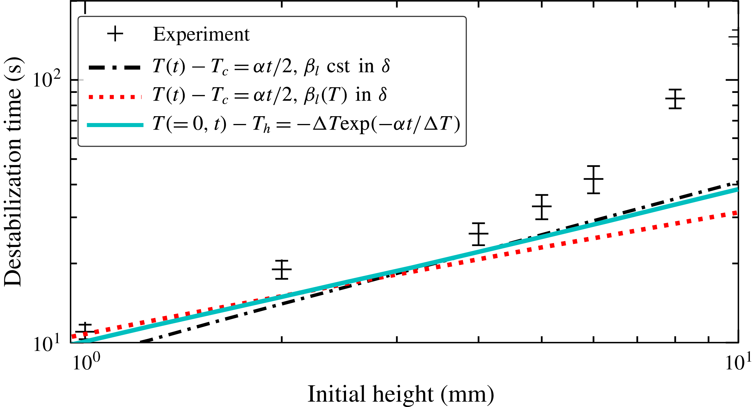
. Using the above formula, we obtain a first estimate for the destabilization times for small initial thicknesses, as shown in figure 11.


One should note that more refined modelling can be used that modify the previous scaling, but provide qualitatively the same order of magnitude of the found values (see § A.4). First, including the dependence of
 $\unicode[STIX]{x1D6FD}_{l}$
on the temperature brings a transition to another scaling
 $\unicode[STIX]{x1D70F}_{h}\propto h^{2/5}$
at larger values of
 $h$
(dotted line in figure 11); second, using the full expression of the analytic profile of temperature, a numerical integration is possible (solid line in figure 11). For these small thicknesses, measurements are more subject to local parameter variations (like
 $\unicode[STIX]{x1D719}$
) and uncertainties are expected to be larger than for higher values of
 $h$
. Since the proposed modelling is rather simple and one-dimensional, all the obtained curves can be considered to be in qualitative agreement with the measurements. However, the
 $2/3$
power law is only reproduced by the simplest model and the numerical computation. Using a simple argument, with no adjustable parameter, this fluidization model coupled with the transient thermal boundary layer expression provides values in quite fair agreement with experimental observations.
It is worth noticing that, after
 $t_{c}=\unicode[STIX]{x1D6E5}/\unicode[STIX]{x1D6FC}=36$
s, the temperature ramp reaches the plateau and therefore this scaling law stops being applicable. For thicknesses of the order of, or larger than,
 $\sqrt{4D_{th}\unicode[STIX]{x1D6E5}/\unicode[STIX]{x1D6FC}}\approx 4.5$
mm, the behaviour is then governed by a constant-temperature boundary condition, as presented in the previous section.
Two points of the modelling should be underlined. First, if the boundary layer remains inside the granular layer, this model provides almost the same equation than using the 1-D equivalent of (4.5), which is based on the average buoyancy of the bed, without the prefactor
 $(1-\unicode[STIX]{x1D719}_{p})$
in the left-hand side of (4.12). However, if this thermal boundary layer exceeds
 $h$
, our model still gives the same results, as shown below, unlike the 1-D form of (4.5). We think our approach is valid since the lighter fluid above would exert a depression when rising and would fully contribute to the driving force due to the small aspect ratio. For instance, at
 $h=1$
mm, the boundary layer is larger than
 $h$
by
 $500~\unicode[STIX]{x03BC}\text{m}$
, which is small compared to the width of the hot plate. Under the assumptions that this surface layer of heated fluid does not dissipate kinetic energy and that it is moving upward uniformly at the same velocity due to the small aspect ratio, the superficial velocity equation is:
 $$\begin{eqnarray}\displaystyle q & = & \displaystyle \frac{\unicode[STIX]{x1D705}}{\unicode[STIX]{x1D707}}\frac{1}{h}\left(\unicode[STIX]{x0394}p-\int _{z=0}^{h}\unicode[STIX]{x1D70C}_{l}g\,\text{d}z\right)\nonumber\\ \displaystyle & = & \displaystyle \frac{\unicode[STIX]{x1D705}}{\unicode[STIX]{x1D707}h}\left(\unicode[STIX]{x1D6FF}_{T}(t)\unicode[STIX]{x1D70C}_{l}^{c}g-\int _{h}^{\unicode[STIX]{x1D6FF}_{T}(t)}\unicode[STIX]{x1D70C}_{l}(z,t)g\,\text{d}z-\int _{z=0}^{h}\unicode[STIX]{x1D70C}_{l}g\,\text{d}z\right)\nonumber\\ \displaystyle & = & \displaystyle -\frac{\unicode[STIX]{x1D705}}{\unicode[STIX]{x1D707}h}\left(\int _{z=0}^{\unicode[STIX]{x1D6FF}_{T}(t)}(\unicode[STIX]{x1D70C}_{l}(t,z)-\unicode[STIX]{x1D70C}_{l}^{c})g\,\text{d}z\right).\end{eqnarray}$$
The driving force is still linked to
 $\unicode[STIX]{x1D6FF}_{T}$
, while the viscous resistance is still integrated over
 $h$
, which leads to the same equations (4.13).
The second point deals with the underestimate of the destabilization time by the 1-D model. We assumed that the velocity of the fluid was aligned with the vertical axis. When the thickness increases, the flux spreads more and more laterally, like for a water jet under a granular layer (Zoueshtiagh & Merlen Reference Zoueshtiagh and Merlen2007). Then the vertical velocity is lower and the destabilization time will be larger. Taking into account such an effect in the modelling would yield values closer to the experimental ones.
4.4 Expansion of the fluid
In this section, we model a second mechanism, related to the volume variation of the system bottom layers. As the basal layers are heated, just above the hot plate, their volume increases. Besides the aforementioned volume growth of grains with temperature, the fluid itself will be mechanically pushed upward, in addition to the buoyancy effect, by the thermal build-up of pressure. To evaluate this effect, instead of solving the full coupled equations for thermal diffusion and pressure inside a porous medium, as for instance in seismic studies (Andrews Reference Andrews2002), we shall directly simplify and model the considered phenomenon. More specifically, we consider the conservation of the mass of fluid inside a growing vertical column of height
 $h^{\ast }$
above the hot plate and inside the granular layer, and we estimate the fluid velocity at the surface of the granular bed by splitting the column in two parts: the heated part and the cold part, separated by a moving boundary. The thickness
 $\unicode[STIX]{x1D6FF}_{T}$
of the thermal boundary layer is assumed to be given only by the static thermal problem, as before. Using the same notation as in the previous section, this layer thickness
 $\unicode[STIX]{x1D6FF}_{T}$
is assumed to be at the boundary layer’s average temperature. Its fluid density is lower while the remaining layer (of height
 $h^{\ast }-\unicode[STIX]{x1D6FF}_{T}(t)$
) maintains its density unchanged. The mass conservation equation is therefore given by the following equation:
 $$\begin{eqnarray}\displaystyle & \displaystyle 0=(1-\unicode[STIX]{x1D719}_{p})\frac{\text{d}}{\text{d}t}\left[\int _{0}^{h^{\ast }}\unicode[STIX]{x1D70C}_{l}(z,t)\,\text{d}z\right], & \displaystyle\end{eqnarray}$$
 $$\begin{eqnarray}\displaystyle & \displaystyle 0=\frac{\text{d}}{\text{d}t}\left[\int _{\unicode[STIX]{x1D6FF}_{T}}^{h^{\ast }}\unicode[STIX]{x1D70C}_{l}(z,t)\,\text{d}z+\int _{0}^{\unicode[STIX]{x1D6FF}_{T}}\unicode[STIX]{x1D70C}_{l}(z,t)\,\text{d}z\right], & \displaystyle\end{eqnarray}$$
 $$\begin{eqnarray}\displaystyle & \displaystyle 0=\unicode[STIX]{x1D70C}_{l}^{c}\frac{\text{d}h^{\ast }}{\text{d}t}+\frac{\text{d}\unicode[STIX]{x1D6FF}_{T}}{\text{d}t}(\unicode[STIX]{x1D70C}_{l}(\unicode[STIX]{x1D6FF}_{T}^{-},t)-\unicode[STIX]{x1D70C}_{l}(\unicode[STIX]{x1D6FF}_{T}^{+},t)+\int _{0}^{\unicode[STIX]{x1D6FF}_{T}}\frac{\text{d}\unicode[STIX]{x1D70C}_{l}(z,t)}{\text{d}t}\,\text{d}z. & \displaystyle\end{eqnarray}$$
Assuming the same expression than before for
 $\unicode[STIX]{x1D6FF}_{T}(t)$
, and that
 $\bar{\unicode[STIX]{x1D70C}_{l}}\approx \unicode[STIX]{x1D70C}_{l}^{c}(1-\unicode[STIX]{x1D6FD}_{l}\unicode[STIX]{x1D6FC}t/2)$
, one can obtain the expression of the rising velocity
 $v_{-}^{r}$
as the time derivative of
 $h^{\ast }$
, for early times
 $t<t_{c}$
:
 $$\begin{eqnarray}\displaystyle v_{-}^{r} & = & \displaystyle +\frac{\text{d}\unicode[STIX]{x1D6FF}_{T}}{\text{d}t}\left(1-\left(1-\unicode[STIX]{x1D6FD}_{l}\unicode[STIX]{x1D6FC}\frac{t}{2}\right)\right)+\int _{0}^{\unicode[STIX]{x1D6FF}_{T}}\unicode[STIX]{x1D6FD}_{l}\unicode[STIX]{x1D6FC}\frac{1}{2}\,\text{d}z\end{eqnarray}$$
 $$\begin{eqnarray}\displaystyle & = & \displaystyle \frac{3}{4}\unicode[STIX]{x1D6FE}\sqrt{4D_{th}t}\unicode[STIX]{x1D6FD}_{l}\unicode[STIX]{x1D6FC}\quad \text{for}~t<t_{c}.\end{eqnarray}$$
For the times
 $t>t_{c}$
, we assume that the temperature of the plate reaches
 $T_{h}$
and that the thickness of the boundary layer is described by the classical expression without the
 $\unicode[STIX]{x1D6FE}$
, to obtain the asymptotic behaviour, taking the average value of
 $\unicode[STIX]{x1D70C}_{l}$
:
 $$\begin{eqnarray}\displaystyle v_{+}^{r} & = & \displaystyle -\frac{\text{d}\unicode[STIX]{x1D6FF}_{T}}{\text{d}t}\left(\frac{\bar{\unicode[STIX]{x1D70C}_{l}}}{\unicode[STIX]{x1D70C}_{l}^{c}}-1\right)-\int _{0}^{\unicode[STIX]{x1D6FF}_{T}}0\,\text{d}z\end{eqnarray}$$
 $$\begin{eqnarray}\displaystyle & = & \displaystyle \frac{1}{2}\sqrt{\frac{4D_{th}}{t}}\left(1-\frac{\bar{\unicode[STIX]{x1D70C}_{l}}}{\unicode[STIX]{x1D70C}_{l}^{c}}\right)\quad \text{for}~t>t_{c},\end{eqnarray}$$
where
 $\bar{\unicode[STIX]{x1D70C}_{l}}=(\unicode[STIX]{x1D70C}_{l}(T_{h})+\unicode[STIX]{x1D70C}_{l}^{c})/2$
.
Since
 $v_{-}^{r}$
increases with time while
 $v_{+}^{r}(t)$
decreases, the maximal rising velocity is reached at the transition between the two regimes (at
 $t=t_{c}$
), to yield
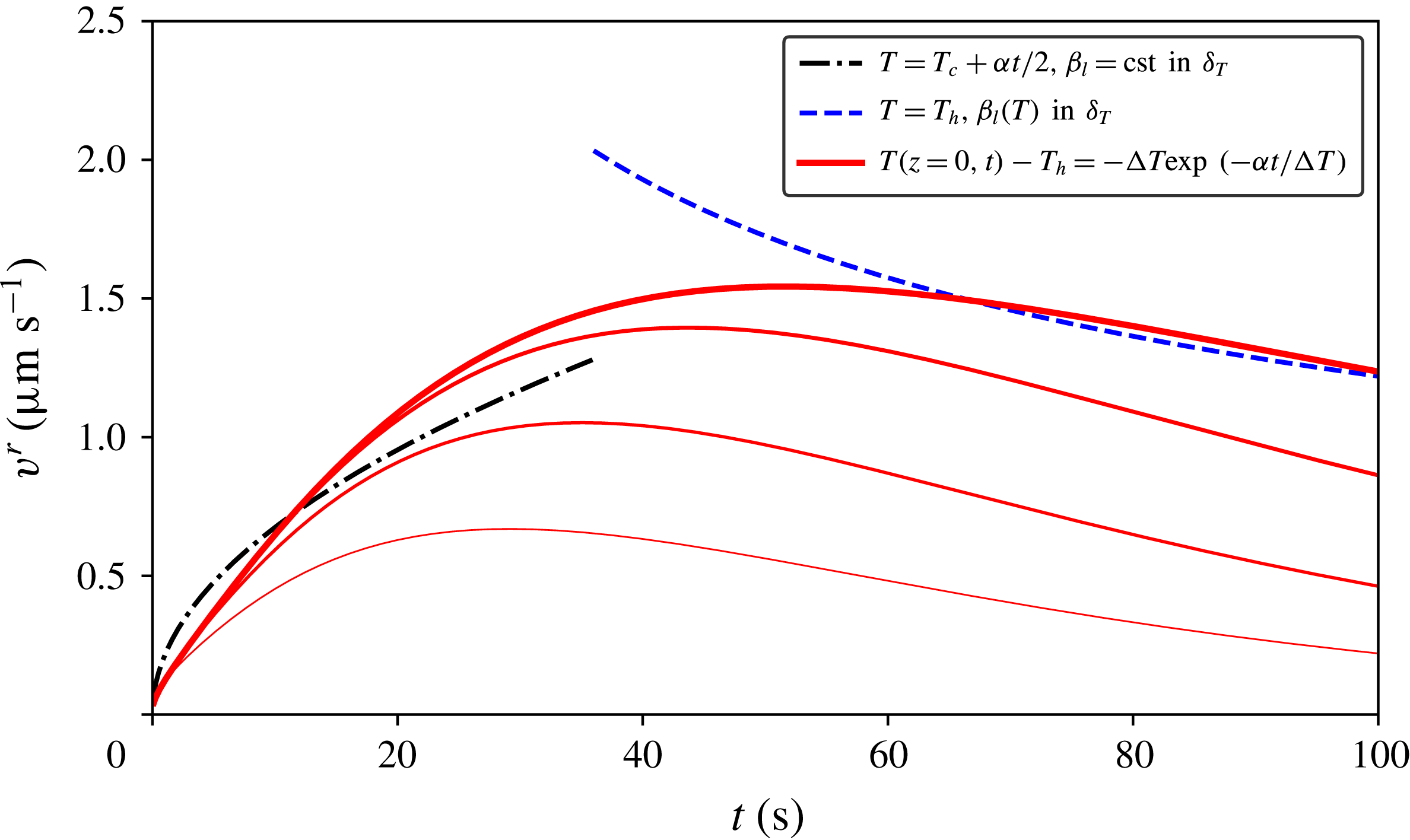
 $v_{max}^{r}\simeq 1~\unicode[STIX]{x03BC}\text{m}~\text{s}^{-1}$
as shown in figure 12. The obtained value for this maximal velocity is therefore too weak to trigger the plume emission. This justifies the main mechanism of our approach in the previous section. However, a correction of the destabilization time can be made, because this rising velocity increases the velocity due to buoyancy, leading to a slower time. Note that these expressions consider the top of the thermal boundary layer which can exceed the thickness
 $h$
. Therefore at the surface of the granular layer, the velocity could be smaller. To estimate it, we use the full expression of the thermal boundary layer given in the appendix A (A 10). The rising velocities
 $v^{r}$
from the last equations and the results of the numerical integration for different heights are plotted in figure 12. It is worth noting that we do not solve the full advection–diffusion equation, but instead, we use (4.15) and the computed thermal boundary layer. Nevertheless, since the relative change of density is at most 6 %, the precision of our model is quite fair. Finally, for thicker layers, the flow is able to spread laterally, leading the intensity to decrease locally as reported for ascending water jets in porous media (Rigord et al.
Reference Rigord, Guarino, Vidal and Géminard2005; Mena et al.
Reference Mena, Luu, Cuéllar, Philippe and Sinclair Curtis2017). Such vertical velocity can therefore decrease the sedimentation rate of the particles. However, this model is not accurate enough to capture the amplitude of the slowing down observed for larger thicknesses.
Rising velocity due to the dilatancy of the heated fluid. The dark dashed and dotted lines correspond to the simplified modelling, equations (4.21) and (4.19). The solid lines used the numerical profile (A 10), for respectively
 $h=1$
mm, 2 mm, 4 mm, and
 $\infty$
(from thinner to thicker lines).

4.5 Liquefaction and repacking front propagation
Let us now focus on the early transient behaviour of the granular bed surface. For each value of
 $h$
within the range 8–30 mm, we study the time evolution of the volume variations
 $\unicode[STIX]{x0394}S$
, as already shown in figure 7. After the slight initial growth, the curves decrease, for all
 $h$
values, following almost parallel straight lines. This behaviour is interpreted as granular layer liquefaction after an initial perturbation (Pouliquen, Belzons & Nicolas Reference Pouliquen, Belzons and Nicolas2003). The perturbation can be either the initial fluid motion or the volume increase of the heated grains at the bottom, that then changes contacts and force networks (Coulais, Seguin & Dauchot Reference Coulais, Seguin and Dauchot2014). Since initially the settled spheres’ arrangement is characterized by the volume fraction of a random loose packing, the initial perturbation is enough to trigger a small motion of the grains. The liquefaction is then immediately followed by granular bed sedimentation (Mutlu Sumer et al.
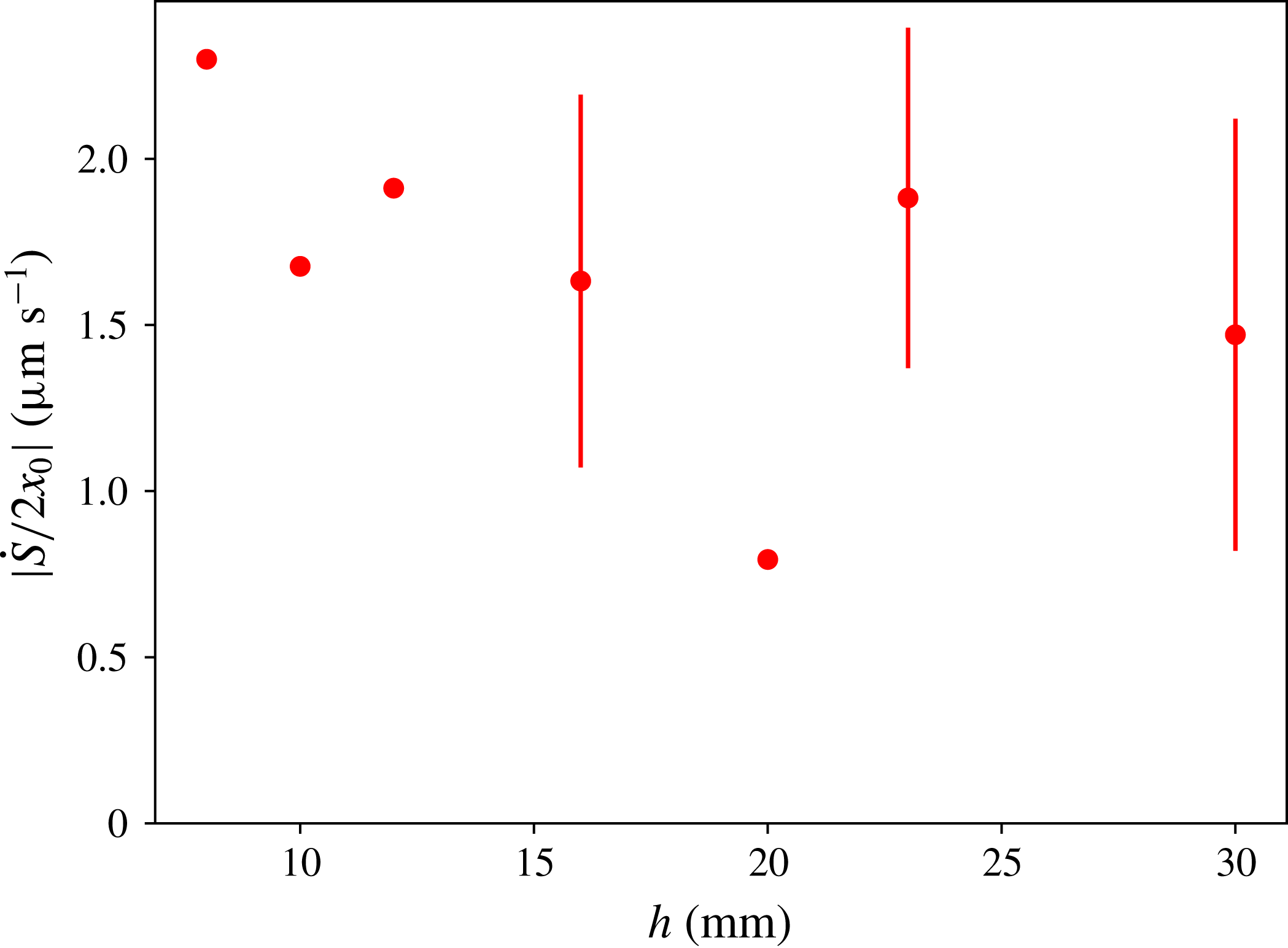
Reference Mutlu Sumer, Hatipoglu, Fredsøe and Kaan Sumer2006). When varying
 $h$
, the values of the
 $\unicode[STIX]{x0394}S(t)$
slopes were found respectively to be
 ${\dot{S}}=100$
, 128, 54, 111, 130, 114,
 $159\times -10^{-3}~\text{mm}^{2}~\text{s}^{-1}$
, for
 $h=30$
, 23, 20, 16, 12, 10 and 8 mm. We expect the average velocity to be close to the fluidization velocity value computed in the previous section, i.e.
 $q_{c}=2.9~\unicode[STIX]{x03BC}\text{m}~\text{s}^{-1}$
. By dividing
 ${\dot{S}}$
by the plate width
 $2x_{0}$
, we obtain the average velocity of the bed surface, as plotted, for varying
 $h$
, in figure 13. The values of the velocities are in the range of the fluidization velocity, but smaller. We interpret these smaller values by the fact that the fluid is already moving upward due to the thermal forcing, even before the destabilization, as shown in the previous sections.
Average sedimentation velocity of the granular bed after the initial disturbance as a function of height
 $h$
computed over the width
 $2x_{0}$
. The error bars correspond to the velocity computed over varying width, from
 $2x_{0}$
to
 $L$
, and centred around the middle of the hot plate.

We also observed that the granular bed upper surface did not remain flat during the fluidization process, and we were able to measure upward and downward motion all along the free surface above the hot plate. Separating those two components in figure 7, we observed that the areas that were still sedimenting had the same average velocity. Moreover, our precise measurements also showed interface fluctuations of up to
 $250~\unicode[STIX]{x03BC}\text{m}~\text{s}^{-1}$
. These interface fluctuations can be linked to the velocity fluctuations observed in settling suspensions (Guazzelli & Hinch Reference Guazzelli and Hinch2011). They are reported to be of the order of the settling velocity and here
 $250~\unicode[STIX]{x03BC}\text{m}~\text{s}^{-1}$
corresponds to the Stokes’ velocity of one of our spheres.
This local reorganization of the layer from a loose random packing (with
 $\unicode[STIX]{x1D719}_{0}=0.56$
) to a more closely packed granular bed, with typically
 $\unicode[STIX]{x1D719}=\unicode[STIX]{x1D719}_{1}\simeq 0.60{-}0.64$
from the literature, has the net effect of decreasing the apparent layer volume while the interstitial liquid is expelled from the bed. During this process, a compaction front should arise from the cell bottom (Pouliquen et al.
Reference Pouliquen, Belzons and Nicolas2003; Mutlu Sumer et al.
Reference Mutlu Sumer, Hatipoglu, Fredsøe and Kaan Sumer2006). From mass conservation of the solid, one can derive the associated celerity
 $c$
of this compaction front propagation, that reads:
 $$\begin{eqnarray}\displaystyle c=\frac{1}{1-\unicode[STIX]{x1D719}_{1}/\unicode[STIX]{x1D719}_{0}}\frac{{\dot{S}}}{2x_{0}}. & & \displaystyle\end{eqnarray}$$
For typical values of
 $\unicode[STIX]{x1D719}_{1}$
(
 $\unicode[STIX]{x1D719}_{1}\simeq 0.60$
–0.64) and
 ${\dot{S}}/2x_{0}$
(
 ${\approx}1.5$
–
 $2~\unicode[STIX]{x03BC}\text{m}~\text{s}^{-1}$
, see figure 13), equation (4.22) yields
 $c\sim 10$
–
 $25~\unicode[STIX]{x03BC}\text{m}~\text{s}^{-1}$
. The estimated value for
 $c$
is quite in line with the value of the compaction front velocity reported in Kiesgen de Richter et al. (Reference Kiesgen de Richter, Hanotin, Marchal, Leclerc, Demeurie and Louvet2015):
 $c\sim 20~\unicode[STIX]{x03BC}\text{m}~\text{s}^{-1}$
for the considered case of vibration-induced reorganization. We note that the final state of the sedimentation is not reached, comparing the destabilization time to
 $h/c$
. The destabilization time is always smaller that the time required to settle the whole granular column after fluidization in our experiments. The limit thickness
 $h_{s}$
can be estimated with a similar strategy as before, identifying
 $h_{s}/c$
and
 $\unicode[STIX]{x1D70F}_{h}$
:
 $h_{s}\approx \sqrt{4D_{th}/c}(1-\unicode[STIX]{x1D719}_{p})\unicode[STIX]{x1D70C}_{l}^{c}\unicode[STIX]{x1D6FD}_{l}\unicode[STIX]{x1D6E5}/(\unicode[STIX]{x1D719}_{p}(\unicode[STIX]{x1D70C}_{g}-\unicode[STIX]{x1D70C}_{l}^{c}))\approx 45~\text{mm}$
, where both times are of the order of
 $2\times 10^{3}$
s. This last estimate confirms that the granular layer remains in a fragile state before the destabilization time and does not form a densely packed sediment that would be difficult to fluidize locally. Indeed, in addition to the weight of the grains, the thermal forcing would have to overcome the Reynolds’ dilatancy and the granular friction on all the vertical boundaries. This supports our assumption neglecting the lateral granular friction along the column of grains, for plume triggering. It would be interesting to study densely compacted beds (like e.g. densely packed geophysical sediments), where a decrease of the volume fraction should precede the arrival of the plume. As mentioned above, for even larger thicknesses of bed, this dilatancy may also appear if the recompaction front reaches the top surface before the plume appears.
Finally, we would like to comment on the fluid flow through the porous granular medium just above the hot plate, after the destabilization occurs. When the plume is triggered, the fluid rises together with the grains. Hence, new fresh fluid must fill the lower part of the bed. We have not yet measured nor modelled this flow; however, figure 14 evidences the phenomenon. Observation of the layer’s bulk after the plume’s emission makes apparent a large-scale fluidization process, i.e. the grain and liquid mixture in the fluidized pocket has a fluid-like behaviour, foregoing the cavity (filled almost only with liquid) formation shown in figure 5. We think that the secondary flow, which we cannot observe directly with our lateral camera, is already at work long before the plume emission. The hole formation shares similarities with experiments where an ascending liquid is directly injected below the granular layer (Rigord et al. Reference Rigord, Guarino, Vidal and Géminard2005; Zoueshtiagh & Merlen Reference Zoueshtiagh and Merlen2007; Philippe & Badiane Reference Philippe and Badiane2013). However, a focusing effect due to internal recirculation, that is not present when fluid is injected from the bottom, may enhance the fluid’s vertical motion.
Observations of the bulk of the granular layer at times
 $t>\unicode[STIX]{x1D70F}_{h}$
((a–c) 220, 240 and 260 s after destabilization), for
 $h=30$
mm. The cavity growth occurs mainly in the vertical direction.

5 Concluding remarks, perspectives
In the present paper, we experimentally and analytically analysed thermally driven destabilization of an immersed granular layer, made up of spherical, mono-disperse,
 $250~\unicode[STIX]{x03BC}\text{m}$
in diameter, polystyrene spheres, surrounded by salt water. The experimental apparatus consisted of a rectangular tank in which the initially quiescent granular layer was heated from below, while the temperature above was maintained constant. The initial density difference (at low temperature) between polystyrene and the surrounding aqueous 6.5 % CaCl
 $_{2}$
salt mixture is approximately
 $7~\text{kg}~\text{m}^{-3}$
. For sufficiently large values of the initial granular layer height
 $h$
, the power law scaling for the conduction-driven destabilization time
 $\unicode[STIX]{x1D70F}_{h}\propto h^{2}$
, is accurately captured by the present modelling. Despite the finite length geometry, preliminary purely conductive numerical computations showed that three-dimensional conductive situations can be fairly well approximated using 1-D analytic solutions for each radial direction (except for the directions very close to the zero-flux bottom boundary surface, as shown in appendix A). Considering a temperature-dependent coefficient of thermal expansion
 $\unicode[STIX]{x1D6FD}_{m}$
for the grain/water mixture as well as a 3-D hemispherical shape for the heated granular layer volume, yields a simple analytically/numerically tractable criterion for destabilization times, with no adjustable parameter. Numerical solution of the proposed criterion leads to striking quantitative agreement with experimental results, when the initial height
 $h$
is large enough. For smaller values of
 $h$
(
 $h\lesssim \unicode[STIX]{x1D6FF}_{T}(\unicode[STIX]{x1D6E5}/\unicode[STIX]{x1D6FC})$
), the phenomenon is driven by the transient increase of temperature: the settled spheres’ motion is triggered by Darcy flow through the granular layer, driven by the thermal heating of the fluid inside the lower part of the granular bed.
Introducing the time-dependent boundary condition, the proposed simple modelling allowed us to capture the
 $2/3$
power scaling for the destabilization time at small
 $h$
. Moreover, with no fitting parameter, a quite fair agreement is obtained between the numerical values and the experimental results, showing the transition between the steady and transient regimes of conduction. It is worth noting that this agreement holds even if several secondary flows, which we have pointed out, are not taken into account.
The present paper focused on the early evolution of the granular layer, i.e. up to the layer thermal destabilization and jet formation. The subsequently observed phenomena, namely the development of the jet, its structure and topology (including the formation of a mushroom cloud and the presence/absence of Kelvin–Helmholtz and Rayleigh–Taylor instabilities) the cavitation processes in the layer bulk, the re-sedimentation of the ejected particles on the layer upper boundary as well as the angle of avalanche evolution (coming from the avalanching process following the buoyant flow), will be analysed elsewhere.
The present analysis also paves the way to more elaborate multi-dimensional computations. In the first place, one can think of quite detailed (and complex) modelling simulations, based for instance on a discrete element method (DEM) strategy, e.g. as first introduced in Cundall & Strack (Reference Cundall and Strack1979). In this approach, the particles of the granular flow are considered as rigid or slightly deformable solids with point interactions. By solving the individual laws of motion for each solid particle, namely translational and angular momentum, the DEM approach is able to compute the motion of each particle at the micro level. Beyond the inclusion of a sufficient number of individual particles – here the real number of particles is
 ${\sim}10^{6}$
–
 $10^{7}$
, depending on
 $h$
, but a few
 $10^{5}$
may be sufficient to capture the main features – and the necessary coupling with a computational fluid dynamics (CFD) solver (Kloss et al.
Reference Kloss, Goniva, Hager, Amberger and Pirker2012), the approach also requires a specific modelling for particle contacts, see for instance Stroh et al. (Reference Stroh, Alobaid, Hasenzahl, Hilz, Strohle and Epple2016), Khanal & Jayasundara (Reference Khanal and Jayasundara2014), Maréchal (Reference Maréchal2016). For DEM-like, i.e. at the particle level, strategies, the main limitation remains the numerical cost, both in terms of processing time (i.e. CPU or central processing unit time) and memory (Alobaid, Baraki & Epple Reference Alobaid, Baraki and Epple2014), even if the wall-clock (real) time can be markedly leveraged, e.g. using parallel implementation (Amritkar, Deb & Tafti Reference Amritkar, Deb and Tafti2014) and/or GPU (graphic processing unit) (Jajcevic et al.
Reference Jajcevic, Siegmann, Radeke and Khinast2013).
An alternative, much less expensive, approach may be numerical modelling of two-phase continuous media, considering the granular mixture as a non-Newtonian yield stress fluid, the effective viscosity of which may depend on local shear rate, local pressure exerted on the particles and local packing density (Note that a DEM-CFD approach may help in developing constitutive models for continuum-based computations of larger-scale processes, bridging the gap between small (micro) scale – at the so-called ‘subgrid scale’ – and large (macro) scale, see e.g. Guo & Sinclair Curtis (Reference Guo and Sinclair Curtis2015).). Due to its much lighter computational cost, this approach is currently used in many engineering applications, but of course suffers from its lack of generality. Specific issues, e.g. the numerical implementation of adapted efficient algorithms, the coupling with heat transfer, and the regularization problem for vanishing shear rate, were identified and gave birth to a vast literature (see e.g. the recent review by Saramito & Wachs (Reference Saramito and Wachs2017), a comparison of different modelling approaches (Fraggedakis, Dimakopoulos & Tsamopoulos Reference Fraggedakis, Dimakopoulos and Tsamopoulos2016), or the more specific simulation of a thermal plume (Karimfazli, Frigaard & Wachs Reference Karimfazli, Frigaard and Wachs2016), a situation which resembles ours). Another recent approach is more specifically dedicated to dense granular flows. Following the MiDi research group (GDR MiDi 2004), the
 $\unicode[STIX]{x1D707}(I)$
-rheology approach proposed a constitutive law for dry granular flows (Jop, Forterre & Pouliquen Reference Jop, Forterre and Pouliquen2006). The strategy was also implemented for multi-dimensional simulations (Lagrée, Staron & Popinet Reference Lagrée, Staron and Popinet2011; Chauchat & Médale Reference Chauchat and Médale2014), still in the dry case, and extended to submarine (Cassar, Nicolas & Pouliquen Reference Cassar, Nicolas and Pouliquen2005) and wet saturated situations (Boyer, Guazzelli & Pouliquen Reference Boyer, Guazzelli and Pouliquen2011). Despite many significant improvements, as witnessed by the above-cited literature, both modelling and computational issues still remain, even if promising studies of localized fluidization cavities in granular beds can be found (e.g. Ngoma et al.
Reference Ngoma, Philippe, Bonelli, Delenne, Radjai, Soga, Kumar, Biscontin and Kuo2015).
To conclude, as emphasized in the recent work by Blumenfeld et al. (Reference Blumenfeld, Amitai, Jordan and Hihinashvili2016), the continuous media approach still requires sufficiently specific and accurate equations of state. To this aim, and in order to explore the diversity of behaviours that dense suspensions exhibit through hydro-thermo-mechanical coupling, further experimental work is also required.
Acknowledgements
The authors would like to thank S. Herbert and E. Kaminski for fruitful discussions and G. Ducournau for help in the experimental work. This work was granted access to the HPC resources of CRIANN (Centre Régional Informatique et d’Applications Numériques de Normandie), yielding the 3-D computations shown in the appendix, under the allocation 2008013. One of the authors (EH) acknowledges support of the French Agence Nationale de la Recherche (ANR), through the program STABINGRAM.
Supplementary movie and material
Supplementary movie and material are available at https://doi.org/10.1017/jfm.2018.141.
Appendix A
A.1 Approximate time-dependent temperature profile
As mentioned in the main text, the time-dependent temperature profile in the bed may in principle be computed analytically using suitable heat equation Green kernels, compatible with the boundary conditions. However, obtaining the closed form solution is not only tedious but yields intricate expressions, difficult – if not impossible – to handle analytically. In this subsection, in a more practical approach, we shall demonstrate that an approximate, but still quite accurate, expression can be derived thanks to 3-D heat conduction simulations. Making use of the popular OpenFoam solver suite, we numerically computed the temperature profile in the tank. We plot on figure 15 the profiles of the reduced temperature
 $\unicode[STIX]{x1D703}=(T(r,t)-T_{h})/(T_{c}-T_{h})$
with respect to the Fourier number (based on the radius
 $r$
)
 $u=r/2\sqrt{D_{th}t}$
for time
 $t=140$
s, respectively for the vertical axis and two radial axes, as shown in figure 16. Except for the large-angle radial axis (close to the lower boundary), the suggested 1-D-like relation
 $\unicode[STIX]{x1D703}=\text{erf}(u)$
is recovered.
Reduced temperature
 $(T(r,t)-T_{h})/(T_{c}-T_{h})$
as a function of radius-based Fourier number
 $r/2\sqrt{D_{th}t}$
for time
 $t=140$
s and for the three lines represented in figure 16. The thick solid line represents the vertical axis profile, while the dashed and the dotted-dashed lines are respectively the low-angle diagonal axis profile and the
 $\text{erf}(u)$
solution. As expected, while the vertical axis and the low-angle diagonal quite accurately follow the
 $\text{erf}(u)$
profile, the high-angle diagonal profile, encompassing a region close to the bottom colder plate (the non-metallic walls with Neumann boundary condition, see the caption of figure 16) markedly departs from the
 $\text{erf}(u)$
profile.

Vertical axis, low-angle and high-angle diagonal axes which profiles are drawn on figure 15. The boundary conditions are fixed temperature
 $T_{h}$
on the lower metallic plate (as delimited in the above sketch), fixed temperature
 $T_{c}$
on the above wall, homogeneous Neumann condition on the side walls and on the horizontal lower non-metallic walls.

A.2 Comparison of the different modellings for the destabilization time
$\unicode[STIX]{x1D70F}_{h}$

In this subsection, we compare the different criteria to quantitatively capture the destabilization times for large
 $h$
. Note that all the proposed criteria are based on a purely conductive modelling and will hence predict the correct scaling
 $\unicode[STIX]{x1D70F}\propto h^{2}$
. The discussion will therefore compare the numerical values for the prefactor. We start with the proposed three-dimensional criterion, referred to as C3DaTb in the following, which is the criterion given by (4.5) and reported in the figure 8 of the main text:
 $$\begin{eqnarray}\displaystyle \int _{r=0}^{r=h}(\bar{\unicode[STIX]{x1D70C}}-\unicode[STIX]{x1D70C}_{l}^{c})r^{2}\,\text{d}r=0. & & \displaystyle\end{eqnarray}$$
We also evaluate the same criterion in its one-dimensional version (referred to as C1DaTb in the following), which is similar to the criterion proposed in Morize et al. (Reference Morize, Herbert and Sauret2017):
 $$\begin{eqnarray}\displaystyle \int _{z=0}^{z=h}(\bar{\unicode[STIX]{x1D70C}}-\unicode[STIX]{x1D70C}_{l}^{c})\,\text{d}z=0. & & \displaystyle\end{eqnarray}$$
Note that in all the considered cases the temperature profile is given by (4.3) of the main text (with
 $z\equiv r$
for the 3-D case). In order to change a unique parameter (here the number of dimensions), the dilatation coefficient for water is taken in both equations (A 1) and (A 2) as depending on the local temperature, as explained in the main text:
 $$\begin{eqnarray}\displaystyle \unicode[STIX]{x1D6FD}_{l}=aT-b. & & \displaystyle\end{eqnarray}$$
We also compared the results obtained with criteria (A 1) and (A 2) by using a parameterized modelling for the one-dimensional criterion (A 2). We assumed that the dilatation coefficient
 $\unicode[STIX]{x1D6FD}_{l}$
for the salt water is taken at a fixed given temperature
 $T_{0}$
and is no more variable with the temperature:
 $\unicode[STIX]{x1D6FD}_{l}=aT_{0}-b=\text{constant}$
. The parameter
 $T_{0}$
is varied and the considered values are respectively
 $T_{0}=290$
, 292, 294 and 300 K, yielding to one-dimensional type criteria, respectively referred to as C1D290, C1D292, C1D294, C1D300. The numerical resolution of the different criteria C3DaTb, C1DaTb, C1D290, C1D292, C1D294, C1D300 yields different destabilization times, which are represented in figure 17.
Computed destabilization times using respectively criteria C3DaTb (thick solid line), C1DaTb (thin solid line), C1D290 (dashed line), C1D292 (large
 $+$
), C1D294 (dotted-dashed line), C1D300 (dotted line).

The quantitative values obtained with C1DaTb are in clear disagreement (by a factor
 $\simeq 1/7$
) with the present proposed 3-D criterion (see (4.5) and figure 8 in the main text). Note that the criterion C1D292 allows to recover the correct quantitative values, by varying the
 $T_{0}$
parameter. However, the results are very sensitive to the value of
 $T_{0}$
, as shown by the curves obtained by the other criteria C1D290 (
 $\times 1.5$
), C1D294 (
 $\times 0.72$
) and C1D300 (
 $\times 0.37$
).
A.3 A possible link with buoyancy-induced volcanic mush destabilization
In this subsection, we suggest how the present study can be connected to a regime of magmatic eruptions triggered by buoyancy, as identified in Degruyter & Huber (Reference Degruyter and Huber2014). The mush, i.e. the mixture of ‘liquid’ magma and solid crystals, of density
 $\unicode[STIX]{x1D70C}_{M}$
, lies beneath liquid magma, of density
 $\unicode[STIX]{x1D70C}_{l}$
initially lower than
 $\unicode[STIX]{x1D70C}_{M}$
. The mush can be destabilized (or not) by several mechanisms: mass injection, second boiling, buoyancy. In Degruyter & Huber (Reference Degruyter and Huber2014) (figure 6, page 126), a four-region regime diagram for magmatic eruptions, including these mechanisms and depending on three characteristic time scales, is proposed. The three time scales are respectively (i) the injection time scale
 $\unicode[STIX]{x1D70F}_{in}$
, corresponding to the mass injection into the mush, (ii) the cooling time scale
 $\unicode[STIX]{x1D70F}_{cool}$
, corresponding to heat diffusion from the hot deep magma to the upper and colder crust and (iii) the characteristic time over which the overpressure can be relaxed (the mechanical destabilization itself),
 $\unicode[STIX]{x1D70F}_{relax}$
. Using these three time scales, one can build two independent dimensionless time ratios:
 $\unicode[STIX]{x1D703}_{1}=\unicode[STIX]{x1D70F}_{cool}/\unicode[STIX]{x1D70F}_{in}$
and
 $\unicode[STIX]{x1D703}_{2}=\unicode[STIX]{x1D70F}_{relax}/\unicode[STIX]{x1D70F}_{in}$
. The four-region regime diagram of Degruyter & Huber (Reference Degruyter and Huber2014) is obtained by varying the relative orders of magnitude of
 $\unicode[STIX]{x1D703}_{1}$
and
 $\unicode[STIX]{x1D703}_{2}$
.
In order to destabilize the mush (i.e. the mixture of magma and crystal bed), one the possible mechanisms suggested in Degruyter & Huber (Reference Degruyter and Huber2014)) hence consists in injecting a mass of magma
 ${\dot{M}}$
(mass per unit of time) from below, which implies a mechanical forcing through fluid motion. In this configuration, the flow is very sensitive to the viscosity of the mush, that can be very high and strongly depends on the crystals volume fraction
 $\unicode[STIX]{x1D719}$
. Above a quite low critical value
 $\unicode[STIX]{x1D719}_{lock}\simeq 0.5$
for
 $\unicode[STIX]{x1D719}$
, the effective viscosity of the mixture dramatically increases and prohibits the destabilization by mass injection: the viscosity may reach values up to
 $10^{13}~\text{Pa}~\text{s}$
(Caricchi et al.
Reference Caricchi, Burlini, Ulmer, Gerya, Vassalli and Papale2007) or even
 $10^{19}$
Pa s in the crust (Degruyter & Huber Reference Degruyter and Huber2014), to be compared to water at 20 C and 1 bar where the viscosity is
 $10^{-3}$
Pa s. This is the locking effect (Champallier, Bystricky & Arbaret Reference Champallier, Bystricky and Arbaret2008) and destabilization triggered by mass injection is limited to the cases where
 $\unicode[STIX]{x1D719}<\unicode[STIX]{x1D719}_{lock}$
. However, values between 0.5 and 0.7 are considered realistic for magmas (Marsh Reference Marsh1981). In this range, and as suggested by Degruyter & Huber (Reference Degruyter and Huber2014), the destabilization may also be mainly triggered by conductive heat transfer and induced buoyant forces: high viscosity locks large-scale motion and buoyancy becomes the destabilizing mechanism, like in the present study. The volumic fraction limitation actually vanishes: the mush destabilization may intervene even for
 $\unicode[STIX]{x1D719}$
markedly larger than
 $\unicode[STIX]{x1D719}_{lock}$
. Interestingly, we can connect the three times
 $\unicode[STIX]{x1D70F}_{in}$
,
 $\unicode[STIX]{x1D70F}_{cool}$
and
 $\unicode[STIX]{x1D70F}_{relax}$
introduced by Degruyter & Huber (Reference Degruyter and Huber2014) to the destabilization times defined in the present paper, and check that our cases lie in the region where destabilization may occur by buoyancy effects. In our case, the time
 $\unicode[STIX]{x1D70F}_{in}$
corresponds to the time required for injecting heat in order to actually cancel the density difference between the cold and warm granular mixtures. This time corresponds to the time
 $\unicode[STIX]{x1D70F}_{h}^{\star }$
, which we introduced in § 3.4 and interpreted as the characteristic effective heating time for destabilization. As a consequence,
 $$\begin{eqnarray}\displaystyle \unicode[STIX]{x1D70F}_{in}\equiv \unicode[STIX]{x1D70F}_{h}^{\star }. & & \displaystyle\end{eqnarray}$$
Second, in our experiments, the cooling time is very large compared to the destabilization time. Our experiments can be assumed to be almost adiabatic and hence
 $$\begin{eqnarray}\displaystyle \unicode[STIX]{x1D70F}_{cool}\gg \unicode[STIX]{x1D70F}_{h}\simeq \unicode[STIX]{x1D70F}_{h}^{\star }\equiv \unicode[STIX]{x1D70F}_{in}. & & \displaystyle\end{eqnarray}$$
Third, the characteristic time
 $\unicode[STIX]{x1D70F}_{relax}$
over which the overpressure can be relaxed features the mechanical destabilization process itself. Here, it corresponds to the duration
 $\unicode[STIX]{x1D70F}_{h}-\unicode[STIX]{x1D70F}_{h}^{\star }$
, as emphasized in § 3.4. Hence
 $$\begin{eqnarray}\displaystyle \unicode[STIX]{x1D70F}_{relax}\equiv \unicode[STIX]{x1D70F}_{h}-\unicode[STIX]{x1D70F}_{h}^{\star }. & & \displaystyle\end{eqnarray}$$
From (A 4), (A 5) and (A 6), one can deduce that the aforementioned time ratios
 $\unicode[STIX]{x1D703}_{1}$
and
 $\unicode[STIX]{x1D703}_{2}$
are such that
 $$\begin{eqnarray}\displaystyle & \displaystyle \unicode[STIX]{x1D703}_{1}\gg 1, & \displaystyle\end{eqnarray}$$
 $$\begin{eqnarray}\displaystyle & \displaystyle \unicode[STIX]{x1D703}_{2}=\frac{\unicode[STIX]{x1D70F}_{h}}{\unicode[STIX]{x1D70F}_{h}^{\star }}-1, & \displaystyle\end{eqnarray}$$
and
 $\unicode[STIX]{x1D703}_{2}$
is markedly less than 1, since
 $\unicode[STIX]{x1D70F}_{h}\gtrsim \unicode[STIX]{x1D70F}_{h}^{\star }$
, as mentioned in § 3.4. These values indicate that our experiments may be located in the region 3 of the regime diagram of Degruyter & Huber (Reference Degruyter and Huber2014). We shall deepen this analysis elsewhere.
A.4 Profiles of temperature with increasing temperature at the boundary
In this subsection, we give the equations of the temperature profiles with an increase of the temperature at the boundary with time, starting from a uniform temperature
 $T_{c}$
in the semi-infinite space
 $z$
. Using Laplace transforms, we can solve the 1-D heat equation. In the case of a linear increase of the temperature with time, the boundary condition reads
 $T(z=0,t)=T_{c}+\unicode[STIX]{x1D6FC}t$
:
 $$\begin{eqnarray}\displaystyle \frac{T(z,t)-T_{c}}{\unicode[STIX]{x1D6FC}}=\left(t+\frac{z^{2}}{2D_{th}}\right)\text{erfc}\left(\frac{z}{\sqrt{4D_{th}t}}\right)-x\left(\frac{t}{\unicode[STIX]{x03C0}D_{th}}\right)^{1/2}\exp \left(-\frac{z^{2}}{4D_{th}t}\right), & & \displaystyle\end{eqnarray}$$
where
 $\text{erfc}(.)$
is the complementary error function. In the case of an exponential relaxation toward the maximal temperature, the boundary condition is
 $T(z=0,t)=T_{h}-\unicode[STIX]{x1D6E5}\exp (-\unicode[STIX]{x1D6FC}t/\unicode[STIX]{x1D6E5})$
, where
 $\unicode[STIX]{x1D6E5}=T_{h}-T_{c}$
:
 $$\begin{eqnarray}\displaystyle \frac{T(z,t)-T_{c}}{\unicode[STIX]{x1D6E5}} & = & \displaystyle \text{erfc}\left(\frac{z}{\sqrt{4D_{th}t}}\right)\nonumber\\ \displaystyle & & \displaystyle -\,\exp \left(\frac{-\unicode[STIX]{x1D6FC}t}{\unicode[STIX]{x1D6E5}}\right)\text{Re}\left(\exp \left(\frac{-\text{i}z\sqrt{\unicode[STIX]{x1D6FC}}}{\sqrt{D_{th}\unicode[STIX]{x1D6E5}}}\right)\text{erfc}\left(\frac{z}{\sqrt{4D_{th}t}}-\text{i}\frac{\unicode[STIX]{x1D6FC}t}{\unicode[STIX]{x1D6E5}}\right)\right),\end{eqnarray}$$
where
 $\text{Re}(\cdot )$
denotes the real part of a complex number. Compared to the classical thermal diffusion layer with a constant temperature at the boundary, the width at half-maximum of those temperature profiles is lower. In the early stage of the diffusion, we can estimate numerically the ratio of these widths to be around 0.6 (figure 18).

A.5 Refined scaling law for the destabilization time at small
$h$

Including the dependency of the coefficient
 $\unicode[STIX]{x1D6FD}_{l}$
on the temperature in the criterion equation (4.11), a slightly different scaling law is obtained. Here we average
 $\unicode[STIX]{x1D6FD}_{l}(z,t)$
in the layer along
 $z$
, but its value still depends on the time when the temperature at the boundary increases:
 $$\begin{eqnarray}\displaystyle \unicode[STIX]{x1D6FD}_{l}(z,t)=\unicode[STIX]{x1D6FD}_{l}(T_{c})\left(1+\frac{a}{\unicode[STIX]{x1D6FD}_{l}(T_{c})}(T(z=0,t)(1-z/\unicode[STIX]{x1D6FF}_{T}(t))-T_{c})\right). & & \displaystyle\end{eqnarray}$$
Using
 $T(z=0,t)=T_{c}+\unicode[STIX]{x1D6FC}t$
, and averaging over
 $\unicode[STIX]{x1D6FF}_{T}$
, we obtain the following expression for the mean value inside the boundary layer:
 $$\begin{eqnarray}\displaystyle \unicode[STIX]{x1D6FD}_{l}(t)\approx \unicode[STIX]{x1D6FD}_{l}(T_{c})\left(1+\frac{a\unicode[STIX]{x1D6FC}}{2\unicode[STIX]{x1D6FD}_{l}(T_{c})}t\right). & & \displaystyle\end{eqnarray}$$
Including this expression in (4.11), equation (4.12) is therefore replaced by:
 $$\begin{eqnarray}\displaystyle \unicode[STIX]{x1D6FE}\sqrt{4D_{th}}\unicode[STIX]{x1D70C}_{l}^{c}\unicode[STIX]{x1D6FC}\unicode[STIX]{x1D6FD}_{l}(T_{c})\left(1+\frac{a\unicode[STIX]{x1D6FC}}{2\unicode[STIX]{x1D6FD}_{l}(T_{c})}\unicode[STIX]{x1D70F}_{h}\right)\unicode[STIX]{x1D70F}_{h}^{3/2}=2\unicode[STIX]{x1D719}_{p}(\unicode[STIX]{x1D70C}_{g}-\unicode[STIX]{x1D70C}_{l}^{c})h. & & \displaystyle\end{eqnarray}$$
We find the same scaling for small thicknesses or short destabilization times as given by the very simple model in the manuscript,
 $\unicode[STIX]{x1D70F}_{h}\propto h^{2/3}$
. However, for larger thicknesses, the scaling becomes
 $\unicode[STIX]{x1D70F}_{h}\propto h^{2/5}$
. The transition time is given by
 $2\unicode[STIX]{x1D6FD}_{l}(T_{c})/a\unicode[STIX]{x1D6FC}$
and is equal to 11.4 s in this work. The resulting curve is shown by the dotted line in the figure 11.
To solve the complete 1-D problem with a more realistic thermal profile, we also numerically compute the right-hand side integral in (4.7) using the exact expression of the temperature profile for the exponential relaxation of the temperature (A 10). As shown by the solid line in figure 11, the slope of the curve is closer to the slope of the experimental points than with the previous modelling.