2 Experimental set-up and methods

Two convection cells of different sizes, similar to those introduced in previous studies (Sugiyama et al. Reference Sugiyama, Ni, Stevens, Chan, Zhou, Xi, Sun, Grossmann, Xia and Lohse2010; Ni et al. Reference Ni, Huang and Xia2015), were used in our experiments. Briefly, they are both in rectangular shape with Plexiglas sidewall and copper top and bottom plates. The height ( $H$ ), length ( $L$ ) and width ( $W$ ) of the small (large) cell are 6.3 cm (12.6 cm), 6.3 cm (12.6 cm) and 1.9 cm (3.8 cm), respectively. Thus, the aspect ratios for both cells are $L/H=1$ and $W/L=W/H\simeq 0.3$ . The temperature of the top plate was controlled by a refrigerated circulator (PolyScience). Two resistive film heaters were used to heat the bottom plate with constant power input. The temperatures of the top and bottom plates were measured by 12 thermistors of 2.5 mm in diameter embedded in the plates, and they are approximately 8 mm away from the fluid–solid interface. The six thermistors embedded in the bottom plate form three pairs: the two thermistors of each pair are along the $W$ direction and are riding 0.3 cm (0.5 cm for the large cell) away from the centre of the $W$ direction. The three pairs are equally spaced along the $L$ direction at $L/4$ , $L/2$ and $3L/4$ : they are referred as left, middle and right thermistors. The six thermistors in the top plate are similarly arranged. Deionized water was used as the working fluid and the temperature measurements were made in the Rayleigh number ( $Ra=\unicode[STIX]{x1D6FC}g\unicode[STIX]{x1D6E5}H^{3}/\unicode[STIX]{x1D708}\unicode[STIX]{x1D705}$ ) range $5.76\times 10^{7}$ – $4.32\times 10^{8}$ for Prandtl number $(Pr=\unicode[STIX]{x1D708}/\unicode[STIX]{x1D705})=4.3$ , $1.15\times 10^{8}$ – $1.13\times 10^{9}$ for $Pr=5.7$ and $1.09\times 10^{8}$ – $8.53\times 10^{8}$ for $Pr=7.0$ . Here, $\unicode[STIX]{x1D6E5}$ is the applied temperature difference across the fluid layer, $H$ is the height of the cell, $g$ is the acceleration due to gravity, and $\unicode[STIX]{x1D6FC}$ , $\unicode[STIX]{x1D708}$ and $\unicode[STIX]{x1D705}$ are, respectively, the volume expansion coefficient, kinematic viscosity and thermal diffusivity of the fluid. In order to avoid the influence of variations of the environmental temperature, the experiments were conducted in a thermostat box.

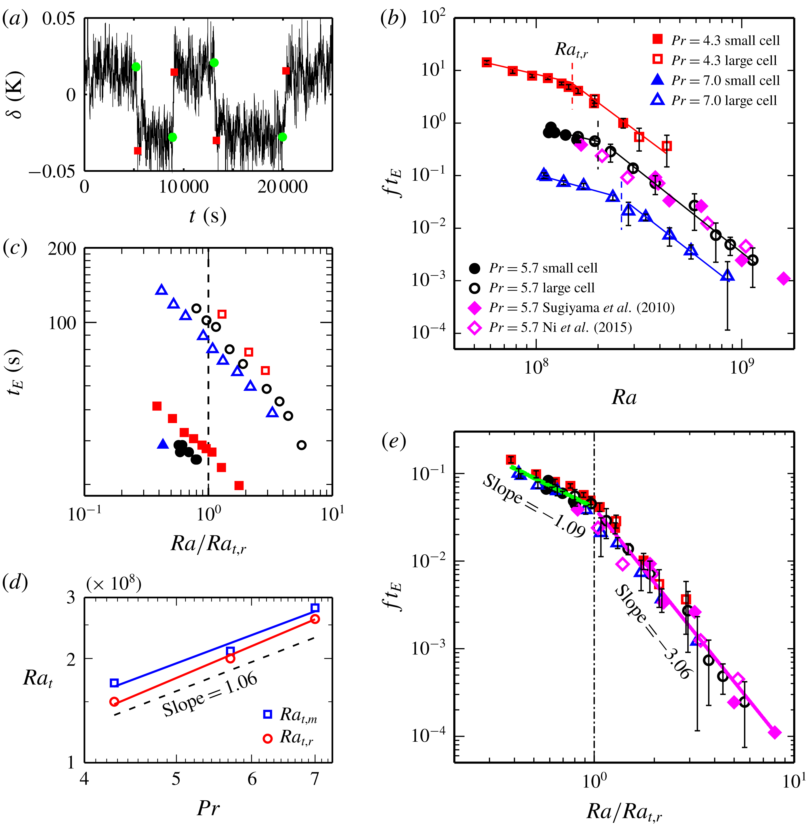
Based on the fact that in the bottom plate the temperature is higher where the hot plumes are emitted than where the cold plumes arrive, the reversal events were detected by the temperature contrast between the thermistors embedded on the left and right sides of the plates, $\unicode[STIX]{x1D6FF}=T_{left}-T_{right}$ (Sugiyama et al. Reference Sugiyama, Ni, Stevens, Chan, Zhou, Xi, Sun, Grossmann, Xia and Lohse2010; Huang & Xia Reference Huang and Xia2016). Figure 1(a) is a typical time segment of temperature contrast $\unicode[STIX]{x1D6FF}$ measured from the bottom plate, which shows how reversals were identified. The criteria we used to identify the reversal event from the time trace of $\unicode[STIX]{x1D6FF}$ are adopted from Huang & Xia (Reference Huang and Xia2016). Here we only give a brief introduction of the three criteria. The first criterion is that the two circulation states of the LSC (clockwise direction and counter-clockwise direction) should be clearly distinguished from each other. This implies that the probability density function (PDF) of $\unicode[STIX]{x1D6FF}$ (see figure 2(d) of Huang & Xia (Reference Huang and Xia2016)) should have two peaks (two most probable values), with each peak corresponding to one circulation state, and the distance between the two peaks in the PDF should be larger than the root mean squared value of $\unicode[STIX]{x1D6FF}$ , so that the two peaks can be clearly distinguished. The second criterion is that when the flow changes from one state to the other, $\unicode[STIX]{x1D6FF}$ should first cross over the peak corresponding to the current circulation state (i.e. the value of $\unicode[STIX]{x1D6FF}$ should be greater (lesser) than the larger (smaller) peak value of $\unicode[STIX]{x1D6FF}$ in the PDF). The third criterion is that the flow should stay at the new circulation state for more than one turnover time of the LSC. With these criteria, we are ready to identify the flow reversals.

Figure 1.

(a) A time segment of the temperature contrast $\unicode[STIX]{x1D6FF}$ for $Ra=3.55\times 10^{8}$ and $Pr=5.7$ . The green solid circles and red solid squares represent the starts and ends of flow reversal events. (b) Flow reversal rate $f$ (normalized by $1/t_{E}$ ) as a function of $Ra$ for different $Pr$ , where $t_{E}$ is the turnover time of the LSC. For clarity, the data for $Pr=5.7$ and 4.3 are shifted up by a factor of 10 and 100, respectively. The solid lines are the power-law fits to the data and the vertical dashed lines indicate the transitional Rayleigh number $Ra_{t,r}$ . (c) Measured $t_{E}$ as functions of $Ra$ for three different $Pr$ ; $Ra$ is normalized by $Ra_{t,r}$ . (d) The transitional $Ra$ number $Ra_{t}$ ( $Ra_{t,r}$ and $Ra_{t,m}$ ) as a function of $Pr$ . The solid lines are power-law fits to the data. The dashed line is from our model prediction (see text for details). (e) The same data sets as in (b), but $Ra$ is normalized by $Ra_{t,r}$ . The green and magenta solid lines are the power-law fits to the data before and after the transition, irrespective of the different $Pr$ .

3 Results and discussion

We first examine the $Ra$ dependence of the normalized reversal rate $f$ for different $Pr$ , as shown in figure 1(b). For clarity, the data for $Pr=5.7$ and 4.3 are shifted up by a factor of 10 and 100, respectively. Here, the reversal rate $f$ is defined as the averaged number of reversals per unit time and is non-dimensionalized by the turnover time of the LSC, $t_{E}$ , which is obtained by the cross-correlation of the temperature signals inside the plates (Brown, Funfschilling & Ahlers Reference Brown, Funfschilling and Ahlers2007). One can see that the reversal rate decreases with increasing $Ra$ (i.e. it is harder (or less probable) for reversals to occur at higher $Ra$ ). The measurement time for the reversal rate varies from one day for low $Ra$ , where the reversal is very frequent, to at least three days for high $Ra$ , where the reversal is not frequent. To obtain enough statistics, the longest measurement time for reversal rate lasted for 16 days. The decreasing reversal rate with $Ra$ shown in figure 1(b) is consistent with previous studies (Sugiyama et al. Reference Sugiyama, Ni, Stevens, Chan, Zhou, Xi, Sun, Grossmann, Xia and Lohse2010; Ni et al. Reference Ni, Huang and Xia2015). What is new here is that the $Ra$ dependence of reversal rate exhibits two distinct regimes separated by a transitional $Ra$ ( $Ra_{t,r}$ ): a slow decay regime and a fast decay regime, with very different scaling exponents. This transition is found to exist for all the $Pr$ explored. To make sure that the transition of $ft_{E}$ is indeed from $f$ , not from $t_{E}$ , we plot in figure 1(c) the measured $t_{E}$ as functions of $Ra$ for three different $Pr$ . It is seen from the figure that $t_{E}$ does not show any transition, thus the transition is indeed from $f$ . Please note that $t_{E}$ from the small convection cell (solid symbols) and that from the large convection cell (open symbols) differ by a numerical factor, because the characteristic time scales of the flows in these two cells are different. This is exactly the reason we used $t_{E}$ to non-dimensionalize $f$ . With this non-dimensionalization the cell size dependence of $f$ is eliminated. The reason that the transition was not found in previous experimental studies (Sugiyama et al. Reference Sugiyama, Ni, Stevens, Chan, Zhou, Xi, Sun, Grossmann, Xia and Lohse2010; Ni et al. Reference Ni, Huang and Xia2015) is that in those experiments the $Ra_{t,r}$ is very close to the lower end of their $Ra$ range, thus there are almost no data points when $Ra<Ra_{t,r}$ . To examine $Ra_{t,r}$ quantitatively, we take its value as being the intersecting point of the power-law fits to the two regimes for each $Pr$ . Figure 1(d) shows that $Ra_{t,r}$ increases with $Pr$ and their relationship, for the limited data points and $Pr$ range, may be described as $Ra_{t,r}\sim Pr^{1.12\pm 0.07}$ . Most interestingly, once the $Ra$ -dependent $ft_{E}$ values of different $Pr$ numbers are normalized by $Ra_{t,r}$ , all the data fall on top of each other, with the two distinct scaling regimes being $ft_{E}\sim Ra^{-1.09\pm 0.15}$ and $ft_{E}\sim Ra^{-3.06\pm 0.16}$ (see figure 1 e). The excellent collapse of different data sets implies that the transition observed here is universal, and $Ra_{t,r}$ should be underpinned by a general mechanism.

Figure 2.

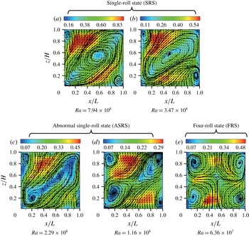
Short-time-averaged (within one LSC turnover time $t_{E}$ ) PIV velocity maps with streamlines measured at different $Ra$ for $Pr=7.0$ . The velocity is coded with both colour and vector length in units of cm s $^{-1}$ . (a–d) are measured from the large cell, (e) is measured from the small cell.

To understand the physical origin of $Ra_{t,r}$ , we first examine how the large-scale flow evolves with $Ra$ using particle image velocimetry (PIV) (Dantec Dynamics). The $Ra$ number ranges of PIV measurements for $Pr=4.3$ , 5.7 and 7.0 are $1.62\times 10^{8}$ to $1.37\times 10^{9}$ , $1.18\times 10^{8}$ to $1.12\times 10^{9}$ and $6.36\times 10^{7}$ to $7.94\times 10^{8}$ , respectively. The PIV measurements were made in the vertical midplane of the convection cells and lasted for at least two hours (corresponding to 50 to 360 $t_{E}$ ) for each $Ra$ , such that at least 7200 vector maps were acquired (sampling $\text{rate}=1$  Hz). Figure 2 shows the typical velocity fields at five different $Ra$ for $Pr=7.0$ , which is averaged over a short time period of ${\sim}t_{E}$ (from approximately 20 to 150 seconds depending on the $Ra$ and the cell size) without reversal occurring. It is seen that for large $Ra$ ( $Ra=7.94\times 10^{8}$ , figure 2 a), the flow consists of a main roll of a tilted-ellipse shape and two corner rolls diagonally opposite to each other. This flow pattern has been commonly observed in previous studies, and it is referred to as the single-roll state (SRS). When $Ra$ decreases to $3.47\times 10^{8}$ (figure 2 b), the LSC becomes slimmer, but keeps its single-roll shape. As $Ra$ further decreases to $2.29\times 10^{8}$ (figure 2 c), the flow structure becomes surprisingly different: the inner core of the main roll breaks into two smaller rolls, which nevertheless remain enclosed by the outer shell of the main roll. Such an abnormal LSC with substructures becomes more obvious when $Ra$ decreases further to $1.16\times 10^{8}$ (figure 2 d). It is clear from figure 2(d) that the main roll is severely squeezed and the two enclosed smaller rolls have grown larger and stronger. Here, although the interior of the LSC is already broken, the outer shell of the LSC keeps the interior of the LSC whole, thus the LSC can still be regarded as in the single-roll state, but with substructures inside. We name this new flow state the abnormal single-roll state (ASRS). Finally, if $Ra$ becomes even smaller ( $Ra=6.36\times 10^{7}$ , figure 2 e), the single-roll structure is replaced by a four-roll state (FRS) (i.e. the LSC is now completely broken down). As in the lower- $Ra$ regime (for example, $Ra<10^{8}$ for $Pr=7.0$ ), FRS dominates the flow and LSC no longer exists, let alone the reversal of the LSC. That is the reason we do not have the reversal rate data for the low- $Ra$ range in figure 1(b) (for example, $Ra<10^{8}$ for $Pr=7.0$ ).

Thus, we have identified a transition in the LSC structure from direct velocity measurement. Comparing with the transition observed in $ft_{E}$ , we find the transition from SRS to ASRS occurs roughly at $Ra_{t,r}$ . This suggests that in the SRS the reversal rate follows the fast decay behaviour, while in the ASRS the slow decrease of reversal rate comes into play. This correspondence between the transitions of the LSC structure and the reversal rate is found to be true for the other two $Pr$ cases. To understand why the difference in the LSC structure can lead to such a change in the $Ra$ dependence of reversal rate, we recall that reversal in the present rectangular geometry is a process in which the two diagonally opposite corner rolls break up the LSC and then connect to form a new large roll (Sugiyama et al. Reference Sugiyama, Ni, Stevens, Chan, Zhou, Xi, Sun, Grossmann, Xia and Lohse2010; Chandra & Verma Reference Chandra and Verma2013). In other words, the corner rolls have to overcome the ‘energy barrier’ (Sreenivasan et al. Reference Sreenivasan, Bershadskii and Niemela2002) due to the LSC structure, including both the inner core and outer shell. This is the case for the SRS. However, for the ASRS, as the inner core of the LSC has been broken, the ‘energy barrier’ now mainly comes from the outer shell of the LSC, and thus should be much lower than that of the SRS case. As the inner core and outer shell exhibit distinct strengths and dynamic scalings with $Ra$ (Xia, Sun & Zhou Reference Xia, Sun and Zhou2003), it is natural to expect that the ‘energy barriers’ for the occurrence of reversals in the SRS and ASRS are very different; hence resulting in the transition of the reversal rate. While it is unclear at this stage why the $Ra$ -dependent exponents of reversal rate should be $-3.06$ and $-1.09$ for the SRS and ASRS, respectively, the present finding sends an insightful message that, although it is the corner rolls that cause reversals in the present geometry, the level of difficulty (or the probability) for reversals to occur depends mainly on the ‘energy barrier’ dictated by the main roll.

Figure 3.

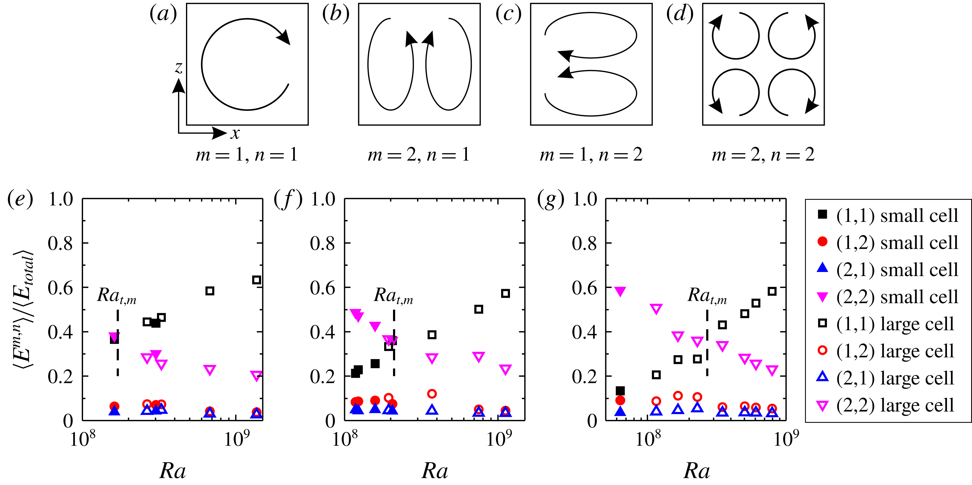
(a–d) Cartoon patterns of the first four Fourier modes. (e–g) Time-averaged energy contained in each flow mode as a function of $Ra$ for $Pr=4.3$ , 5.7 and 7.0, respectively. The dashed line shows the value of $Ra$ where the cross-over between $A^{1,1}$ and $A^{2,2}$ occurs (i.e. $Ra_{t,m}$ ).

To verify the above qualitative picture, we examine the flow energy using Fourier mode decomposition (Chandra & Verma Reference Chandra and Verma2013; Wagner & Shishkina Reference Wagner and Shishkina2013; Chong et al. Reference Chong, Wagner, Kaczorowski, Shishkina and Xia2018). Briefly, each instantaneous velocity field $\left(u_{x},u_{z}\right)$ is projected onto the Fourier modes, given as

(3.1) $$\begin{eqnarray}\displaystyle & \displaystyle u_{x}^{m,n}=2\sin (m\unicode[STIX]{x03C0}x)\cos (n\unicode[STIX]{x03C0}z), & \displaystyle\end{eqnarray}$$

(3.2) $$\begin{eqnarray}\displaystyle & \displaystyle u_{z}^{m,n}=-2\cos (m\unicode[STIX]{x03C0}x)\sin (n\unicode[STIX]{x03C0}z), & \displaystyle\end{eqnarray}$$

where $m$ and $n=1$ , 2, 3 (i.e. the first nine modes) are considered. Then the instantaneous amplitude of each mode $A^{m,n}(t)$ is obtained by making componentwise projections of each velocity field on the Fourier modes: $A^{m,n}(t)=\langle u_{x}(t)u_{x}^{m,n}\rangle _{x,z}+\langle u_{z}(t)u_{z}^{m,n}\rangle _{x,z}$ . In turn, the energy of each flow mode can be evaluated as $E^{m,n}(t)=[A^{m,n}(t)]^{2}$ (Xi et al. Reference Xi, Zhang, Hao and Xia2016). As the first four flow modes (i.e. (1,1), (2,1), (1,2) and (2,2); see their cartoon patterns in figure 3(a–d)) contribute most of the energy in the flow, we first check how their mean energy $\langle E^{m,n}(t)\rangle$ (normalized by the total flow energy $\langle E_{total}\rangle$ ) depends on $Ra$ . Figure 3(e–g) show the mean energy contained in each of the first four Fourier modes as a function of $Ra$ . It is seen from the figure that both the (2,1) and (1,2) modes are negligibly weak over the whole $Ra$ range. On the other hand, while the (1,1) and (2,2) modes dominate the flow, they behave with opposite trends and thus there exists a cross-over $Ra$ ( $Ra_{t,m}$ ) at $\simeq 1.7\times 10^{8}$ , $\simeq 2.1\times 10^{8}$ and $\simeq 2.8\times 10^{8}$ for $Pr=4.3$ , 5.7 and 7.0, respectively. To be specific, for large $Ra$ , the (1,1) mode is dominant; with decreasing $Ra$ , the (1,1) mode becomes weaker and the (2,2) mode becomes stronger. Once $Ra$ is below $Ra_{t,m}$ , the (2,2) mode overtakes the (1,1) mode to become dominant. Previously it was shown that reversal only occurs in a restricted $Ra$ range, as shown in the reversal phase diagram of Sugiyama et al. (Reference Sugiyama, Ni, Stevens, Chan, Zhou, Xi, Sun, Grossmann, Xia and Lohse2010) (see figure 4 of their paper). Now it can be readily understood with the evolution of the different flow modes. As can be seen from figure 3(e,f,g), when $Ra$ is very small the majority of the energy of the flow is in the four-roll mode. For example, for $Pr=7.0$ , when $Ra=6.36\times 10^{7}$ , $60\,\%$ of the energy is in the four-roll mode and the LSC no longer exists, let alone the reversal of LSC. This is the reason why reversal of the LSC does not occur when $Ra$ is very small. When $Ra$ becomes very large, the majority of the flow energy is in the single-roll mode; for example, $60\,\%$ of the energy is in the single-roll mode when $Ra=1\times 10^{9}$ for $Pr=7.0$ . In this high- $Ra$ range, since the single-roll mode is very strong, it is very difficult for the corner rolls to break the main roll, then lead to a reversal; that is why no (or rare) reversal is observed when $Ra$ is very large. Taking all these factors together, our results successfully explain why reversal only occurs in a restricted $Ra$ range. We define the lower bound of the restricted $Ra$ range as being the value of $Ra$ at which the (2,2) mode contains $50\%$ of the total flow energy, and the higher bound as being the $Ra$ at which the (1,1) mode contains $60\,\%$ of the total flow energy. The so-defined $Ra$ ranges agree reasonably well with the phase diagram of Sugiyama et al. (Reference Sugiyama, Ni, Stevens, Chan, Zhou, Xi, Sun, Grossmann, Xia and Lohse2010) in the $Pr$ range of our experiments. One may use different thresholds to define the $Ra$ range, but the nature of the $Ra$ range and its $Pr$ dependence do not change much.

It should be noted the non-normalized energy of the (1,1) and (2,2) modes $E^{1,1}$ and $E^{2,2}$ both increase with $Ra$ , while $E^{1,1}$ increases much faster than $E^{2,2}$ , and thus the relative weight of $E^{2,2}$ decreases. $E^{1,1}$ and $E^{2,2}$ cross each other at $Ra_{t,m}$ . This behaviour was previously observed in the numerical simulation by Chandra & Verma (Reference Chandra and Verma2013). We now show the experimental evidence. However, our results are not consistent with the experimental results of Horstmann et al. (Reference Horstmann, Schiepel and Wagner2018), who found in a cell of lateral aspect ratio $1:4$ that the amplitudes of the first two modes do not have a strong $Ra$ dependence in the $Ra$ range of our experiments; the reason for this inconsistency is not known to us. It is found that $Ra_{t,m}$ is very close to the transitional $Ra$ between ASRS and SRS; thus from now on we will not distinguish between the former and the latter. Because the (1,1) and (2,2) modes are mostly contributed by the main roll and the corner rolls, respectively, the flow-mode evolution essentially provides a quantitative description of the flow pattern evolution shown in figure 2, and thus explains the transition of the reversal rate. To confirm this, we identified the $Ra_{t,m}$ values for the three $Pr$ numbers. The obtained results plotted in figure 1(d) show that, indeed, the $Ra_{t,m}$ identified from flow-modes evolution are consistent with the $Ra_{t,r}$ determined from the reversal rate. Based on the relation: $Ra_{t}\sim Pr^{1.12}$ from figure 1(d), we predict that the $Ra_{t,m}$ for the result in Chandra & Verma (Reference Chandra and Verma2013) (where $Pr=1$ ) is approximately $2.89\times 10^{7}$ , which is very close to the cross-over $Ra$ ( ${\sim}2\times 10^{7}$ ) in figure 2 of Chandra & Verma (Reference Chandra and Verma2013).

Figure 4.

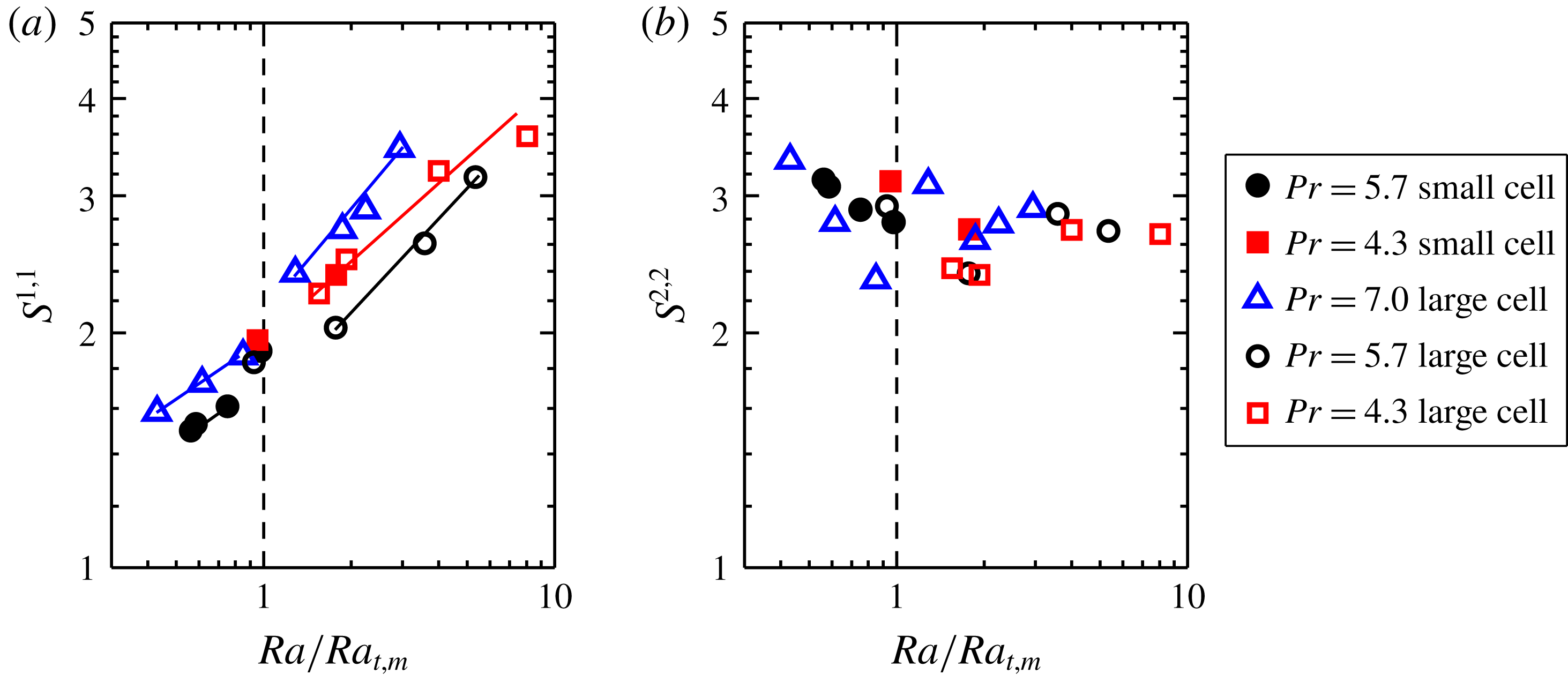
(a) The stability of the (1,1) mode $S^{1,1}=\langle A^{1,1}\rangle /\unicode[STIX]{x1D70E}_{A^{1,1}}$ and (b) the stability of the (2,2) mode $S^{2,2}=\langle A^{2,2}\rangle /\unicode[STIX]{x1D70E}_{A^{2,2}}$ as functions of the normalized $Ra$ and for three values of $Pr$ . The solid lines in (a) are the power-law fits. The data points very close to the transitional $Ra$ are not included in the fittings.

The consistency between $Ra_{t,m}$ and $Ra_{t,r}$ could not explain why the reversal rate has distinct $Ra$ dependences before and after the transition. To answer this question, we further examine the stability of the (1,1) mode, which is defined as its mean amplitude over its root mean squared value $S^{1,1}=\langle A^{1,1}\rangle /\unicode[STIX]{x1D70E}_{A^{1,1}}$ . A larger $S^{1,1}$ means a more stable main roll. Figure 4(a) shows $S^{1,1}$ as a function of $Ra$ . It is evident that there also exist two distinct regimes for $S^{1,1}$ : a slow growth regime followed by a fast growth regime. Moreover, the transitional $Ra$ of $S^{1,1}$ is almost the same as $Ra_{t,m}$ identified from flow-modes evolution and $Ra_{t,r}$ determined from the reversal rate. Figure 4(b) shows the stability of the (2,2) mode $S^{2,2}=\langle A^{2,2}\rangle /\unicode[STIX]{x1D70E}_{A^{2,2}}$ . In contrast to the (1,1) mode, $S^{2,2}$ , despite the somewhat scattered data, does not change significantly or exhibit any particular trend over the whole $Ra$ range, implying that the (2,2) mode does not directly compete with the (1,1) mode, and it is the stability of the main roll that determines the transition in the reversal rate observed here. It should be noted that here we study the stability of the (1,1) and (2,2) modes and their relationship with the reversal rate, we only used the data when the flow is in the ASRS or SRS (for example, $Ra>10^{8}$ for $Pr=7.0$ ) where the reversal of the LSC could happen. The data when the flow is in the FRS (for example, $Ra<10^{8}$ for $Pr=7.0$ ) is not used in figure 4, as in FRS the reversal of the LSC does not exist.

Based on the above analysis, we arrive at the following physical picture. For the abnormal single-roll state, the stability of the main roll is mainly determined by its outer shell, which means a lower energy barrier for breaking the LSC, and the stability of the main roll increases slowly with $Ra$ ; thus we observe a slower decay of the reversal frequency with $Ra$ . As for the normal single-roll state, both the outer shell and the inner core contribute to the stability of the main roll and its stability increases faster with increasing $Ra$ ; thus there is a steeper decay of the reversal rate. With this physical picture, we are now in a position to understand the $Pr$ dependence of $Ra_{t,r}$ ( $Ra_{t,m}$ ) shown in figure 1(d). It is well known that in the RB system the LSC is fed by thermal plumes (Xi, Lam & Xia Reference Xi, Lam and Xia2004). These plumes lose their kinetic energy via viscous dissipation when traversing the turbulent bulk. An abnormal single-roll state means that some hot (cold) plumes lose all their energy at the half-height and then fall down (turn back up) to form small rolls inside the main roll. Therefore, $Ra_{t,r}$ (i.e. the critical condition for the interior of the main roll to break up) can be quantified by the balance between the plume travel time $\unicode[STIX]{x1D70F}_{U}=H/U$ and the viscous dissipation time $\unicode[STIX]{x1D70F}_{d}=U^{2}/\unicode[STIX]{x1D700}$ . Here, $U$ is the typical velocity of the LSC and $\unicode[STIX]{x1D700}$ is the viscous dissipation rate. By making use of the definition of the Reynolds number $Re=UH/\unicode[STIX]{x1D708}$ , and the dissipation in bulk RB convection $\unicode[STIX]{x1D700}=\unicode[STIX]{x1D708}^{3}H^{-4}NuRaPr^{-2}$ (Lohse & Toschi Reference Lohse and Toschi2003), we obtain $Re^{3}\sim NuRaPr^{-2}$ . By applying our experimental results of $Re\sim$ $Ra^{0.55\pm 0.04}Pr^{-0.8\pm 0.03}$ and $Nu\sim Ra^{0.30\pm 0.02}Pr^{-0.03}$ , the balance between $\unicode[STIX]{x1D70F}_{U}$ and $\unicode[STIX]{x1D70F}_{d}$ yields $Ra_{t}\sim Pr^{1.06}$ . Here the Reynolds number in our experiments is defined as $Re=$ $2H^{2}/(\unicode[STIX]{x1D708}t_{E})$ , where $2H/t_{E}$ is the velocity scale and $2H$ is the estimate for the route length of the LSC. This result agrees remarkably well with the experimental finding $Ra_{t,r}\sim Pr^{1.12\pm 0.07}$ within uncertainty.