1 Introduction
Diapycnal turbulent mixing plays a primary role in enabling the large-scale ocean circulation (Wunsch & Ferrari Reference Wunsch and Ferrari2004). Over the past several decades, significant investment has been made in estimating the strength of diapycnal mixing on the basis of observations of ocean turbulence (see e.g. St. Laurent & Simmons Reference St. Laurent and Simmons2006; Waterhouse et al. Reference Waterhouse, Mackinnon, Nash, Alford, Kunze, Simmons, Polzin, St Laurent, Sun and Pinkel2014, for reviews). Four common assumptions concerning density stratified turbulence, made for practical purposes in conventional methods employed for the estimation of mixing from observations, are that the turbulence is (I) fully developed, (II) stationary, (III) and isotropic and that (IV) there exists a clear separation of scales between the background mean flow and the superposed isotropic turbulence. In recent years, numerical simulations have become just powerful enough to aid in quantification of inaccuracies associated with these assumptions (Ivey, Winters & Koseff Reference Ivey, Winters and Koseff2008; Pham & Sarkar Reference Pham and Sarkar2010; Mashayek, Caulfield & Peltier Reference Mashayek, Caulfield and Peltier2013; Mashayek & Peltier Reference Mashayek and Peltier2013; Salehipour & Peltier Reference Salehipour and Peltier2015; Salehipour, Peltier & Mashayek Reference Salehipour, Peltier and Mashayek2015; Salehipour, Caulfield & Peltier Reference Salehipour, Caulfield and Peltier2016a ).
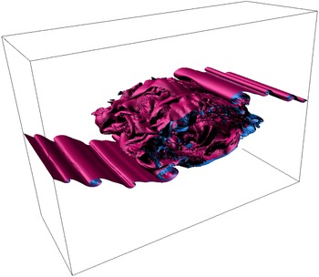
A common hypothesis is that shear-driven mixing in the ocean is at least partially induced by the breaking of internal waves excited by tides and geostrophic motions in the deep ocean or by winds at the surface (Alford & Pinkel Reference Alford and Pinkel2000; Garrett Reference Garrett2003; Nikurashin & Ferrari Reference Nikurashin and Ferrari2011). Such mixing comprises many individual breaking events each of which is non-stationary in time. It is at least plausible that some of these breaking events may be considered to be generated by shear instabilities on scales small compared to the internal waves. Such shear instability generated mixing may be characterized by a multi-stage life cycle. A preparatory period of growth of the internal wave amplitude leads to an initial period of shear instability growth, then break down through secondary instabilities triggering a transition to turbulence. This initial period is followed by an intermediate period of what might be considered to be fully developed turbulence, followed ultimately by a final decay period. Contrary to common assumptions in parameterization schemes (Mashayek & Peltier Reference Mashayek and Peltier2013), in this scenario of shear instability generated mixing the contribution of the intermediate ‘fully developed’ period does not necessarily dominate the net vertical cross-density flux of mass and tracers, even at very high flow Reynolds numbers. Furthermore, even in the most turbulent intermediate period, turbulence can be highly non-stationary and anisotropic comprising a range of scales between that of small-scale quasi-isotropic turbulence and that of the background mean flow, particularly when there is a dominant shear direction imposed by some ‘external process’, for example through the intensification of an appreciably larger-scale internal wave (Fritts et al. Reference Fritts, Bizon, Werne and Meyer2003; Ivey et al. Reference Ivey, Winters and Koseff2008; Mashayek & Peltier Reference Mashayek and Peltier2013; Mashayek et al. Reference Mashayek, Caulfield and Peltier2013). Figure 1, produced from results of a numerical simulation to be discussed in detail later, illustrates the cascade of instabilities which form upon a shear instability overturn and which eventually destroy billow coherence. As we will discuss in the paper, this anisotropic highly time-dependent turbulence transition phase of flow makes a major contribution to the net vertical mixing of mass over the entire life cycle of this type of turbulence.
Snapshot of turbulence break down and mixing due to breaking of an overturning by shear instability in a stably stratified layer (case 12 in table 1). Purple and blue represent light and heavy density iso-surfaces, respectively. The snapshot corresponds to time
 $t=80h/\unicode[STIX]{x0394}u$
, where
 $h$
is half the initial shear layer depth and
 $\unicode[STIX]{x0394}u$
is half the total velocity difference.

Recently, Mashayek & Peltier (Reference Mashayek and Peltier2013) (hereafter MP13) and Mashayek et al. (Reference Mashayek, Caulfield and Peltier2013) (hereafter MCP13) presented computation-based evidence for break down of assumptions I–III when the turbulence is triggered by a initial shear instability. In two important papers (Smyth & Moum Reference Smyth and Moum2000a ,Reference Smyth and Moum b ), Smyth and Moum effectively addressed assumptions III and IV (though they did not couch the discussion in precisely those terms). Crucially, their simulations were at significantly lower Reynolds number than is now achievable, and thus in particular the shear instabilities they simulated were not prone to the full ‘zoo’ of secondary instabilities identified in Mashayek & Peltier (Reference Mashayek and Peltier2012a ,Reference Mashayek and Peltier b ), and so their subsequent analysis of the turbulence properties is inevitably affected by the absence of physical processes present in geophysically relevant higher Reynolds number flows. In this study, we build on the work of Smyth & Moum (Reference Smyth and Moum2000a ) (hereafter SM00) to focus on assumption IV, analysing data from a more complete set of numerical simulations at substantially higher Reynolds number closer to values representative of energetic ocean mixing zones. In particular we will extend their analysis of scales of turbulence. Through this analysis, we demonstrate that assumption IV may at best hold in only a rather narrow part of the life cycle for rather special shear instabilities, implying that extending a model based fundamentally on this assumption over the whole turbulence life cycle may well introduce large uncertainty and/or inaccuracy in estimates of net turbulent mixing over the life cycle of an individual wave breaking event, if that wave breaking is generated by the onset of shear instabilities. Wave-induced turbulence in energetic oceanic regions is determined by the combination of many individual breaking events, both essentially isolated in space and time and yet dynamically coupled in some way. Therefore, there is no a priori basis upon which it can be assumed that the inaccuracies we discuss in this work will have negligible effect in the much more complex real ocean. Of course, it is always important to remember that our results are based on modelling individual wave breaking events in the highly idealized configuration that the vertical shear and density distribution induced by the intensification of the internal waves may be taken to be at least quasi-steady on the time scale of the development of shear instabilities on those distributions.
There has been an increasing recent interest in description of shear-induced density stratified turbulent mixing in terms of key physical length scales (see e.g. Mater, Schaad & Venayagamoorthy Reference Mater, Schaad and Venayagamoorthy2013; Scotti Reference Scotti2015), and we will focus herein on the critical importance of the time dependence of characteristic length scales for mixing in a stratified shear flow. Understanding the relative time dependence of length scales within the flow is of general interest, as estimates of diapycnal mixing are often constructed from instantaneous measurements of specific length scales (see Thorpe Reference Thorpe2005, for an overview).
Employing shear instability as a canonical mixing agent, our focus will be upon the lasting effect of the primary ‘overturning’ associated with the primary shear instability which leads to ‘efficient’ (in a way we define precisely in § 6) irreversible mixing. An important implication of our analyses is that mixing efficiencies may be under-estimated in regions of the ocean in which large overturns are expected since they provide a significant reservoir of energy upon which a broad inertial subrange of turbulence may draw so as to support efficient irreversible mixing. The most or ‘optimal’ efficient mixing will be shown to occur at the instant during flow evolution when the scale at which energy is injected, through overturning into the turbulence cascade at the upper bound of the inertial subrange becomes sufficiently small to avoid suppression by the ambient stratification. This core idea (as we discuss further below) is consistent with the arguments presented by Ivey & Imberger (Reference Ivey and Imberger1991), though for our flows, the associated value of the mixing efficiency in this ‘optimal’ situation is found to be higher. Of course it will remain an important issue as to whether the specific model of shear instability generated turbulence that we will employ as basis for our analyses, relying upon the classical Kelvin–Helmholtz instability (KHI), may be considered sufficiently representative of spatio-temporally intermittent, relatively large-scale wave breaking processes in general to enable our results to stand without caveat. For example, one key issue is the role of ambient, larger-scale background stratification in the development and break down of shear instabilities. There does exist evidence, however, in support of the relevance of KHI-based analysis for the understanding of stratified turbulence in general (Smyth, Moum & Caldwell Reference Smyth, Moum and Caldwell2001; Bouffard & Boegman Reference Bouffard and Boegman2013; Scotti Reference Scotti2015). We will provide some of the evidence of the generality of the utility of this model of stratified turbulent processes by comparing results from direct numerical simulations with observations.
This paper is organized as follows. In § 2 we briefly describe the suite of turbulence simulations upon which our analyses will be based. Section 3 will provide definitions of the important length scales that may be employed to characterize shear-driven stratified mixing events. Section 4 presents a detailed discussion of the time dependence of the evolution of these scales, focusing especially on what may be considered their generic behaviour in stratified shear-driven mixing at sufficiently high Reynolds number. In § 5 we discuss the importance of the relative evolution of the Ozmidov and Thorpe length scales for quantification of the age of turbulence. In § 6 we briefly discuss the implications of our results and in particular discuss in § 5 the quantitative representation of mixing in geophysically relevant circumstances. Conclusions are offered in the final § 7.
2 Primary shear instability
In this section we discuss the numerical datasets that will be employed to study turbulence transition of primary shear instabilities as well as the bulk dimensionless parameters which characterize them.
2.1 Numerical simulations
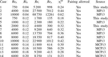
We employ a suite of high resolution direct numerical simulations (DNS) of the turbulence life cycle of finite-amplitude Kelvin–Helmholtz instability (KHI) billows in stratified shear layers, a common mechanism leading to turbulence transition in the ocean (Smyth & Moum Reference Smyth and Moum2012; Mashayek Reference Mashayek2013). The data to be employed are summarized in table 1 and consist of the same set of numerical simulations as were previously analysed in MP13 and MCP13 for other purposes, augmented by three new simulations, as noted in the table. Each of these simulations describes the three-dimensional temporal evolution of a horizontally periodic stably stratified shear layer with the initial background velocity profile
 $\bar{u}(z)$
and Boussinesq density profile
 $\bar{\unicode[STIX]{x1D70C}}(z)$
defined as
 $$\begin{eqnarray}\bar{u}(z)=\unicode[STIX]{x0394}u\tanh \left(\frac{z}{h}\right)\!;\quad \bar{\unicode[STIX]{x1D70C}}(z)=\unicode[STIX]{x1D70C}_{a}-\unicode[STIX]{x0394}\unicode[STIX]{x1D70C}\tanh \left(\frac{z}{h}\right),\end{eqnarray}$$
where
 $\unicode[STIX]{x0394}u$
and
 $\unicode[STIX]{x0394}\unicode[STIX]{x1D70C}$
are half the velocity and density variation,
 $h$
is half the shear layer thickness and
 $\unicode[STIX]{x1D70C}_{a}\gg \unicode[STIX]{x0394}\unicode[STIX]{x1D70C}$
is the reference density. As reviewed in MP13, this configuration has come to be seen as a the standard model problem for the study of mixing induced by large-scale overturning shear instabilities. As noted in the introduction, there is an underlying assumption that this background flow distribution may be taken to be steady, and so if it is induced by the intensification of an even larger-scale internal wave, the evolution of that wave occurs on time scales which are long compared to the time scales of the evolution of the primary shear instability of this flow distribution.
Parameter values for the numerical simulations analysed in this paper.
 $Pr=1$
for all cases. The initial Reynolds number
 $Re_{0}$
, the initial minimum Richardson number at
 $z=0$
 $Ri_{0}$
, the effective Reynolds number
 $Re_{t}$
at the start of the fully developed turbulent period
 $t_{3D}^{S}$
and the cumulative turbulent mixing efficiency
 $\unicode[STIX]{x1D702}_{c}^{3D}$
are all defined in the text.

2.2 Governing dimensionless parameters
Three non-dimensional numbers characterize the flow for each case, namely an appropriate Reynolds number
 $Re$
, quantifying the ratio of inertial to viscous forces, an appropriate Richardson number
 $Ri$
, quantifying the ratio of buoyancy to inertial forces and the Prandtl number
 $Pr=\unicode[STIX]{x1D708}/\unicode[STIX]{x1D705}_{m}$
, the ratio of molecular kinematic viscosity to molecular thermal diffusivity. The initial Reynolds number
 $Re_{0}=\unicode[STIX]{x0394}u~h/\unicode[STIX]{x1D708}$
for each of the simulations of turbulent collapse to be analysed is listed in table 1, and is defined based on a length scale that is half the shear layer thickness and a velocity scale that is half the velocity difference across the initial density inversion upon which the shear is imposed prior to its evolution through primary instability into the classical Kelvin–Helmholtz billow form. Indeed, since we are primarily interested in the turbulent phase of flow evolution, the nonlinear Kelvin–Helmholtz billow itself being an essentially laminar structure, a more relevant definition of the Reynolds number might be one based upon a length scale determined by the half-shear layer thickness at the onset of turbulence (to be defined in (3.2)), which is larger than the initial layer’s half-thickness. This modified Reynolds number is denoted by
 $Re_{t}>Re_{0}$
in the table and might usefully be viewed as the relevant parameter for comparison with shear instabilities observed in nature.
Turbulent mixing events associated with the evolution of a Kelvin–Helmholtz billows are strongly time dependent and transient. Therefore, it is appropriate to define a criterion to identify the time of onset of turbulence which may be considered to be ‘fully developed’. Following Caulfield & Peltier (Reference Caulfield and Peltier2000) and MP13, we monitor the inherently three-dimensional turbulent kinetic energy at scales smaller than the Ozmidov scale (representing the size of the largest eddies not suppressed by stratification; to be defined in the next section). Generically, this scale-selected turbulent kinetic energy reaches a maximum magnitude (with respect to time) following a rapid growth during turbulence transition associated with the break down of the primary Kelvin–Helmholtz billow. We identify the onset of what we refer to as fully developed turbulence with this time of maximum magnitude, which time was named
 $t_{3D}^{S}$
(or
 $t_{3D}$
when context allowed) in Mashayek et al. (Reference Mashayek, Caulfield and Peltier2013), and
 $Re_{t}$
is also evaluated at this time.
It is important to remember that our convention for the definition of
 $Re_{0}$
is different from that used by SM00, which used the total shear layer depth and the total velocity difference. Using our convention, their simulations had
 $340<Re_{0}<1250$
, with the majority of the simulations being conducted at
 $Re_{0}\simeq 500$
. As we demonstrate further below, the absence of the full ‘zoo’ of instabilities discussed in Mashayek & Peltier (Reference Mashayek and Peltier2012a
) and Mashayek & Peltier (Reference Mashayek and Peltier2012b
) means the properties of flows with such Reynolds numbers are qualitatively different from flows with
 $Re_{0}\gtrsim 4000$
in this ‘fully developed’ turbulence stage of flow evolution, and so it is of value to revisit and extend their analyses at such larger
 $Re_{0}$
.
The (minimum) bulk Richardson number,
 $Ri_{0}=g\unicode[STIX]{x0394}\unicode[STIX]{x1D70C}h/(\unicode[STIX]{x1D70C}_{a}(\unicode[STIX]{x0394}u)^{2})$
, which applies initially at the midpoint of the shear layer, is also listed in the table. To keep the problem tractable, for practical reasons we avoid varying the Prandtl number and set
 $Pr=\unicode[STIX]{x1D708}/\unicode[STIX]{x1D705}_{m}=1$
. It is important, however, to appreciate that there is recent evidence that the small-scale characteristics of turbulent mixing are affected by larger, more physically relevant values of
 $Pr$
(Klaassen & Peltier (Reference Klaassen and Peltier1985a
), SM00, Mashayek & Peltier (Reference Mashayek and Peltier2011), Bouffard & Boegman (Reference Bouffard and Boegman2013), Salehipour & Peltier (Reference Salehipour and Peltier2015), Salehipour et al. (Reference Salehipour, Peltier and Mashayek2015)) even at relatively high values of the Reynolds number. A further important non-dimensional parameter, insofar as the characteristics of stratified turbulent mixing are concerned, is the so-called buoyancy Reynolds number
 $Re_{b}$
:
 $$\begin{eqnarray}Re_{b}={\mathcal{E}}/(\unicode[STIX]{x1D708}N^{2}),\end{eqnarray}$$
where here we define this parameter in terms of an appropriately externally determined buoyancy frequency ‘
 $N$
’ and the (total) kinetic energy dissipation rate
 ${\mathcal{E}}$
, defined as
 $$\begin{eqnarray}{\mathcal{E}}=\frac{\unicode[STIX]{x1D708}}{2V}\int \left(\frac{\unicode[STIX]{x2202}u_{i}}{\unicode[STIX]{x2202}x_{j}}+\frac{\unicode[STIX]{x2202}u_{j}}{\unicode[STIX]{x2202}x_{i}}\right)^{2}\,\text{d}V,\end{eqnarray}$$
where
 $V$
is the volume of the part of the domain that encompasses the mixing layer (to be defined in the next section), and the Einstein summation convention has been employed. Consistent with the scaling arguments originally presented by Gibson (Reference Gibson1980) in support of his concept of ‘fossil turbulence’, energetic stratified turbulence can be maintained in a form not substantially affected by viscosity for
 $Re_{b}\sim O(10^{2})$
or higher with viscous suppression occurring once
 $Re_{b}$
falls below
 ${\sim}O(10)$
(Ivey & Imberger (Reference Ivey and Imberger1991), SM00, Thorpe (Reference Thorpe2005), Ivey et al. (Reference Ivey, Winters and Koseff2008)). While
 $O(10^{2})<Re_{b}<O(10^{3})$
is estimated to be relevant to mixing events in the thermocline and upper (pelagic) ocean, values of
 $Re_{b}\sim O(10^{3})$
and larger have been reported in the energetic abyssal oceans where mixing plays a key role in maintaining the ocean meridional overturning circulation (Gargett, Osborn & Nasmyth Reference Gargett, Osborn and Nasmyth1984; Itsweire et al.
Reference Itsweire, Koseff, Briggs and Ferziger1993; Smyth & Moum Reference Smyth and Moum2001; Thorpe Reference Thorpe2005; Mashayek et al.
Reference Mashayek, Salehipour, Bouffard, Caulfield, Ferrari, Nikurashin, Peltier and Smyth2017).
Despite many attempts to characterize stratified turbulence in terms of
 $Re_{b}$
alone, it is well known that on the basis of both dimensional argument and physical understanding it is not sufficient (Mashayek Reference Mashayek2013; Mater & Venayagamoorthy Reference Mater and Venayagamoorthy2014; Salehipour et al.
Reference Salehipour, Peltier, Whalen and MacKinnon2016b
). A key issue concerning the use of
 $Re_{b}$
alone to classify and parametrize turbulence properties in a stratified flow is the time dependence of the dissipation rate
 ${\mathcal{E}}$
(and indeed the spatial dependence of dissipation when not spatially averaged), making it problematic to identify a particular value of
 $Re_{b}$
with a specific mixing event. Indeed, for shear-driven turbulence, the dissipation rate
 ${\mathcal{E}}$
varies strongly with time, and does not actually exhibit any period when it is not varying strongly. Therefore, it is appropriate to think of a particular mixing event as sampling a range of
 $Re_{b}$
, typically growing to a maximum value rapidly as the flow undergoes the transition to turbulence, before decaying with time as the flow relaminarizes.
Finally, the range of
 $Ri_{0}$
considered in this study is
 $0.04<Ri_{0}<0.2$
. For the particular velocity and density profiles defined in (2.1),
 $Ri_{0}$
is the minimum initial value of the (local) gradient Richardson number
 $Ri_{g}(z,t)$
defined as
 $$\begin{eqnarray}Ri_{g}(z,t)=\frac{-\displaystyle \frac{g}{\unicode[STIX]{x1D70C}_{a}}\frac{\unicode[STIX]{x2202}\langle \unicode[STIX]{x1D70C}\rangle }{\unicode[STIX]{x2202}z}}{\displaystyle \left(\frac{\unicode[STIX]{x2202}\langle u\rangle }{\unicode[STIX]{x2202}z}\right)^{2}},\end{eqnarray}$$
where angle brackets denote horizontal averaging. The bound
 $Ri_{0}=0.2$
is chosen to be below the classical value of
 $1/4$
for the global minimum value of
 $Ri_{g}$
associated with linear stability of stratified shear flows, according to the Miles–Howard criterion (Howard Reference Howard1961; Miles Reference Miles1961).
 $Ri_{0}$
represents the minimum Richardson number in the pre-turbulent shear layer and so cannot be directly compared to observation-based local estimates of
 $Ri_{0}$
, since such observation-based estimates are inevitably bulk estimates, due to the lack of resolution in the measurement of background shear. An effective bulk measure of the Richardson number
 $Ri$
based on velocity and density jumps across the entire vertical extent of the mixing region in our simulations is typically
 ${\sim}O(1)$
throughout the turbulent phase of flow evolution.
Cases in table 1 are divided into two categories with respect to the possibility of an upscale cascade through pairing instability. The simulations previously reported in MP13 extended over two wavelengths of the primary shear instability in the streamwise direction, thus allowing for pairing to occur. However, it was shown in MP13 (for
 $Pr=1$
) and Salehipour et al. (Reference Salehipour, Peltier and Mashayek2015) (for
 $Pr>1$
) that the pairing instability is suppressed as the Reynolds number increases, and that for
 $Pr=1$
, it becomes significantly diminished for
 $Re_{0}\geqslant 6000$
. Thus, the simulations in MCP13 (which were all for
 $Re_{0}=6000$
) imposed streamwise periodicity over only one wavelength of the primary instability. However, as we discuss below in more detail, the degree to which pairing is diminished at high
 $Re$
influences the properties of turbulence sufficiently to bring previously suggested parameterizations of turbulence into question. Therefore, we have included both types of simulations here, clearly marking those simulations for which pairing is allowed and recognizing that if these simulations were to be repeated at even higher relevant Reynolds number the residual influence of an upscale component of the turbulent cascade could be further mitigated, if not completely eliminated.
It is important to note that in the limit of extremely small Richardson number corresponding to effectively unstratified shear layers, the transition to turbulence may be dominated by vortices which grow on the braid of KHI billows rather than in the ‘eyelids’. Such braid-centred vortices have a much longer spanwise length scale than the core-centred convective or shear instabilities (Klaassen & Peltier Reference Klaassen and Peltier1985b ; Caulfield & Peltier Reference Caulfield and Peltier1994; Smyth & Peltier Reference Smyth and Peltier1994; Potylitsin & Peltier Reference Potylitsin and Peltier1998, Reference Potylitsin and Peltier1999; Caulfield & Peltier Reference Caulfield and Peltier2000). The spanwise extent of the computational domains were selected according to their corresponding Richardson number in such a way as to resolve the expected developing secondary perturbations.
3 Definition of length scales of turbulence
In this section we introduce various length scales which we invoke to characterize certain aspects of shear-driven stratified mixing events. As discussed in SM00, a natural way to compare length scales for shear flows with different initial minimum Richardson numbers is to non-dimensionalize with the (constant for a particular simulation) length scale
 $L_{sc}$
defined as
 $$\begin{eqnarray}L_{sc}=\unicode[STIX]{x1D70C}_{a}\unicode[STIX]{x0394}u^{2}/(4g\unicode[STIX]{x0394}\unicode[STIX]{x1D70C})=h/(4Ri_{0}),\end{eqnarray}$$
i.e. the notional length scale expressed in terms of the initial velocity difference and density difference which amounts to an initial (bulk) Richardson number with the Miles–Howard marginal value of
 $1/4$
.
We consider four dynamically determined and, crucially, inherently time-dependent characteristic length scales, namely the Kolmogorov (
 $L_{K}$
), Ozmidov (
 $L_{O}$
), Corrsin (
 $L_{C}$
) and Thorpe (
 $L_{T}$
) scales. All of these scales typically vary significantly during the three distinct periods of the turbulence life cycle discussed in the introduction: an initial or early period of transition to turbulence in which energy is transferred from the background kinetic energy into turbulent kinetic energy (TKE) due to the ‘break down’ of the organized flow; an intermediate period of sustained energetic stratified turbulence; and a final or late period during which this turbulence decays and the flow relaminarizes. We note that while
 $L_{K}$
,
 $L_{O}$
and
 $L_{C}$
are most relevant during the fully turbulent period of the flow, their formal consideration in earlier periods is helpful for the purposes of the discussions to follow.
To define these characteristic scales in an internally consistent way, it is necessary to obtain an estimate of evolution of the thickness of the initial shear and density layers upon which turbulence grows. Following SM00, we define two integral scales
 $I_{\unicode[STIX]{x1D70C}}$
and
 $I_{u}$
which track the evolution of both thicknesses during the three periods of the shear layer’s turbulent evolution:
 $$\begin{eqnarray}I_{\unicode[STIX]{x1D70C}}(t)=\int _{-L_{z}/2}^{L_{z}/2}\left[1-\left(2\frac{\langle \unicode[STIX]{x1D70C}\rangle }{\unicode[STIX]{x0394}\unicode[STIX]{x1D70C}}\right)^{2}\right]\,\text{d}z,\quad I_{u}(t)=\int _{-L_{z}/2}^{L_{z}/2}\left[1-\left(2\frac{\langle u\rangle }{\unicode[STIX]{x0394}u}\right)^{2}\right]\,\text{d}z.\end{eqnarray}$$
where angle brackets denote horizontal averaging. Both scales are defined to have the same thickness as the initial density and shear layers at the onset of the flow evolution, and will vary with time as a consequence of turbulent mixing. Since in our study the Prandtl number is 1, the ratio of these two scales is close to 1. In all definitions and analysis to be provided from this point on, spatial and volume averages are limited in the vertical to the mixing layer as defined by the above-defined time-dependent length scale
 $I_{u}(t)$
, i.e. over the interval
 $[-I_{u}/2,I_{u}/2]$
. In particular
 $Re_{t}$
in table 1 is defined using
 $I_{u}/2$
at the time when the inherently three-dimensional turbulent kinetic energy reaches its maximum value (i.e.
 $t_{3D}^{S}$
as discussed in more detail in Mashayek et al. (Reference Mashayek, Caulfield and Peltier2013)).
Using these integral scales, the instantaneous representations of background velocity shear, background buoyancy frequency and Richardson number become:
 $$\begin{eqnarray}S_{b}(t)=\frac{\unicode[STIX]{x0394}u}{I_{u}(t)},\qquad N_{b}(t)=\sqrt{\frac{g\unicode[STIX]{x0394}\unicode[STIX]{x1D70C}}{I_{\unicode[STIX]{x1D70C}}(t)}},\qquad Ri(t)=\frac{g\unicode[STIX]{x0394}\unicode[STIX]{x1D70C}/I_{\unicode[STIX]{x1D70C}}(t)}{(\unicode[STIX]{x0394}u/I_{u}(t))^{2}}=\frac{N_{b}^{2}}{S_{b}^{2}}.\end{eqnarray}$$
3.1 Thorpe scale
 $L_{T}$

The first of the four scales we discuss is the so-called ‘Thorpe scale’
 $L_{T}$
, which is a measure of net vertical parcel displacements associated with turbulent mixing. The Thorpe scale calculated from the three-dimensional numerical simulations (
 $L_{T}^{3D}$
) is determined by a sorting of the density field
 $\unicode[STIX]{x1D70C}(x,y,z,t)$
into a temporally evolving statically stable staircase of fluid parcels.
 $L_{3D}^{T}$
is then the root mean square of the vertical displacement of the particles from their actual position to the vertical position in the sorted density field. This approach follows previous studies (Winters et al.
Reference Winters, Lombard, Riley and D’Asaro1995; Caulfield & Peltier Reference Caulfield and Peltier2000). During the sorting process, the horizontal area of each fluid parcel in the mesh in terms of which the numerical simulation is described is set to that of the full domain, and its vertical thickness is adjusted so as to conserve mass. This method leads to a statically stable vertical distribution of density within the domain with the same volume (and hence mass due to the Boussinesq approximation) as the unsorted domain, but one which possesses the minimum potential energy that any adiabatic re-ordering of the discrete fluid particles in the domain could achieve at a given time during flow evolution. The root mean square of the vertical displacement that each fluid parcel experiences in this sorting procedure is by definition the three-dimensional Thorpe scale
 $L_{T}^{3D}$
. As discussed in SM00, this estimate will differ from the Thorpe scale calculated by sorting entire individual water columns, but typically that difference is found to be relatively small. More specifically, the column-wise estimate is a measure of overturnings in the flow, whereas the three-dimensional Thorpe scale is a more general representation of density displacements and is meaningful even in the absence of overturnings or when recognizably large-scale overturnings have collapsed into fine-scale turbulence. Hereafter we will choose
 $L_{T}^{3D}$
to be the appropriate time-dependent characteristic measure of overturning and will simply refer to it as
 $L_{T}$
. This is a different convention from that employed in SM00, who used
 $L_{T}$
to refer to the column-wise estimate, which must be distinguished from our full three-dimensional estimate
 $L_{T}^{3D}$
. In appendix B we discuss differences between the two and their implications for the relevance of our work to oceanographic estimates of the Thorpe scale based on column sorting.
In so far as evolution of
 $L_{T}$
in shear instabilities of KHI type is concerned,
 $L_{T}$
is expected to grow during the initial growth of the primary billows (either precursory to or concurrent with turbulence transition) and it is expected to decrease as the flow mixes thoroughly and relaminarizes. As will be discussed in what follows, the evolution of
 $L_{T}$
also depends on whether vortex pairing occurs or not. Thus, our simulations differ from those in SM00 since their simulations were initiated with an eigenmode of pairing instability. In the subset of our simulations in which the domain is sufficiently large to house vortex pairing, pairing occurs at low Reynolds number but its onset is a function of Richardson number and pairing also gets increasingly suppressed at higher Reynolds numbers. These subtle differences between the various cases discussed herein and in SM00 (independently of the wide differences in
 $Re_{0}$
) have implications for
 $L_{T}$
evolution and the relevance of
 $L_{T}/L_{O}$
as a proxy for turbulence age. We return to this in § 5.
3.2 Ozmidov length
$L_{O}$
, Corrsin length
$L_{C}$
and Kolmogorov length
$L_{K}$


The Thorpe scale
 $L_{T}$
is a purely geometrical construct, and is defined in terms of properties of the evolving density field alone, with no explicit dependence on the flow velocity field, with the connection being entirely implicit due to the evolving flow dynamics. To characterize turbulence, it is helpful to resort to length scales constructed using both intrinsic properties of turbulence such as the spatially averaged total kinetic energy dissipation rate
 ${\mathcal{E}}$
and bulk external properties such as the background density gradient and velocity shear. Ozmidov and Corrsin scales are defined in terms of such quantities. The (total) dissipation rate has dimensions
 $L^{2}T^{-3}$
, and so we define
 $L_{O}$
and
 $L_{T}$
as the two natural length scales relating the dissipation rate to the background buoyancy frequency
 $N_{b}(t)$
and the background shear
 $S_{b}(t)$
given in (3.3) through
 $$\begin{eqnarray}L_{O}(t)=\left(\frac{{\mathcal{E}}}{N_{b}^{3}}\right)^{1/2};\quad L_{C}(t)=\left(\frac{{\mathcal{E}}}{S_{b}^{3}}\right)^{1/2}\rightarrow Ri(t)=\left(\frac{L_{C}}{L_{O}}\right)^{2/3}.\end{eqnarray}$$
Physically, for vertical scales larger than both Ozmidov and Corrsin scales, turbulence with sufficiently elevated values of the dissipation rate noticeably ‘feels’ the influence of stratification and shear.
As discussed in SM00, the temporal evolution of
 $L_{C}$
and
 $L_{O}$
are broadly similar, although in general
 $L_{C}<L_{O}$
, unsurprisingly due to the relationship to
 $Ri(t)$
as defined in (3.4). In a shear layer of the kind considered here, both
 $N_{b}$
and
 $S_{b}$
decrease with time, due to the thickening of the mixing layer captured by the increases in the integral length scales
 $I_{\unicode[STIX]{x1D70C}}$
and
 $I_{u}$
respectively. Therefore, the time evolution of both
 $L_{O}$
and
 $L_{C}$
is dominated by the time dependence of the (total) dissipation rate
 ${\mathcal{E}}$
, as defined in (3.4) with both reaching their peak values during the most energetic intermediate period of turbulence in which the flow is replete with secondary and higher-order instabilities. Similarly to
 $L_{T}$
, we also expect
 $L_{O}$
(and
 $L_{C}$
) to decay as the turbulence decays, as
 ${\mathcal{E}}$
markedly decreases from its peak value.
The total dissipation rate may also be used to define a further natural length scale, namely the Kolmogorov dissipation scale
 $L_{K}$
, where
 $$\begin{eqnarray}L_{K}=\left(\frac{\unicode[STIX]{x1D708}^{3}}{{\mathcal{E}}}\right)^{1/4},\end{eqnarray}$$
and represents the scale below which the smallest eddies in the momentum field are viscously dissipated. Since in our cases
 $Pr=1$
, this is also the scale at which diffusion completely homogenizes the density field (i.e.
 $L_{K}=L_{B}=(\unicode[STIX]{x1D708}\unicode[STIX]{x1D705}_{m}^{2}/{\mathcal{E}})^{1/4}$
where the latter is the Batchelor scale). Unlike
 $L_{O}$
and
 $L_{C}$
,
 $L_{K}$
reaches its minimum value during the intermediate period when the turbulence is most energetic and hence the dissipation rate is largest. Before the flow is turbulent, or during the late turbulent decay period of the flow,
 $L_{K}$
tends to an asymptotic value set by the small finite rate of dissipation of kinetic energy associated with the laminar shear layer, since here we choose to define
 $L_{K}$
using the total dissipation rate
 ${\mathcal{E}}$
, which does not tend to zero when the flow is laminar. Similarly,
 $L_{O}$
and
 $L_{C}$
are also defined using
 ${\mathcal{E}}$
, and so these length scales are still well defined during the stage of flow evolution when the transition to turbulence is occurring.
3.3 Relative magnitudes of the scales
Consistently with the results of SM00 for flows with substantially smaller
 $Re_{0}$
, early in the flow evolution,
 $L_{T}$
can be substantially larger than
 $L_{O}$
, even when
 $L_{O}$
is defined using the total dissipation rate. We investigate this scale separation in the next section. The turbulent dynamics at this early stage is highly anisotropic due to the influence of shear and stratification on scales above the Ozmidov scale, and the properties of the turbulence can be changing rapidly. The scales between
 $L_{O}$
and
 $L_{C}$
are still anisotropic, but largely influenced by shear alone, while the scales between
 $L_{C}$
and
 $L_{K}$
may be considered to exhibit nearly isotropic three-dimensional turbulence, provided of course that there is sufficient scale separation between
 $L_{C}$
and
 $L_{K}$
to allow for an inertial cascade. Indeed, since we expect
 $L_{C}\lesssim L_{O}$
, this requirement for sufficient scale separation to allow for an inertial cascade of isotropic turbulence is typically unaffected by the background stratification.
 $L_{T}$
,
 $L_{O}$
,
 $L_{C}$
and
 $L_{K}$
are all strongly dependent on
 $Re_{0}$
and
 $Ri_{0}$
, as well as typically strongly time dependent. In § 6 we will show that the extent to which these various subranges vary, and indeed even exist in any meaningful sense, has important implications for the irreversible mixing properties of the flow.
It is important to note that while
 $L_{C}$
,
 $L_{K}$
and
 $L_{O}$
are mathematically well defined even in the laminar state of the flow, they only become dynamically relevant when the total dissipation is dominated by turbulent dissipation rather than the laminar phase which is only weakly dissipative. As we will show, the sharp increase in the total kinetic energy dissipation rate
 ${\mathcal{E}}$
during the rapid transition to turbulence marks sharp changes in these scales in a way which will allow us to employ their evolution through the transition process to understand the mixing properties of the flow.
3.4 The buoyancy Reynolds number in terms of length scales
It is instructive to note that the buoyancy Reynolds number can now be naturally interpreted as a ratio of length scales. If we choose to use
 $N_{b}$
as defined in (3.3) as the appropriate choice for the buoyancy frequency in the definition for the buoyancy Reynolds number
 $Re_{b}$
as defined in (2.2), we obtain
 $$\begin{eqnarray}Re_{b}=\left(\frac{L_{O}}{L_{K}}\right)^{4/3}.\end{eqnarray}$$
Therefore, the already noted observation that
 $Re_{b}\gtrsim O(100)$
is required for stratified turbulence to be sufficiently vigorous to be largely unaffected by viscosity is equivalent to the requirement that there is a sufficiently wide range of turbulent scales unaffected by both viscosity and stratification (Gargett et al.
Reference Gargett, Osborn and Nasmyth1984; Thorpe Reference Thorpe2005; Bartello & Tobias Reference Bartello and Tobias2013). As discussed in detail in Salehipour et al. (Reference Salehipour, Caulfield and Peltier2016a
), there are a variety of different ways in which a buoyancy Reynolds number may be defined, depending on the specific choice of the dissipation rate, and in particular the buoyancy frequency. Therefore, specific numerical comparisons of
 $Re_{b}$
between different studies must be treated with caution.
4 Time evolution of length scales in direct numerical simulations
In this section we consider the temporal evolutions of
 $Re_{b}$
and the various length scales defined above. We consider these evolutions in our series of DNS, covering a range of Richardson and Reynolds numbers.
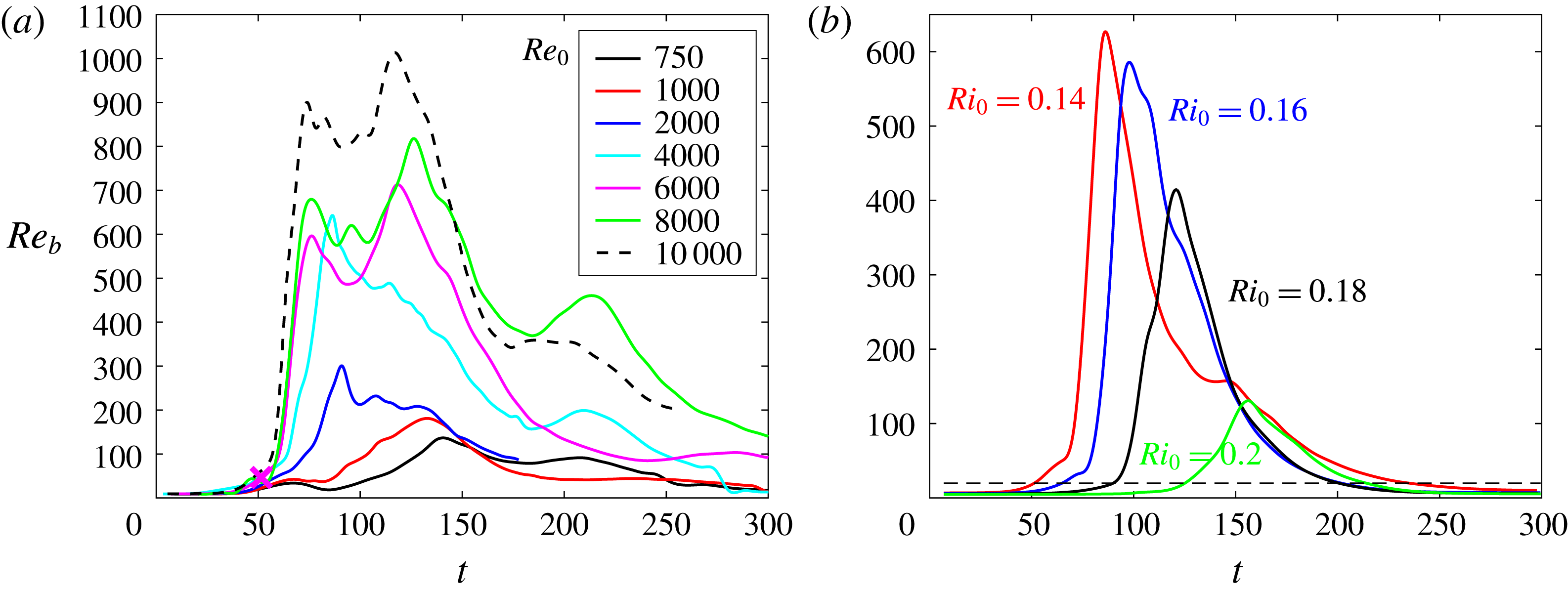
Time variation of buoyancy Reynolds number
 $Re_{b}$
for: (a) cases 4–10 of table 1, showing the variation with
 $Re_{0}$
for
 $Ri_{0}=0.12$
, all with vortex pairing allowed (noting that pairing is increasingly suppressed as
 $Re_{0}$
increases); (b) cases 11–14 of table 1, showing the variation with
 $Ri_{0}$
for
 $Re_{0}=6000$
for simulations with vortex pairing prohibited by design. Time is non-dimensionalized by the eddy turnover time scales
 $h/\unicode[STIX]{x0394}u$
where
 $\unicode[STIX]{x0394}u$
and
 $h$
are characteristic scales of the shear flow as defined in (2.1). The onset of fully developed turbulence for each case corresponds to the time
 $t_{3D}^{S}$
when the inherently three-dimensional turbulent kinetic energy peaks following a rapid growth during the transition to turbulence (see Caulfield & Peltier (Reference Caulfield and Peltier2000) and Mashayek et al. (Reference Mashayek, Caulfield and Peltier2013) for details). This time approximately coincides with the first peak of
 $L_{O}$
and also of
 $Re_{b}$
as defined here. The dashed line in (b) marks
 $Re_{b}=20$
which nominally marks the lower bound of stratified turbulence, even if not truly fully developed (see SM00 for a further discussion).

4.1 Time evolution of
$Re_{b}$

Figure 2 illustrates the time evolution of
 $Re_{b}$
for simulations with different
 $Re_{0}$
at
 $Ri_{0}=0.12$
(a) and for simulations with different
 $Ri_{0}$
at
 $Re_{0}=6000$
(b). The non-stationary nature of intermittent mixing by shear instability is clearly shown in the figure through the non-monotonic temporal evolution of
 $Re_{b}$
.
Figure 2(a) shows a qualitative change in the evolution of
 $Re_{b}$
for sufficiently large
 $Re_{0}\gtrsim 4000$
. At this intermediate
 $Ri_{0}$
, energetic time-dependent turbulence (i.e. with
 $Re_{b}>200$
) is maintained over a considerable fraction of the intermediate phase of the turbulence life cycle only for
 $Re_{0}=4000$
and larger. This is a critical difference from the simulations reported in SM00. It is apparent that any extrapolation on the basis of the results of lower
 $Re_{0}$
experiments or simulations (such as those reported in SM00) to geophysical flows which occur at much larger
 $Re$
must be treated with caution. Quantitatively, while
 $Re_{b}$
(defined in the fashion we use here) never exceeds 150 for
 $Re_{0}=750$
, (typical of the simulations reported in SM00)
 $Re_{b}$
remains above 200 for
 ${\sim}75\,\%$
of the turbulence life cycle for
 $Re_{0}=6000$
, when
 $Ri_{0}=0.12$
. The structure of the time evolution of
 $Re_{b}$
also exhibits qualitative differences between the simulations with lower
 $Re_{0}$
and higher
 $Re_{0}\gtrsim 4000$
. This observation is consistent with our hypothesis that a rich ‘zoo’ of secondary instabilities (only present at sufficiently high
 $Re_{0}$
) qualitatively modifies the subsequent turbulent evolution once those instabilities have broken down.
We now turn our attention to the dependence on
 $Ri_{0}$
of the behaviour of the flow at such sufficiently high
 $Re_{0}$
to sustain vigorous turbulence. We consider a range of
 $Ri_{0}$
for that turbulence to be non-trivially affected by stratification. As shown in figure 2(b), it is clear that this ‘energetic’ turbulence (i.e. with
 $Re_{b}>200$
) remains long lived (i.e. spans a significant portion of the turbulence life cycle) for all
 $Ri_{0}$
except
 $Ri_{0}=0.2$
. At this stage it is not clear why this qualitatively different behaviour occurs. One possibility is that the behaviour is associated with the Reynolds number being too small for this particular choice of
 $Ri_{0}$
, associated as it is with a primary instability with a growth rate so small that it may be adversely affected by the diffusion of the mean profiles, even at these Reynolds numbers. Alternatively, the behaviour may be due to the fact that the Richardson number is so close to the critical value of
 $0.25$
that the saturation amplitude of the nonlinear billow may so small that it leads to a qualitative change in the flow dynamics. Observational evidence (see for example the recent discussion of turbulence in the eastern equatorial Pacific by Smyth & Moum (Reference Smyth and Moum2013) and in the Romanche fracture zone by Van Haren et al. (Reference Van Haren, Gostiaux, Morozov and Tarakanov2014)) suggests that at the very large
 $Re_{0}$
characteristic of geophysical situations, instability and the ensuing turbulence onset soon after the Richardson number drops below
 $0.25$
, although it is extremely difficult to trace the dynamics precisely at the critical value, and so further investigation of shear instability for high
 $Re_{0}$
, and
 $Ri_{0}$
‘close’ in some sense to the critical value of
 $1/4$
is warranted.
Indeed, when considering geophysical relevance, it may be necessary to treat with caution the dynamics of flows with initially small values of
 $Ri_{0}$
, as it is not at all clear how such shear instability would be realizable in reality, as discussed above. And as mentioned earlier, the treatment of such low
 $Ri_{0}$
cases numerically requires particular care in terms of the choice of the spanwise extent of the domain to accommodate the braid instabilities which dominate turbulence transition in the limit of vanishing stratification. The importance of this issue is clearly connected to the rate at which the shear is diminished in a region of fixed background density stratification. If this time scale is sufficiently short, it is certainly at least plausible that a low Richardson number regime would be relevant.
4.2 Influence of Richardson number
The fundamental requirement that
 $Re_{0}$
be sufficiently large and (perhaps also that
 $Ri_{0}$
is a range where the flow is non-trivially affected by stratification) to capture geophysically realistic turbulent dynamics can also be observed in the way that the time evolution of the various length scales defined above vary in time for our different simulations. We are particularly interested in identifying what we believe should be ‘generic’ behaviour for high
 $Re_{0}-Ri_{0}$
flow, and what is affected by either
 $Re_{0}$
or
 $Ri_{0}$
being too ‘small’ in some sense. We showed in MCP13 that, in agreement with earlier theoretical predictions, for
 $Ri_{0}=0.16\sim 1/6$
mixing is most ‘efficient’ at sufficiently high Reynolds number. Here, efficiency is the fraction of energy available to turbulence that irreversibly increases the potential energy of the system. (We define efficiency precisely, and discuss this issue further in § 6.) This efficient mixing (at
 $Ri_{0}=0.16$
,
 $Re_{0}=6000$
,
 $Pr=1$
in MCP13) is due to an optimal excitation of secondary instabilities.
 $Ri=0.16$
is sufficiently high to induce a large number of baroclinically induced secondary instabilities yet it is not too high to suppress the turbulence. Therefore, here we choose to consider that flow simulation as the ‘canonical’ case.
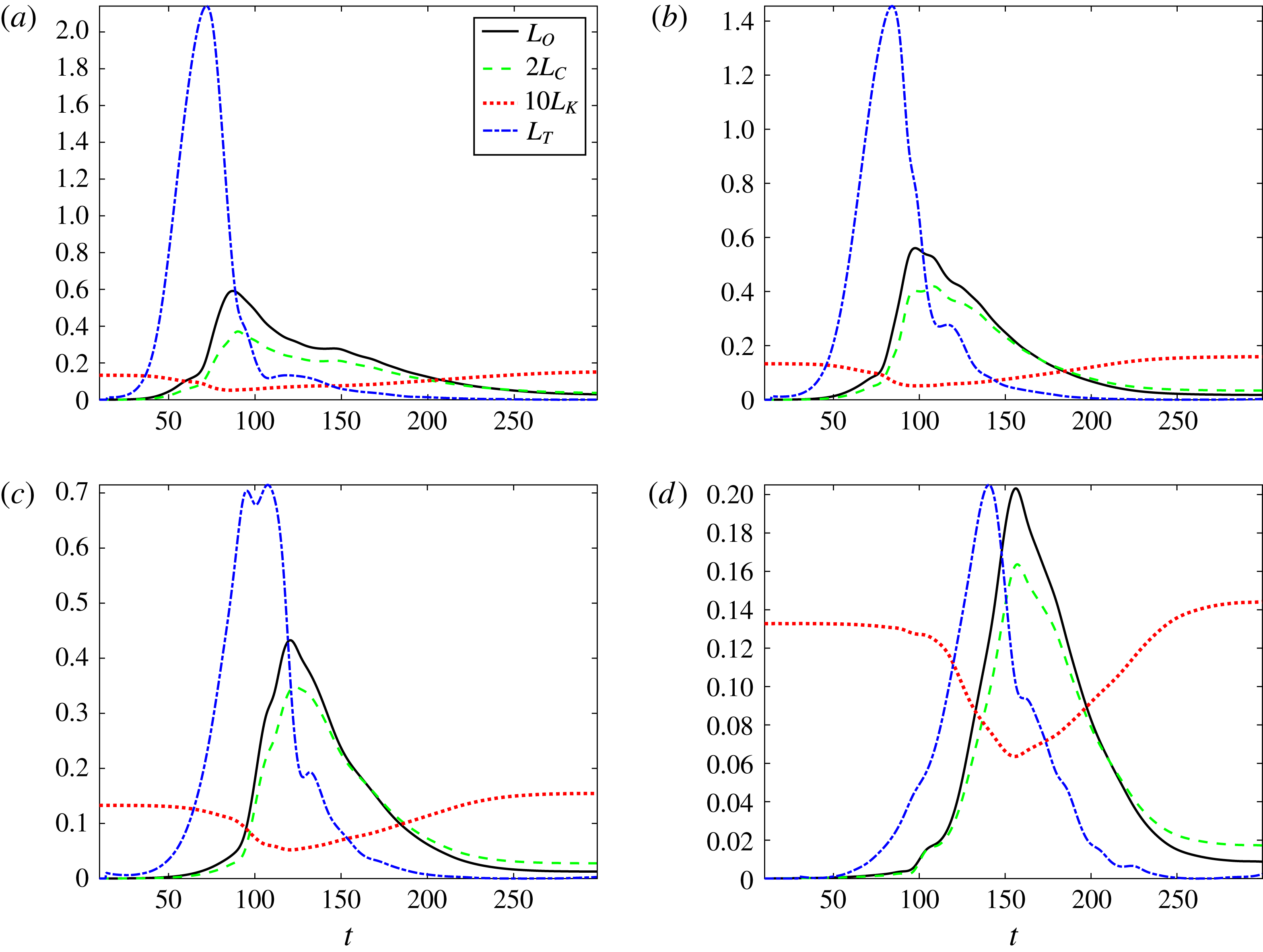
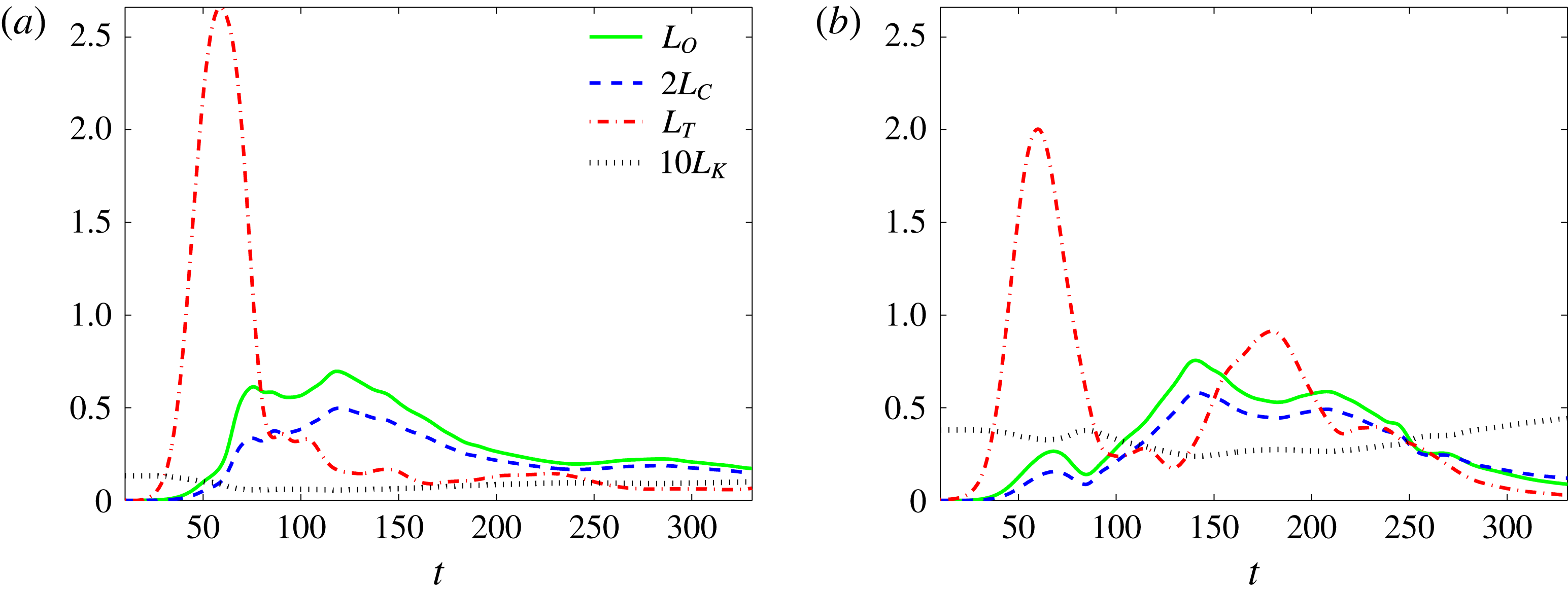
In figure 3(b), we plot the various length scales defined above for this simulation (case 12 in table 1). For completeness, we have also included the cases with
 $Ri_{0}=0.14$
,
 $Ri_{0}=0.18$
and
 $Ri_{0}=0.20$
. Similarly to figure 2(b), the evolution of the flow with
 $Ri_{0}=0.2$
is qualitatively different from the other three simulations.


Focusing on figure 3(b) for the simulation with
 $Ri_{0}=0.16$
, certain generic characteristics are as expected. Firstly, the Kolmogorov length scale
 $L_{K}$
(plotted with a dotted line) decreases rapidly at turbulence onset, and then recovers relatively slowly towards its laminar value as the turbulence decays after the turbulent kinetic energy saturates (i.e. peaks for the first time). Similarly, both the Ozmidov scale
 $L_{O}$
(plotted with a solid line) and the Corrsin scale
 $L_{C}$
(plotted with a dashed line) rapidly increase at transition, and then decay slowly towards their initial laminar values. Remembering that for clarity we are plotting
 $10L_{K}$
and
 $2L_{C}$
, it is clear that there is a wide scale separation between
 $L_{O}$
and
 $L_{K}$
as expected throughout the period (up to approximately
 $t\simeq 125$
) when
 $Re_{b}>200$
, demonstrating that there appears to be the possibility for a range of turbulent length scales which are unaffected by both viscosity and stratification.
Perhaps more surprising is the evolution of the Thorpe scale
 $L_{T}$
(plotted with a dashed-dotted line).
 $L_{T}$
grows during the initial roll up of the primary billow, and it grows substantially before turbulent motions onset, signalled by the marked drop of
 $L_{K}$
. After reaching a peak before the transition to turbulence,
 $L_{T}$
actually decreases rapidly during the period of most intense turbulent motion, indicative of vigorous irreversible, and inherently small-scale mixing, associated with the rich ‘zoo’ of secondary instabilities discussed in detail in Mashayek & Peltier (Reference Mashayek and Peltier2012a
,Reference Mashayek and Peltier
b
). We observe that
 $L_{T}>L_{O}$
during the transition to the turbulent phase of flow evolution while
 $L_{T}<L_{O}$
beyond the point of most intense turbulence (i.e. the time
 $t_{3D}^{S}$
with largest
 $L_{O}$
and smallest
 $L_{K}$
). Consistently with the recent detailed analysis of Mater & Venayagamoorthy (Reference Mater and Venayagamoorthy2014), this demonstrates that it is by no means appropriate to assume that
 $L_{O}$
is ‘the limiting size’ of overturns in strongly stratified turbulence during the turbulence growth phase. That
 $L_{T}>L_{O}$
in this phase actually suggests that the shear-driven turbulent mixing events considered here may be a candidate for creating the canonical layered structures within the previously proposed ‘strongly’ stratified turbulence scaling regime (see for example Brethouwer et al.
Reference Brethouwer, Billant, Lindborg and Chomaz2007).
Furthermore, the relative time dependence of the Thorpe scale and the Ozmidov scale is also of interest. Typically at these Reynolds numbers and Richardson numbers,
 $L_{T}$
‘flares’, in that it increases rapidly and in turn decreases rapidly before undergoing a slower decay once it has reached very small values.
 $L_{O}$
also increases rapidly, but effectively only when
 $L_{T}$
has reached its maximum. Interestingly, it appears that
 $L_{O}$
reaches its maximum (when the turbulence is most intense, in that
 ${\mathcal{E}}$
is largest) very close to the time when
 $L_{O}\approx L_{T}$
. Subsequently,
 $L_{O}$
‘burns’, in that it decreases at a noticeably slower rate than
 $L_{T}$
, suggesting a much more extended period of strong turbulence as opposed to strong overturning. We will further discuss the importance of the evolution of
 $L_{T}$
relative to
 $L_{O}$
in § 5.


Figure 3(d) shows that the behaviour is qualitatively different when
 $Ri_{0}$
is increased to
 $0.2$
(noting the dramatic reduction in the extent of the vertical axis with increase in
 $Ri_{0}$
). The turbulence is undoubtedly much less intense, with the Ozmidov scale peaking at a markedly reduced maximum value as
 $Ri_{0}$
increases. The relative time dependence of
 $L_{O}$
and
 $L_{T}$
is also qualitatively different. For
 $Ri_{0}=0.2$
, the Thorpe scale similarly peaks later and at lower values, and decays more slowly. These properties are indicative of a reduction in amplitude and delay and slowing of the primary overturns upon which turbulence grows and decays. They also imply a qualitatively different mixing dynamics from the other three cases shown. Indeed, unlike the
 $Ri_{0}=0.16$
case, at
 $Ri_{0}=0.2$
the time scale over which
 $L_{O}$
increases and that over which it subsequently decays are similar. Furthermore, the dissipation rate does not grow as much above its laminar value in this simulation compared to the
 $Ri_{0}=0.16$
simulation, and so there is not such a wide length scale separation between the Kolmogorov scale
 $L_{K}$
and the Ozmidov scale
 $L_{O}$
, indicating that both stratification and viscosity are likely to be modifying the turbulence dynamics substantially. This all constitutes evidence that the transition to turbulence is relatively weak in this flow, and so may well not be typical of the behaviour of intense geophysical turbulence at very high Reynolds number.
4.3 Influence of Reynolds number
We now investigate how the generic behaviour for the time dependence of the various length scales shown by the simulation with
 $Ri_{0}=0.16$
and
 $Re_{0}=6000$
in figure 3(b) is affected by variations in
 $Re_{0}$
and
 $Ri_{0}$
. Considering the effect of variations in
 $Re_{0}$
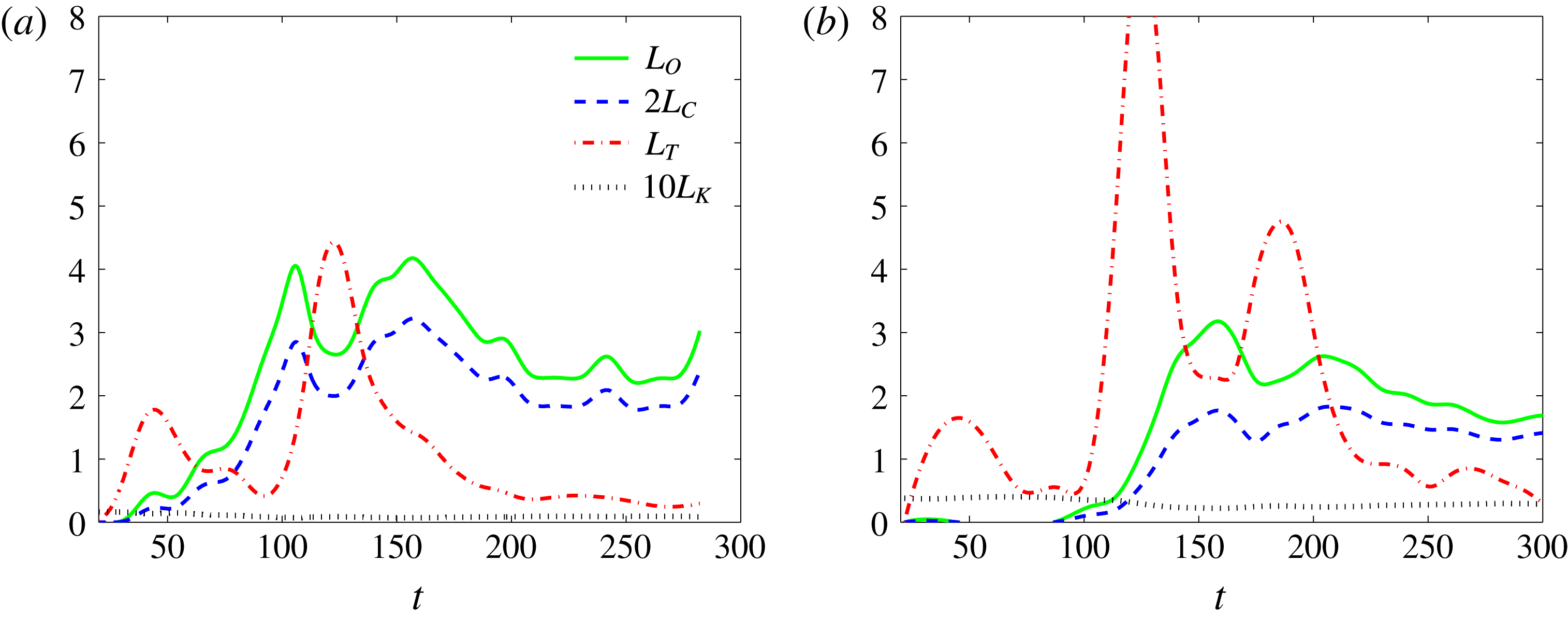
first, in figure 4 we plot the time evolution of the various length scales for simulations with
 $Re_{0}=6000$
and
 $750$
both with
 $Ri_{0}=0.12$
. The time dependence of the various length scales for the higher
 $Re_{0}$
is generally similar to the
 $Ri_{0}=0.16$
case shown in figure 3(b). There is once again a ‘flare’ in
 $L_{T}$
which appears to trigger a rapid increase in
 $L_{O}$
(and
 $L_{C}$
) followed by a slower decay towards laminar values. Indeed for this value of
 $Ri_{0}$
, there is essentially a period of relatively constant
 $L_{O}$
, indicative of sustained turbulence, and there is only a local (as opposed to global) maximum in
 $L_{O}$
as
 $L_{T}$
drops steeply indicating the break down of the primary billow related overturning.


Clearly, the lower Reynolds number simulation with
 $Re_{0}=750$
(of the same order as in the flows described in SM00) shown in figure 4(b) is qualitatively different. There is a substantially smaller-scale separation between
 $L_{O}$
and
 $L_{K}$
. Perhaps even more significantly, the temporal evolution of the Thorpe scale
 $L_{T}$
, both taken in isolation and relative to the time evolution of
 $L_{O}$
is also qualitatively different. The initial rapid decrease in
 $L_{T}$
is not associated with a peak in
 $L_{O}$
, with the most active turbulence occurring substantially later, principally because of the absence, at this Reynolds number of the ‘zoo’ of secondary instabilities which affects the simulations shown in figure 3. These are yet more data demonstrating that the evolution of length scales in a stratified shear flow changes markedly as
 $Re_{0}$
becomes sufficiently large. Therefore, we believe it is clearly necessary to consider flows with
 $Re_{0}\gtrsim 4000$
to investigate assumption IV discussed in the introduction, i.e. that there is a clear separation of scales between the background flow and the superposed (assumed) isotropic turbulence.
4.4 Summary of evolution of various scales
In summary, we wish to stress three key aspects of the results presented in this section. First, figures 2–5 show that the assumption of stationary stratified isotropic turbulence is very rarely satisfied, at best only in the energetic turbulence phase of flow for Reynolds numbers sufficiently large and close to a Richardson number ‘sweet spot’ at which mixing is optimal. According to MCP13, this sweet spot value of
 $Ri_{0}$
is defined by two competing effects:
 $Ri_{0}$
is sufficiently small so that turbulence is not completely suppressed by stratification and yet is sufficiently large for the flow to be replete with buoyancy-driven secondary and higher-order instabilities, which are only possible at sufficiently high
 $Re_{0}$
. From a length scale perspective this regime is characterized by the existence of a sufficiently wide separation between
 $L_{O}$
and
 $L_{K}$
. Importantly, these scales are turbulent length scales, by construction distinct from the length scales of the background mean flow. Second, over the entire parameter space we cover herein, the turbulence growth and decay periods of flow evolution, in which assumptions of isotropy and stationarity are clearly violated (as discussed in Smyth & Moum (Reference Smyth and Moum2000b
) and Mashayek & Peltier (Reference Mashayek and Peltier2013)), together constitute a large fraction of the typical turbulence life cycle. And finally, at sufficiently high
 $Re_{0}$
and
 $Ri_{0}$
in the correct range, there appears to be a typical or generic coupled time dependence of
 $L_{T}$
and
 $L_{O}$
.
 $L_{T}$
increases rapidly initially before undergoing a slow decay at very small values.
 $L_{O}$
, on the other hand, begins to grow rapidly when
 $L_{T}$
starts to decrease.
 $L_{O}$
reaches its maximum when it is
 ${\sim}L_{T}$
, and then decays noticeably more slowly than
 $L_{T}$
in the decay period of turbulence. In the next section we turn our attention to the ratio between these two length scales, in particular in this apparently generic regime for
 $Ri_{0}$
sufficiently large, but not too large, in flows at high
 $Re_{0}$
.
5
$L_{O}/L_{T}$
as a proxy for turbulence age and efficiency

As originally argued by Thorpe (Reference Thorpe1977), (see e.g. Scotti (Reference Scotti2015) for a detailed discussion) direct measurements of
 $L_{T}$
can be used to infer dissipation if
 $L_{T}$
can be shown to be a simple function of
 $L_{O}$
. In such a case, the dissipation rate can be calculated from the expression
 $$\begin{eqnarray}{\mathcal{E}}=R_{OT}^{2}L_{T}^{2}N^{3},\end{eqnarray}$$
where
 $$\begin{eqnarray}R_{OT}=\frac{L_{O}}{L_{T}}.\end{eqnarray}$$
Indeed, further progress can be achieved by making the further (though not always justified, see for example MCP13) assumption due to Osborn (Reference Osborn1980) that the buoyancy flux
 ${\mathcal{B}}$
, defined as
 $$\begin{eqnarray}{\mathcal{B}}=\frac{1}{V}\int \frac{g}{\unicode[STIX]{x1D70C}_{a}}\unicode[STIX]{x1D70C}w\,\text{d}v,\end{eqnarray}$$
can be linearly related to the dissipation rate
 ${\mathcal{E}}$
through a ‘universal’ turbulent flux coefficient
 $\unicode[STIX]{x1D6E4}$
(sometimes referred to as ‘mixing efficiency’). Using this assumption, a measurement of the Thorpe scale
 $L_{T}$
along with an appropriate buoyancy frequency
 $N$
are commonly used in the oceanographic research literature (see e.g. Dillon Reference Dillon1982, Thorpe Reference Thorpe2005, Kunze et al.
Reference Kunze, Firing, Hummon, Chereskin and Thurnherr2006) to estimate diapycnal eddy diffusivity through
 $$\begin{eqnarray}\unicode[STIX]{x1D705}_{T}\equiv \frac{{\mathcal{B}}}{N^{2}}=\frac{{\mathcal{B}}}{{\mathcal{E}}}\frac{{\mathcal{E}}}{N^{2}}=\unicode[STIX]{x1D6E4}R_{OT}^{2}L_{T}^{2}N.\end{eqnarray}$$
As discussed in detail by Mater et al. (Reference Mater, Venayagamoorthy, St. Laurent and Moum2015) and Scotti (Reference Scotti2015), estimates of the ratio
 $R_{OT}$
are very sensitive to the existence of large-scale overturnings within the flow, and since the ratio is squared in (5.4), uncertainty in its value has a marked effect on estimates of diapycnal diffusivity.
Furthermore, the time-dependent properties of the ratio
 $R_{OT}$
are also very important, as its particular value is often used to infer the ‘age’ of the turbulence involved in observed mixing events (Ivey & Imberger Reference Ivey and Imberger1991; SM00; Smyth et al.
Reference Smyth, Moum and Caldwell2001; Bouffard & Boegman Reference Bouffard and Boegman2013). Based on direct numerical simulations of Kelvin–Helmholtz billows at relatively low
 $Re_{0}$
, SM00 reported that
 $R_{OT}$
was typically observed to increase with time (see for example their figure 15) and argued in favour of the observational and entropy-based arguments of Wijesekera & Dillon (Reference Wijesekera and Dillon1997), that ‘older’ overturnings should be characterized by large values of
 $R_{OT}>1$
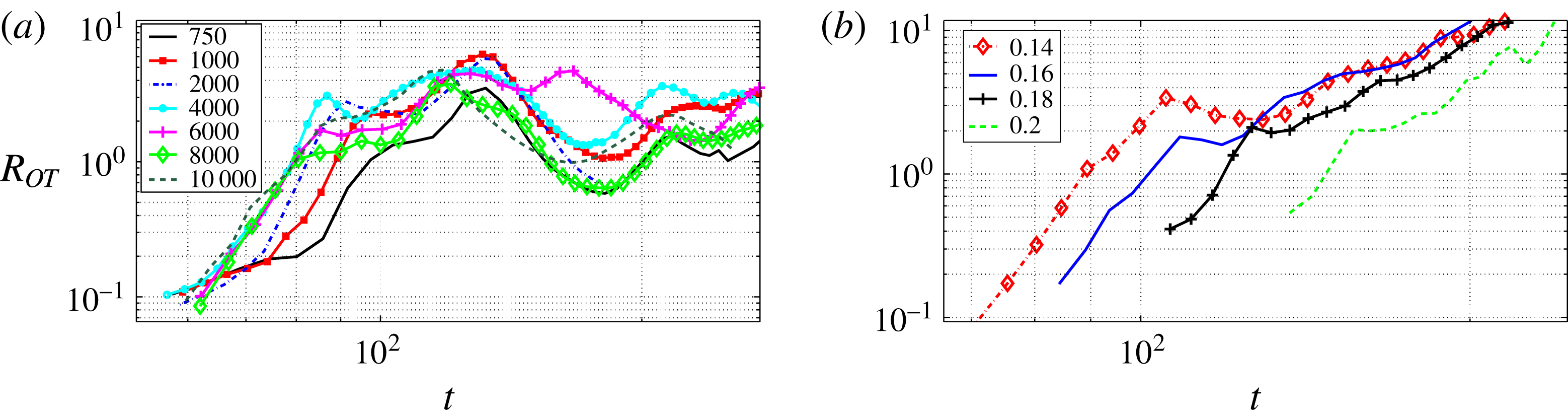
. We also observe the same qualitative trend as is shown in figure 6 which shows the time evolution of
 $R_{OT}$
for the same two groups of cases shown in figure 2. This is consistent with our ‘generic’ observation that, after its initial flare to very large values,
 $L_{T}$
decreases rapidly, to very small values, and in particular to values smaller than the more slowly decaying ‘burning’
 $L_{O}$
. For the single wavelength simulations in (b),
 $R_{OT}$
is indeed an increasing function of time. Conversely, for simulations shown in (a) which include two wavelengths of the primary Kelvin–Helmholtz instability and span an order of magnitude increase in
 $Re$
,
 $R_{OT}$
grows rapidly at transition, reaching a maximum around the time
 $t_{3D}^{S}$
when the inherently three-dimensional turbulence saturates, and then decays rapidly before showing a second oscillatory growth phase driven by variations in the rate of decay of
 $L_{T}$
and
 $L_{O}$
, due to the complicating merging dynamics. As already discussed, such merging dynamics is suppressed for flows with higher
 $Re_{0}$
, and so we do not believe that dynamics associated with merger of primary KHI billows is characteristic of geophysically relevant flows. This belief is reinforced by the fact that perturbations in real flows are highly unlikely to be ‘tuned’ to trigger merger events, and are typically much more broadband and noisy in structure, characterized by low amplitude or residual turbulent motions. Indeed, we are unaware of observations of merging billows in geophysical flows in the atmosphere and ocean, though there is much evidence of observations of long trains of individual billows.
Time evolution of the ratio
 $R_{OT}=L_{O}/L_{T}$
over the turbulent life cycle of flow for the same cases as those shown in figure 2: (a) shows results from simulations with
 $Ri_{0}=0.12$
and
 $750<Re_{0}<10^{4}$
(with pairing), while (b) shows results from simulations with
 $Re=6000$
and
 $0.12<Ri_{0}<0.2$
(with no pairing).

We note that while SM00 simulations were also conducted with streamwise extent which allowed for the development of two wavelengths of the primary instability, similarly to those shown in figure 6(a), their
 $R_{OT}$
evolution differs qualitatively and quantitatively from our results. They found a more monotonic increase in
 $R_{OT}$
with time during the decay period of turbulence. We believe that the difference between their results and ours is due to differences in the simulations’ initializations. SM00 initialized their simulations with non-trivial amplitude in the eigenfunction of pairing instability, leading to a relatively rapid pairing of KHI billows early in the simulation, which amounts to an initial pre-turbulent significant increase in
 $L_{T}$
, and subsequently a marked decrease in
 $L_{T}$
in the turbulent period of flow once vortices have paired. This apparently leads to a monotonic increase in
 $R_{OT}$
in the turbulent phase of the flow. On the other hand, our two wavelength simulations are not forced explicitly with the pairing mode eigenfunction and also are conducted at very high Reynolds number. As discussed above, flows with such higher
 $Re_{0}$
are associated both with a significant suppression of the pairing instability, and with fundamentally different character in the transition mechanisms (i.e. the full ‘zoo’ of secondary instabilities) and the intensity (quantified by the elevated values of
 $Re_{b}$
) of the ensuing turbulence. Perhaps unsurprisingly, such differences lead to a characteristically different
 $R_{OT}$
behaviour during the later stages of flows in which pairing (even if highly suppressed) manifests.
In summary, our results in this section suggest that the evolution of
 $R_{OT}$
in turbulence life cycles initiated by shear instability is very sensitive to details of the flow evolution such as the existence or lack thereof of an upscale cascade through pairing instability flow initialization. Therefore, it is at least plausible that the time dependence of
 $R_{OT}$
is likely to vary according to the degree of ambient or residual turbulence within a flow in which KHI billows develop, as is to be expected for a realistic geophysical flow. In spite of the relevance of
 $R_{OT}$
as a proxy for turbulence age, details of its evolution play an important role in characterizing the properties of the turbulence itself. Essentially,
 $L_{T}$
represents the vertical overturning scale of turbulence and so represents the large-scale stirring at which energy is being injected into the perturbation fields, while
 $L_{O}$
represents the largest eddies which are not strongly influenced by stratification, remembering that eddies smaller than
 $L_{O}$
and larger than
 $L_{C}$
are still affected by the ambient shear. Therefore, an optimal injection scale for the cascade of energy from larger-scale stirring to dissipation is expected. This corresponds to the stirring injection scale (
 $L_{T}$
) occurring at the largest scale not suppressed by stratification (
 $L_{O}$
), i.e. when
 $L_{O}\sim L_{T}$
. Precisely this behaviour was observed by Ivey & Imberger (Reference Ivey and Imberger1991), as this relationship corresponds to the optimal value for mixing of their turbulent Froude number
 $Fr_{T}=(L_{O}/L_{T})^{2/3}\simeq 1$
. As we see next, in this phase of flow evolution mixing is very efficient. Full discussion of the turbulence cascade and anisotropy in turbulence induced by KHI over a wide range Reynolds and Richardson numbers is provided in Mashayek & Peltier (Reference Mashayek and Peltier2013). Here we have built upon that study to connect it to the turbulent length scales discussed in this section and through that connection to mixing.
6 Implications for the quantification of mixing
The ‘mixing efficiency’, which we denote here by
 $\unicode[STIX]{x1D702}$
, is an important quantity which is commonly used for quantifying diapycnal mixing rates from observations of shear-induced turbulence in the ocean and atmosphere. We define
 $\unicode[STIX]{x1D702}$
within a Boussinesq framework as the ratio of the kinetic energy converted to potential energy irreversibly via a net irreversible vertical buoyancy flux, to the total irreversible conversion of kinetic energy to both potential energy and internal energy via viscous dissipation. This quantity is sometimes also referred to as the flux Richardson number, although the two quantities are not exactly the same at finite Reynolds numbers, as the denominator of the flux Richardson number is usually defined to be the production of turbulent kinetic energy (see Peltier & Caulfield (Reference Peltier and Caulfield2003), MCP13 and Rahmani, Lawrence & Seymour (Reference Rahmani, Lawrence and Seymour2014) for more discussion). The mixing efficiency is widely assumed to be
 $\unicode[STIX]{x1D702}\sim 0.15-0.2$
, equivalent to the canonical model due to Osborn (Reference Osborn1980) that the turbulent flux coefficient
 $\unicode[STIX]{x1D6E4}$
(as defined in (5.4)) is given by
 $\unicode[STIX]{x1D6E4}\simeq \unicode[STIX]{x1D702}/(1-\unicode[STIX]{x1D702})\leqslant 0.2$
despite the growing evidence demonstrating that it is highly variable in shear-induced mixing (see the recent results of MCP13 and Rahmani et al. (Reference Rahmani, Lawrence and Seymour2014)).
As discussed in more detail in Caulfield & Peltier (Reference Caulfield and Peltier2000) and Peltier & Caulfield (Reference Peltier and Caulfield2003), mixing efficiency can be considered to be a time-dependent quantity, and so it is natural to consider both instantaneous values
 $\unicode[STIX]{x1D702}_{i}(t)$
, and some appropriate cumulative mixing efficiency
 $\unicode[STIX]{x1D702}_{c}$
for a given mixing event. To calculate
 $\unicode[STIX]{x1D702}_{i}$
from our simulation results, we calculate the net instantaneous irreversible increase in the potential energy of the system, which represents diapycnal mixing
 ${\mathcal{M}}$
, and then define
 $$\begin{eqnarray}\unicode[STIX]{x1D702}_{i}=\frac{{\mathcal{M}}}{({\mathcal{M}}+{\mathcal{E}})},\end{eqnarray}$$
where
 ${\mathcal{E}}$
is the total dissipation rate as defined in (2.3), and
 ${\mathcal{M}}$
is determined using the sorting algorithm as initially described by Winters et al. (Reference Winters, Lombard, Riley and D’Asaro1995) and slightly modified in Caulfield & Peltier (Reference Caulfield and Peltier2000). More specifically,
 ${\mathcal{M}}$
is defined as the net change in the background potential energy of the system which may be calculated by an adiabatic sorting of the fluid parcels in the whole domain as was described earlier in calculation of the Thorpe scale. Since the background potential energy may only be increased, any change in it will correspond to diapycnal mixing in our set-up with periodic boundary conditions. We can also define a cumulative mixing efficiency
 $\unicode[STIX]{x1D702}_{c}$
as is now conventional as
 $$\begin{eqnarray}\unicode[STIX]{x1D702}_{c}=\frac{\displaystyle \int _{t_{s}}^{t_{e}}{\mathcal{M}}\,\text{d}t}{\displaystyle \int _{t_{s}}^{t_{e}}{\mathcal{M}}\,\text{d}t+\int _{t_{s}}^{t_{e}}{\mathcal{E}}\,\text{d}t},\end{eqnarray}$$
for appropriately chosen start time
 $t_{s}$
and end time
 $t_{e}$
. We set
 $t_{s}=t_{3D}^{S}$
, and
 $t_{e}$
to be the end of the simulation (when the flows have typically relaminarized) to define
 $\unicode[STIX]{x1D702}_{c}^{3D}$
, which we list in table 1 for each of the simulations. (See Mashayek et al. (Reference Mashayek, Caulfield and Peltier2013) for more discussion.) In what follows we divide the turbulent life cycle of each simulation into a number of intervals and average
 $\unicode[STIX]{x1D702}$
over each period to obtain a locally averaged efficiency
 $\unicode[STIX]{x1D702}_{a}$
for each interval. Each period is set to be of 10 eddy turnover time scales (defined as
 $h/\unicode[STIX]{x0394}u$
where
 $\unicode[STIX]{x0394}u$
and
 $h$
are characteristic scales of the shear flow as defined in (2.1)), keeping in mind that the turbulent life cycle of the simulations in table 1 (nominally defined as the period over which
 $20<Re_{b}$
) typically extends over 200 to 400 turnover time scales.
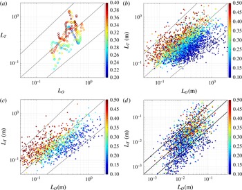
In figure 7(a) we show the results of calculations for simulations 6–14 of table 1. This subset includes cases with
 $Re_{0}$
sufficiently high to represent sustained turbulence for a considerable fraction of flow evolution, and with
 $Ri_{0}$
sufficiently large for the behaviour to share the key ‘generic’ characteristics of the simulation with
 $Ri_{0}=0.16$
as discussed above. To connect the interpretation of evolution of efficiency of mixing in the simulations with the time dependence of the various length scales as described in the previous section, figure 7 shows a scatter plot of
 $L_{T}$
versus
 $L_{O}$
, with the symbol colours representing
 $\unicode[STIX]{x1D702}_{a}$
. The lines in the figure represent
 $L_{T}=L_{O}$
,
 $L_{T}=4\times L_{T}$
and
 $L_{T}=0.25\times L_{O}$
, the latter two providing bounds on the
 $L_{O}/L_{T}$
ratio in observations (see Thorpe Reference Thorpe2005, for discussion and references). As discussed earlier, symbols for which
 $L_{T}>L_{O}$
correspond to the period in flow evolution in which eddies (of scales
 $L\leqslant L_{O}$
) associated with secondary instabilities grow rapidly and efficiently within the primary overturn, while symbols with
 $L_{T}<L_{O}$
correspond to the final period of the flow evolution when the turbulence is decaying and stirring is suppressed by ambient stratification. It is apparent that mixing is most efficient during the earlier period, particularly when
 $L_{T}\sim L_{O}$
, (precisely as assumed by Ivey & Imberger (Reference Ivey and Imberger1991)) since the inertial subrange is very efficiently energized at the upper bound (stirring scale) by the available potential energy reservoir stored in the primary overturn. As stirring by large eddies becomes suppressed by stratification in the later period of turbulence, mixing is less efficient. Thus, the high efficiency of mixing at
 $L_{O}\sim L_{T}$
appears to be a direct consequence of the nature of turbulence induced by shear instability at high Reynolds number. Importantly, this violates assumption IV as described in the introduction, because the length scale of the overturning is most definitely not widely separated from the important length scales of the turbulent motions.
Scatter plot of
 $L_{T}$
versus
 $L_{O}$
from DNS (a) and observations (b,c,d). (a) From DNS cases 6–14 of table 1. (b) From FLX91 oceanic dataset collected
 ${\sim}1000~\text{km}$
off the coast of northern California. (c) From the TIWE oceanic dataset collected at the equator at
 $140\,^{\circ }\text{W}$
. (d) From lake observations made at thermocline depth in Lake Erie in 2008–2009. More information about the sources of these datasets are provided in appendix A. The lines in each panel represent
 $L_{T}=L_{O}$
,
 $L_{T}=4\times L_{O}$
and
 $L_{T}=0.25\times L_{O}$
. Symbol colours and colour bars represent mixing efficiency
 $\unicode[STIX]{x1D702}_{a}$
. Note that the axes in (a) are normalized by
 $L_{sc}$
as was the case throughout this paper while in (b–d) they are in units of metres.

Furthermore, since this most efficient mixing occurs when
 $L_{O}\leqslant L_{T}$
, which is also in the build up to the instant when both
 $L_{O}$
and
 $Re_{b}$
are maximum, the actual total amount of mixing in the build up to
 $L_{O}\sim L_{T}$
is also maximized. In other words, since
 $\unicode[STIX]{x1D6E4}\simeq \unicode[STIX]{x1D702}_{a}/((1-\unicode[STIX]{x1D702}_{a}))$
(for caveats see MP13 and Salehipour & Peltier (Reference Salehipour and Peltier2015)), the observation that
 $\unicode[STIX]{x1D702}_{a}$
is maximum when
 $Re_{b}$
is maximum strongly suggests that the turbulent diffusivity
 $\unicode[STIX]{x1D705}_{T}$
is also maximum at that time, since using (2.2) and (5.4) we have,
 $$\begin{eqnarray}\unicode[STIX]{x1D705}_{T}=\unicode[STIX]{x1D6E4}\frac{{\mathcal{E}}}{N^{2}}\simeq \unicode[STIX]{x1D708}\frac{\unicode[STIX]{x1D702}_{a}}{(1-\unicode[STIX]{x1D702}_{a})}Re_{b}.\end{eqnarray}$$
This suggests that the flow at this time is so organized as to maximize the amount of vertical mass flux, because of the combined effects of the turbulence being most intense (i.e. with largest
 $Re_{b}$
) and most efficient (i.e. with largest
 $\unicode[STIX]{x1D702}_{a}$
and hence largest
 $\unicode[STIX]{x1D6E4}$
).
The above description of the dependence of mixing on the temporal evolution of
 $L_{O}$
and
 $L_{T}$
was based on simulations of Kelvin–Helmholtz instabilities that form the basis of our work. So, it is legitimate to question their generality insofar as the much more dynamically diverse ocean mixing process is concerned. However, we conjecture that the observation that the existence of distinct overturns provides sufficient available potential energy that can feed efficient turbulent mixing is not a special phenomenon only occurring in KHI flows, but is a more generic property of high Reynolds number stratified mixing processes, triggered by a wider range of mechanisms, including other shear instabilities, hydraulically controlled flows, or breaking internal waves. Clearly further work is warranted to test this conjecture by investigating the mixing associated with these wider range of mechanisms.
To explore this further, figure 7(b–d) shows similar scatter plots to that from our DNS in (a). The data for panels (b,c) come from observations made in the thermocline of the ocean while the data for panel (d) come from one of the great lakes (Lake Erie) in the United States. Mixing in these natural environments is induced by a mixture of dynamical processes including vertically propagating internal waves and shear instabilities of different types. Panels (b–d) share the same pattern with panel (a) in that mixing efficiency is larger for
 $L_{T}>L_{O}$
, further highlighting the role of natural overturns in determining the efficiency of mixing.
We acknowledge that our simulations are highly idealized and that the observational data used in figure 7 are based on a number of crude assumptions made for practical reasons; importantly, the calculation of mixing efficiency from data is difficult and involves large inaccuracies. Furthermore, there seem to be some systematic and as yet unexplained differences between how data are skewed about the
 $L_{O}=L_{T}$
line in the four panels. For example, the lake data in figure 7(d) appear to be more qualitatively similar to the numerical data in figure 7(a) than to the two oceanographic datasets in figure 7(b,c). Nevertheless, our main point here is neither dependent on the actual value of mixing efficiency nor is it sensitive to the above-mentioned inaccuracies and idealizations. Essentially, as long as distinct overturns exist throughout turbulence evolution, they play a non-negligible role in determining the efficiency of mixing. This point is one of the main messages of this paper.
We stress that this point is important for two reasons. First, as discussed earlier, conventional parameterization schemes are based on assumptions which are typically better satisfied during the turbulence decay period (i.e. towards the left in each panel). Second, the majority of studies of DNS of shear instabilities have focused on the decay period by filtering the earlier period based on the (at times implied) justification that the early period does not conform to a plausible ‘ocean turbulence regime’, assumed by (for example) Osborn (Reference Osborn1980) to be well modelled as stationary isotropic turbulence where the steady turbulence production is balanced by an isotropic dissipation rate and a relatively small (positive) buoyancy flux. In combination, these assumptions appear to have led to a circular argument for filtering the part of simulations that does not fit the parameterizations even though the simulations are carried out for the very purpose of improving the parameterizations. It was shown in Mashayek & Peltier (Reference Mashayek and Peltier2013) that in direct numerical simulations of shear instabilities, the early period of turbulence makes a non-negligible contribution to the net buoyancy flux over a turbulence life cycle. Furthermore, the analysis of Smyth et al. (Reference Smyth, Moum and Caldwell2001) showed that the
 $L_{O}<L_{T}$
patches in data used in figure 7 make a large contribution to net mixing as well. So, as long as large overturns exist, the contribution of the earlier period of turbulence in which distinct overturns and superimposed turbulence co-exist needs to be taken into account in both parameterization schemes and in analysis of numerical simulations. Of course, it is important to remember that in the observational data there is no ‘time stamp’, in that unlike the simulation data there is no way to follow the time evolution of an individual mixing event. However, the observational data are at least consistent with the idea that
 $L_{O}<L_{T}$
patches are associated with vigorous overturnings that will subsequently lead to increased turbulent mixing, and hence
 $L_{O}$
remaining larger for a longer time than
 $L_{T}$
, i.e. that
 $L_{T}$
‘flares’ while
 $L_{O}$
‘burns’, analogously to our simulations.
The contribution of overturns is partially filtered in conventional parameterizations by assumptions of isotropic stationary small-scale turbulence existing at a scale distinctly separated from that of the background flow. It has also often been left out of analysis of DNS data for several reasons. Distinct overturns observed in early DNS are often thought to be artefacts of the low
 $Re$
idealized nature of such simulations (Peltier & Caulfield Reference Peltier and Caulfield2003) and furthermore, the argument has been advanced that the later-time turbulence is more likely to be representative of stratified turbulence events, not necessarily generated by flows initially strongly unstable to KHI billows (Salehipour & Peltier Reference Salehipour and Peltier2015; Salehipour et al.
Reference Salehipour, Peltier and Mashayek2015, Reference Salehipour, Caulfield and Peltier2016a
).
However, recent direct numerical simulations at high Reynolds number and numerous recent observations of deep ocean turbulence have clearly shown that distinct overturns not only can exist, but in fact are typical in strong mixing zones. It almost appears as if the flow is trying to maximize efficiency of mixing by providing an efficient energy pathway into turbulence by stirring and storage of potential energy through overturns. Recent field experiments focused on abyssal ocean mixing (where mixing plays a key role in closure of abyssal branch of ocean meridional overturning circulation) have all found turbulence to be induced by continuous excitations of large overturns scaling from a few metres up to 500 metres (Ferron et al. Reference Ferron, Mercier, Speer, Gargett and Polzin1998; Frants et al. Reference Frants, Damerell, Gille, Heywood, MacKinnon and Sprintall2013; Mater et al. Reference Mater, Venayagamoorthy, St. Laurent and Moum2015; Voet et al. Reference Voet, Girton, Alford, Carter, Klymak and Mickett2015). Thus, we conjecture that underestimation of mixing due to partial neglect of the role of overturns may well obscure significantly the apparent tendency of turbulence to maximize its mixing efficiency through such overturns.
We think it useful to reiterate our reasoning for not adding data from low
 $Ri_{0}$
cases to figure 7(a). Since the growth rate of the primary Kelvin–Helmholtz instability is a monotonically decreasing function of
 $Ri_{0}$
, it is tempting to decrease
 $Ri_{0}$
to reduce computational cost since the simulation will in principle need to be conducted for a shorter time interval for a given computational domain. However, this reduction in computational cost is likely to be swamped by the need to consider larger computational domains, to capture at least some of the merging dynamics, which inevitably introduces large-scale stirring. Furthermore, as discussed earlier, the spanwise extent of the domain may possibly need to be expanded to host braid instabilities dominating turbulence transition in the weak stratification limit. Suppressing the stirring associated with such large-scale streamwise and spanwise secondary instabilities inevitably reduces the amount of mixing which apparently occurs in a simulation in a smaller domain. Indeed, it is entirely possible that as
 $Re$
is increased, the relative intensity of secondary instabilities at such smaller
 $Ri_{0}$
may change in as yet not fully understood ways. Since the extent to which such considerations can influence our low
 $Ri$
direct numerical simulations has not been fully explored due to computational limitations, we refrain from presenting quantitative arguments about mixing properties of such simulations. A detailed discussion of the potentially misleading nature (at least insofar as geophysically relevant mixing is concerned) of low
 $Ri$
numerical simulations designed to produce high
 $Re_{b}$
during the flow evolution is presented in Bartello & Tobias (Reference Bartello and Tobias2013).
In summary, while a number of studies have attempted to parameterize mixing efficiency as a function of
 $Re_{b}$
or in terms of
 $L_{O}/L_{T}$
(see Bouffard & Boegman Reference Bouffard and Boegman2013, for a review), we find neither approach to be sufficient. Essentially,
 $Re_{b}$
includes information concerning
 $L_{O}$
and
 $L_{K}$
, while the ratio
 $L_{O}/L_{T}$
clearly lacks explicit information about
 $L_{K}$
. As demonstrated here, knowledge of all three scales is needed for characterizing shear-driven stratified turbulent mixing, and so we believe that the large discrepancies between various attempts at parameterizing mixing based on either
 $Re_{b}$
or
 $L_{O}/L_{T}$
are due to a lack of such additional knowledge. Despite such discrepancies, we have demonstrated here that the specific role in the efficiency of mixing of the large overturns themselves is significant, corresponding to a non-negligible portion of the turbulence life cycle in which
 $L_{T}>L_{O}$
. The role of overturns also appears to be similar for the data from our simulations and for ocean and lake data. Such efficient mixing is inherently associated with the presence of large-scale overturns. The clearly more efficient mixing associated with such overturns is systematically left out of conventional parameterizations (based around the classical model of Osborn (Reference Osborn1980) assuming
 $\unicode[STIX]{x1D6E4}\leqslant 0.2$
) that are used to infer mixing rates from observations.
7 Discussion
We have analysed a sequence of direct numerical simulations of stratified turbulent mixing events driven by classical shear instability, focusing on a consideration of the relative time dependence of various natural length scales of turbulence and the implications of aspects of this relative time dependence for the irreversible vertical mixing of density. Our analyses demonstrate that for ‘small’ stratification, the turbulence and ensuing mixing is dominated by large density overturns and pairing interactions and so any parameterization based on the assumptions of stationary fully developed isotropic turbulence does not hold, in the specific sense that the assumptions I–IV mentioned in the introduction do not hold. It is important to note, however, that there is evidence that the upscale cascade due to pairing instability may well be suppressed at sufficiently high (perhaps more geophysically relevant) Reynolds numbers, a regime that we have been unable to access with the currently employed suite of direct numerical simulation analyses, although there is always the possibility that other processes may become more important as
 $Re$
increases markedly.
Conversely, for ‘large’ stratification with minimum Richardson number sufficiently close to the critical Miles–Howard value of
 $1/4$
, mixing is highly time dependent and a prolonged intermediate period of isotropic stationary turbulence is absent, corresponding to the break down of assumptions II–III mentioned in the introduction. In this regime, the scale separation between
 $L_{O}$
and
 $L_{K}$
is relatively narrow and turbulence is greatly influenced by the suppressing influence of stratification. However, it is unclear whether this behaviour is affected by finite Reynolds number effects, as the growth rate of the primary instability is so small that diffusion of the background flow may be affecting adversely the maximum saturated amplitude of the primary instability, in as yet poorly understood ways.
We argue that the behaviour at slightly smaller intermediate levels of stratification, where pairing events are suppressed, and yet the primary instability is sufficiently vigorous to allow for the onset of a large ‘zoo’ of secondary instabilities which trigger energetic turbulence leads to a ‘generic’ shear-driven stratified mixing behaviour. Specifically, this generic behaviour exhibits a very efficient turbulence downscale cascade through the inertial subrange when
 $L_{T}>L_{O}$
because of the large pool of potential energy available to sub-
 $L_{O}$
eddies due to the large initial overturn, whose vertical scale is characterized by
 $L_{T}$
. This translates into high mixing efficiency, which peaks when
 $L_{T}\sim L_{O}$
as at that particular time stirring becomes ‘optimal’ since it is occurring at the largest energy injection scale possible that is not suppressed by stratification. Although we refer to this behaviour as ‘generic’, it is important to note that the existence of the early
 $L_{T}\geqslant L_{O}$
regime, particularly associated with relatively large-scale overturnings, is not guaranteed in the evolution of all shear-unstable flows and is likely to be environment dependent. For example, KHI billows in an energetic estuary have been shown not to evolve distinct vorticity cores which store potential energy with the effective
 $L_{T}$
being relatively small (Geyer et al.
Reference Geyer, Lavery, Scully and Trowbridge2010) while other forms of shear instability (such as the Holmboe instability, see Salehipour et al. (Reference Salehipour, Caulfield and Peltier2016a
) for further details) are not characterized by large overturns, but rather drive mixing principally through ‘scouring’ (Woods et al.
Reference Woods, Caulfield, Landel and Kuesters2010). However, energetic overturning billows similar in structure to those described here have been observed growing on low-frequency internal tides in the abyssal ocean (van Haren & Gostiaux Reference van Haren and Gostiaux2010, Reference van Haren and Gostiaux2012), in deep ocean fracture zones (Van Haren et al.
Reference Van Haren, Gostiaux, Morozov and Tarakanov2014) and in the thermocline (Thorpe Reference Thorpe2005). And as we discussed earlier, several deep ocean field programs have repeatedly shown that abyssal diapycnal mixing is facilitated through large overturns which can range in size from a few to hundreds of metres (Ferron et al.
Reference Ferron, Mercier, Speer, Gargett and Polzin1998; Frants et al.
Reference Frants, Damerell, Gille, Heywood, MacKinnon and Sprintall2013; Mater et al.
Reference Mater, Venayagamoorthy, St. Laurent and Moum2015; Voet et al.
Reference Voet, Girton, Alford, Carter, Klymak and Mickett2015).
We show not only that mixing efficiency depends upon
 $L_{O}/L_{T}$
, but that it also depends on the scale separation between
 $L_{O}$
and
 $L_{K}$
, i.e. the width of the inertial subrange of turbulence, or equivalently the magnitude of the buoyancy Reynolds number
 $Re_{b}$
. Fundamentally, the key constituents of efficient and vigorous mixing are that
 $L_{T}\gtrsim L_{O}$
and
 $L_{O}/L_{K}$
is sufficiently large. Therefore, we argue that parameterization of mixing efficiency based on
 $Re_{b}=(L_{O}/L_{K})^{4/3}$
alone is insufficient as it misses the important relative properties of
 $L_{T}$
and
 $L_{O}$
, while parameterization based on
 $L_{T}/L_{O}$
alone is also insufficient as it misses the
 $Re_{b}$
contribution. We conjecture that the key physics of both an optimal injection scale and a wide inertial subrange are required. Such flows also violate assumption IV presented in the introduction, as there is not a large-scale separation between the external forcing (characterized by
 $L_{T}$
) and the turbulence (characterized at the largest scale by
 $L_{O}$
).
It is important to note that while some parameterization schemes for inferring mixing from observations assume isotropy of the turbulence (Osborn & Cox Reference Osborn and Cox1972; Osborn Reference Osborn1980), a large number of observational studies which measure both
 $L_{T}$
and
 $L_{O}$
suggest that
 $L_{T}\geqslant L_{O}$
, implying non-negligible anisotropy (Dillon Reference Dillon1982; Crawford Reference Crawford1986; Ferron et al.
Reference Ferron, Mercier, Speer, Gargett and Polzin1998; Smyth et al.
Reference Smyth, Moum and Caldwell2001; Mater et al.
Reference Mater, Venayagamoorthy, St. Laurent and Moum2015). In fact,
 $L_{O}/L_{T}=0.8$
is a standard choice made to obtain the dissipation rate
 ${\mathcal{E}}$
from
 $L_{T}$
calculated based upon fine structure measurements of temperature or salinity and when microstructure estimates are unavailable (see for example Waterhouse et al.
Reference Waterhouse, Mackinnon, Nash, Alford, Kunze, Simmons, Polzin, St Laurent, Sun and Pinkel2014). It is particularly important to note that while
 $0.8$
might be a reasonable turbulence life cycle mean for
 $L_{O}/L_{T}$
, the fact that the ratio is likely much higher during the intermediate period of flow evolution in which buoyancy flux is maximized (as a result of the coexistence of distinct overturns upon which turbulence is superimposed) implies an underestimation of mixing when a constant ratio is used in the fine-scale parameterization based on the Thorpe scale. Just how large this underestimation is, and how parameterizations may be modified to capture the mixing associated with large-scale overturnings, are both topics of ongoing research (see e.g. Mashayek et al.
Reference Mashayek, Salehipour, Bouffard, Caulfield, Ferrari, Nikurashin, Peltier and Smyth2017).
Acknowledgements
A.M. acknowledges support from a David Crighton Fellowship from the Department of Applied Mathematics and Theoretical Physics, University of Cambridge, where this research was initiated and support from an NSERC PDF award. The research of W.R.P. in Toronto is supported by NSERC Discovery grant A9627. The research activity of C.P.C. is supported by EPSRC Programme grant EP/K034529/1 entitled ‘Mathematical Underpinnings of Stratified Turbulence’. We thank W. D. Smyth and J. N. Moum for sharing the ocean data and D. Bouffard for sharing the lake data used in figure 6. Data used to construct figures 2–7 are available at https://doi.org/10.17863/CAM.10527. We also thank three anonymous reviewers whose insightful and constructive comments have led to a substantial improvement in this paper.
Appendix A. Datasets
The first two oceanic datasets employed for construction of figure 7(b,c) were introduced in Smyth et al. (Reference Smyth, Moum and Caldwell2001). Panel (b) corresponds to the FLX91 dataset which was collected during the FLUX STATS cruise in 1991 approximately 1000 km off the coast of northern California (Moum Reference Moum1996). The dataset used in (c) is from the Tropical Instability Wave Experiment (TIWE) and was collected at the equator at
 $140\,^{\circ }\text{W}$
in 1991 (Lien et al.
Reference Lien, Caldwell, Gregg and Moum1995). The dataset used in the construction of (d) in figure 7 was introduced in Bouffard & Boegman (Reference Bouffard and Boegman2013) and corresponds to observations made at thermocline depth in Lake Erie during the summers of 2008–2009.
Appendix B.
$L_{T}^{3D}$
versus
$L_{T}$
and caveats for oceanographic implications


Our focus in this paper was upon the role of overturns on turbulent mixing in geophysical shear flows, and more specifically a focus on conditions relevant to oceans and lakes. The main message of the paper was based on analysis of energy conversion from the mean kinetic energy (provided by large-scale forcing from a variety of sources including estuarine exchanges, low-frequency internal wave shear etc.) to available potential energy and from there to a cascade of overturns that take energy down to scales at which diapycnal mixing and viscous dissipation occur. Our main message is that the existence of an intermediate non-trivial overturning scale between the mean background flow and small-scale turbulence allows for an efficient energy pathway into diapycnal mixing by providing additional stirring and filamentation, thereby enhancing the efficiency of mixing. To convey this message and its sensitivity to variations in Reynolds and Richardson numbers, we employ a definition of the Thorpe scale, referred to as
 $L_{T}^{3D}$
, which is only really practical in three-dimensional numerical modelling. In this appendix we provide a number of caveats highlighting the differences between this measure of overturning and the one-dimensional classical Thorpe scale
 $L_{T}$
, which for practical limitations is used to infer mixing rates and is constructed from localized profile measurements in oceanic and lake environments. We emphasize that the main message of our work does not depend on the differences we highlight here. Indeed, the importance of taking into account the existence of such an intermediate overturning scale in parameterization of mixing in the oceanographic context has already been pointed out by Kunze (Reference Kunze2014). Our research provides a further fluid mechanical basis for such an argument. Furthermore, we note that while
 $L_{T}^{3D}$
cannot be obtained from observations, certain observational techniques such as those employed by Geyer et al. (Reference Geyer, Lavery, Scully and Trowbridge2010) provide a series of parallel profiles measured through turbulent wave trains. Such measurements can provide a means for constructing a
 $L_{T}^{2D}$
to fill in the gap between our study and the majority of observational studies based on one-dimensional
 $L_{T}$
.
While physically meaningful and suitable for diagnosis from numerical models, the root mean square three-dimensional Thorpe scale
 $L_{T}^{3D}$
obtained in this work by full three-dimensional sorting of the density field has important differences from the one-dimensional
 $L_{T}$
. Importantly, while the
 $L_{T}^{3D}$
can be non-zero in the presence of a propagating wave without any overturns, or even in the presence of an overturn riding on a background low-frequency internal wave, just to take two examples, the one-dimensional
 $L_{T}$
is only non-zero in the presence of true overturns. In our study, however, we have only considered flows strongly susceptible to the Kelvin–Helmholtz instability, which overturns upon initiation of (exponential) growth. Thus, this caveat (that
 $L_{T}^{3D}$
may return a ‘false positive’ of overturning) does not concern our specific application and so we are safe in using
 $L_{T}^{3D}$
as a surrogate for an overturning scale.
A close comparison of the three-dimensional and one-dimensional Thorpe scales was provided by SM00. They found that the three-dimensional scale exceeds the one-dimensional scale in the decay period of turbulence (induced by shear instability) when the Thorpe scale is small. The generality of this argument in a more complex environment in which vertical displacements are not entirely or even partially driven by overturning instabilities is unclear, especially noting that (as mentioned above) there are scenarios in which the three-dimensional displacement scale might be non-zero while the one-dimensional scale remains zero due to lack of overturning. Nevertheless, this difference is not of central importance in the class of flows which we are considering, since in the case of shear instability both scales are measures of the physical overturning scale, are not too different during the most energetic period of turbulence over which most of the contribution to the net buoyancy flux is made, and can be employed to provide a measure of the width of the spectral gap between the energy injection scale and the upper bound of the inertial subrange.
However, during the decay period of turbulence, the one-dimensional Thorpe scale is smaller than the three-dimensional Thorpe scale. Therefore, it is to be expected that
 $L_{O}/L_{T}$
grows larger with time than
 $L_{O}/L_{T}^{3D}$
. This has implications for our discussion of figure 6: while
 $L_{O}/L_{T}$
is likely a monotonically increasing function of time and hence might be more naturally treated as a proxy for turbulence age,
 $L_{O}/L_{T}^{3D}$
is not as clear a proxy. From a physical point of view, the difference between
 $L_{O}/L_{T}^{3D}$
and
 $L_{O}/L_{T}$
in the decay period of turbulence in a flow susceptible to Kelvin–Helmholtz instability is testament to the shortcomings of
 $L_{T}$
in capturing the totality of the significant flow physics. A close look at figure 6(a) (which represents cases that, unlike those in (b), allow for interactions between adjacent billows) reveals that the ratio
 $R_{OT}=L_{O}/L_{T}^{3D}$
remains
 $O(1)$
during the decay period of the turbulence. This suggests that as turbulence decays and the energy injecting eddies shrink, so does the Ozmidov scale accordingly. This further suggests that the eddies associated with the dominant energetic injection, which are decaying in amplitude and magnitude since the turbulent kinetic energy and the Thorpe scale are both dropping, may also be thought of as the largest eddies not yet suppressed by turbulence. Conversely,
 $R_{OT}\equiv L_{O}/L_{T}$
(based on the one-dimensional Thorpe scale) suggests that
 $L_{T}$
can become much smaller than
 $L_{O}$
in this period, which implies that energy injection eddies are much smaller than the maximum size which is not suppressed by stratification, which seems somewhat inconsistent from a physical perspective.
As we discussed above, despite these subtle differences, there are at least two further leading-order issues with this proxy. First, it is overly sensitive to the initial conditions of shear instability, in particular whether adjacent billows can interact or merge. Second, it remains to be shown if the evolution of the ratio in observations of more complex nature agrees with that based on shear instability analysis such as ours and that of SM00. While we have provided evidence that scatter plots of
 $L_{O}$
versus
 $L_{T}$
from observations have certain similarities with our data based on direct numerical simulations, as already noted in § 6, there is no explicit information about time evolution and turbulence age in such observational data. Adding such ‘time stamp’ information clearly warrants future study.