1 Introduction
The relaxation of a gaseous overdriven detonation toward the self-sustained Chapman–Jouguet (CJ) regime when the supporting piston is suddenly arrested is a old problem, too complicated for an analytical solution to be obtained in the general case. The mechanism has been understood qualitatively long ago; as soon as the front is overtaken by the rarefaction wave the strength of the detonation is weakened and its velocity decreases down to the CJ velocity. The sonic condition at the end of the exothermal reaction of the self-propagating CJ regime protects the inner detonation structure from further damping, see the early Russian literature in Shchelkin & Troshin (Reference Shchelkin and Troshin1965). Because of the difficulties involved in the nonlinearities and in the transonic reaction zone, no satisfactory analytical study of this difficult hyperbolic problem has been performed yet. Solving this problem is an essential step in the understanding of the dynamics of detonation waves.
Considering the detonation as a hydrodynamic discontinuity (limit of infinitely fast reaction, zero detonation thickness), the long time behaviour was analysed by Levin & Chernyi (Reference Levin and Chernyi1967) for detonation velocities
 ${\mathcal{D}}$
much larger than the sound speed in the initial mixture,
 ${\mathcal{D}}\gg a_{u}$
and close to the CJ velocity
 ${\mathcal{D}}_{CJ}$
,
 $({\mathcal{D}}-{\mathcal{D}}_{CJ})/{\mathcal{D}}_{CJ}\ll 1$
. These authors showed how drastic the geometrical effects are; the CJ wave is obtained at a finite distance in a spherical geometry while, in a planar geometry, it is reached asymptotically at infinite distance. Twenty years before, the decay of a weak shock wave propagating in an inert gas was obtained by Chandrasekhar (Reference Chandrasekhar1943) and Friedrichs (Reference Friedrichs1948) in the limit of a weak shock, showing that the shock strength decreases like the inverse of the square root of the time. Restricting attention to propagation regimes close to the final state (CJ wave for detonations or acoustic wave for inert shocks), the key simplification is the negligible variations of both the entropy and the Riemann invariant (the one associated with the characteristic propagating toward the burnt gas). Under such conditions the rarefaction wave taking place in the burnt gas between the detonation front and the piston at rest can be approximated by a self-similar solution of the Euler equations, namely a centred rarefaction wave, which is not disturbed by the decelerated lead front. The validity of this approximation for detonations is due to the marginal character of the CJ regime. Recently, still for an infinitely fast reaction rate, the study of the initiation of detonation by an external energy source has been extended by Liñan, Kurdyumov & Sanchez (Reference Liñan, Kurdyumov and Sanchez2012) to take into account a finite time of energy deposit. A by-product of this analysis is to show that, in agreement with Levin & Chernyi (Reference Levin and Chernyi1967), the detonation velocity in a planar geometry relaxes asymptotically toward the CJ velocity like the inverse of the square of the time.
The approximation of detonations treated as discontinuities is too restrictive. Finite reaction rate is known to produce drastic effects because the reaction is highly sensitive to temperature. For example, small modifications of the inner structure by the front curvature were found by He & Clavin (Reference He and Clavin1994) to have a drastic effect on the critical condition for direct initiation of detonation since those variations are related to a nonlinear temperature sensitivity. Moreover the instability threshold of one-dimensional pulsations of the inner structure limits the relevance of the discontinuous model. This was clearly illustrated by the pioneering numerical analyses of Medvedev (Reference Medvedev1969) who showed the strong influence of a finite reaction rate on the relaxation of plane overdriven detonations.
The objective of the present article is to present an analytical study of the detonation decay when the unsteadiness of the inner structure is taken into account. The existing theoretical analyses, including that of Larin & Levin (Reference Larin and Levin1971), are not satisfactory because they used the so-called square-wave model in which all of the heat release occurs instantaneously after a temperature-dependent induction time. Such phenomenological models are pathological and produce a singular dynamics. The deformation of a smooth distribution of the rate of heat release was shown to be an essential ingredient for the detonation dynamics, see Clavin & He (Reference Clavin and He1996), Clavin, He & Williams (Reference Clavin, He and Williams1997) and § B.2.
Analytical studies of the unsteady inner structure of detonations have been performed in a systematic way during the two last decades but only in two limiting cases: for strongly overdriven regimes in Clavin & He (Reference Clavin and He1996),
 $M_{u}\gg M_{u_{CJ}}$
, and in the opposite limit, for small heat release in Clavin & Williams (Reference Clavin and Williams2002),
 $0<(M_{u_{CJ}}-1)\ll 1$
. Here
 $M_{u}\equiv {\mathcal{D}}/a_{u}$
denotes the propagation Mach number and
 $M_{u_{CJ}}$
the CJ regime. The former case,
 $M_{u}\gg M_{u_{CJ}}$
, is not useful for the relaxation toward the CJ regime. When extended to a multi-dimensional geometry, see Clavin & Williams (Reference Clavin and Williams2009), the numerical study of the weakly nonlinear regimes of the model of small heat release shows cellular patterns similar to those observed in ordinary detonations, see Faria, Kasimov & Rosales (Reference Faria, Kasimov and Rosales2015). This model, which was derived in a systematic way in the limit of small heat release, retains all the physical mechanisms controlling the dynamics of real detonations, see Clavin & Searby (Reference Clavin and Searby2016) and Clavin (Reference Clavin2017). Physical insights into the relaxation toward the CJ regime, extracted from the analytical study of this simplified model, are relevant for real detonations at least qualitatively, as discussed in § 5.
In this article, the asymptotic analysis of the detonation decay taking into account the unsteady detonation structure is performed in a limit involving two small parameters:
 $\unicode[STIX]{x1D700}\rightarrow 0$
for an initial overdriven detonation sufficiently close to the CJ regime and
 $\unicode[STIX]{x1D716}\rightarrow 0$
for small heat release with the ordering
 $\unicode[STIX]{x1D716}\ll \unicode[STIX]{x1D700}$
. In addition, the Newtonian approximation is used as a distinguished limit in view of suppressing the compressional heating. The latter is not the essential mechanism controlling the deformation of the rate of heat release and it can be neglected for a qualitative description of the detonation dynamics. As a preliminary step in the analytical study, the analysis of Levin & Chernyi (Reference Levin and Chernyi1967) (infinite reaction rate) which was performed for
 $M_{u_{CJ}}\gg 1$
, is extended to small heat release,
 $0<(M_{u_{CJ}}-1)\ll 1$
, focusing attention onto the validity of the discontinuous model in this limit. Using a method similar to that of Friedrichs (Reference Friedrichs1948) for weak shocks, new insights into the detonation decay are provided, especially for the location of the sonic point which is an important matter in the forthcoming analysis.
The paper is self-contained. The general formulation is presented in § 2. The decay of discontinuous detonation fronts (infinitely fast reaction) is revisited without restriction concerning
 $M_{u_{CJ}}$
in § 3 with particular attention to the sonic condition and to small heat release. The unsteady inner structure is taken into account in § 4. Conclusions are presented in § 5 focusing attention onto unstable detonations. The background in compressible fluid dynamics is briefly recalled in appendix A. The detonation model for small heat release and its linear analysis are also briefly recalled in appendix B.
2 Formulation
Consider an overdriven detonation in planar geometry propagating with the supersonic velocity
 ${\mathcal{D}}(t)$
in the fresh mixture at rest constituted by an ideal gas,
 ${\mathcal{D}}>{\mathcal{D}}_{CJ}>a_{u}$
. Assume that the piston supporting the detonation has a constant velocity
 $v_{p}$
and that the distance
 $d$
separating the piston from the detonation is much larger than the detonation thickness
 $l_{deto}$
,
 $d\gg l_{deto}$
. When the detonation is initially stable the detonation velocity
 ${\mathcal{D}}$
is also constant and the distance
 $d$
increases linearly with the time,
 $d(t)=({\mathcal{D}}-v_{p})t+\text{cst}$
.
(a) Straight characteristics
 $C_{+}$
in the phase plane
 $x$
–
 $t$
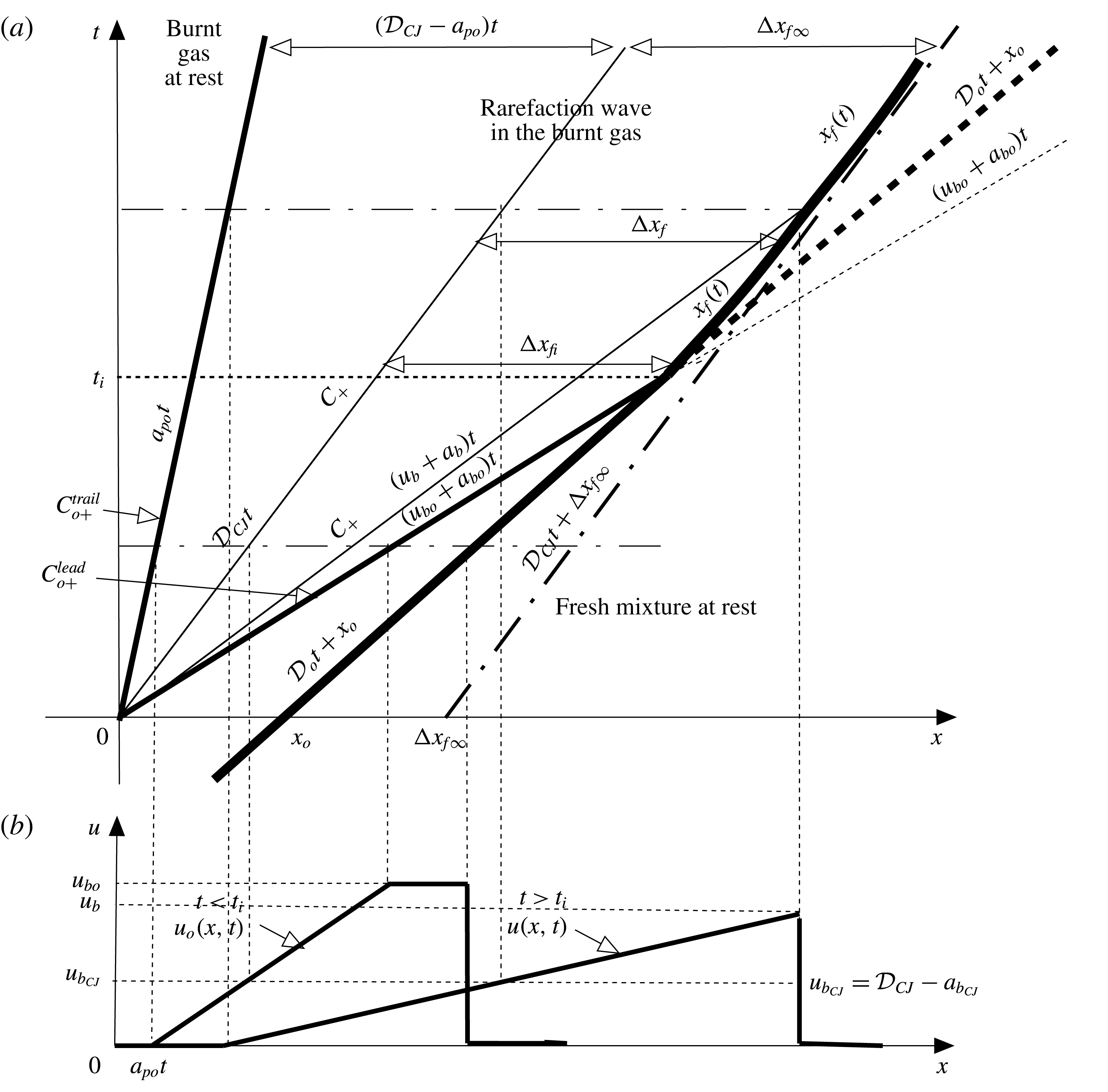
of the centred rarefaction wave. Notice the particular characteristic
 $x={\mathcal{D}}_{CJ}t$
. The big thick line corresponds to the trajectory
 $x=x_{f}(t)$
of the detonation considered as a discontinuity and the two other thick lines correspond to the trailing edge and leading edge of the initial centred rarefaction wave. The origin of time is the time at which the piston is suddenly arrested and
 $x_{o}$
denotes the position of the detonation at this moment. The time at which the leading edge of the rarefaction wave overtakes the detonation is denoted
 $t_{i}$
. The size of the rarefaction wave just prior the interaction with the detonation front is
 $L_{i}=(u_{bo}+a_{bo}-a_{po})t_{i}=[(\unicode[STIX]{x1D6FE}+1)/2]u_{bo}t_{i}$
. (b) Instantaneous profiles of the flow velocity in the burnt gas.

The problem addressed here is the relaxation toward the CJ regime when the piston is suddenly arrested, so that a rarefaction wave starts to develop in the burnt gas. The effect upon the detonation wave is delayed by the time lag
 $t_{i}$
necessary for the leading edge of the rarefaction wave to overtake the detonation. This delay is well defined thanks to the separation of length scales between the flow in the burnt gas and the detonation thickness
 $l_{deto}$
,
 $d\gg l_{deto}$
. If the deceleration of the piston (from the constant velocity
 $v_{p}$
to zero) takes place in an infinitely small time interval (i.e. instantaneously) the rarefaction wave takes initially the self-similar form of the isentropic solution of the Euler equations, called a centred rarefaction wave, see the text book of Courant & Friedrichs (Reference Courant and Friedrichs1948) and § A.2. The flow velocity increases linearly in space across the rarefaction wave from zero (piston at rest) to
 $v_{p}$
, and depends on space
 $x$
and time
 $t$
through
 $x/t$
, see figure 1. The thickness of the centred rarefaction wave increasing linearly with the time, its leading edge catches the tail of the detonation structure at finite time,
 $t=t_{i}$
. This is because the velocity of the leading edge of the centred wave is sonic relatively to the gas flow while the flow of burnt gas behind the overdriven detonation is subsonic relatively to the lead shock. The velocity of the lead shock starts to decrease at
 $t=t_{i}$
so that the flow of burnt gas is no longer isentropic at
 $t>t_{i}$
and the rarefaction wave is no longer self-similar. Hopefully the variation of entropy can be neglected close to the CJ regime which is a marginal solution in the parameters space of ‘pressure-specific volume’.
2.1 Constitutive equations
Introducing the differential operator
 $$\begin{eqnarray}\displaystyle \frac{\text{D}}{\text{D}t}\equiv \frac{\unicode[STIX]{x2202}}{\unicode[STIX]{x2202}t}+u\frac{\unicode[STIX]{x2202}}{\unicode[STIX]{x2202}x}, & & \displaystyle\end{eqnarray}$$
and neglecting the viscosity and the conductivity, the equations governing the one-dimensional flow of a reacting gaseous mixture, considered as an ideal gas
 $p/\unicode[STIX]{x1D70C}=(c_{p}-c_{v})T$
with constant specific heats per unit of mass
 $c_{p}$
and
 $c_{v}$
,
 $\unicode[STIX]{x1D6FE}\equiv c_{p}/c_{v}=\text{cst.}$
, take the form
 $$\begin{eqnarray}\displaystyle \frac{1}{\unicode[STIX]{x1D70C}}\frac{\text{D}}{\text{D}t}\unicode[STIX]{x1D70C}+\frac{\unicode[STIX]{x2202}u}{\unicode[STIX]{x2202}x}=0,\quad \frac{\text{D}}{\text{D}t}u=-\frac{1}{\unicode[STIX]{x1D70C}}\frac{\unicode[STIX]{x2202}p}{\unicode[STIX]{x2202}x}, & & \displaystyle\end{eqnarray}$$
 $$\begin{eqnarray}\displaystyle \frac{\text{D}}{\text{D}t}\left[\ln T-\frac{(\unicode[STIX]{x1D6FE}-1)}{\unicode[STIX]{x1D6FE}}\ln p\right]=\frac{q_{m}}{c_{p}T}\frac{{\dot{w}}}{t_{r}},\quad \frac{\text{D}}{\text{D}t}Y=\frac{{\dot{w}}}{t_{r}}, & & \displaystyle\end{eqnarray}$$
where
 $\unicode[STIX]{x1D70C}$
,
 $u$
,
 $p$
,
 $T$
,
 $Y$
,
 $q_{m}$
,
 $t_{r}$
and
 ${\dot{w}}$
are respectively the density, the flow velocity in the laboratory frame, the pressure, the temperature, the progress variable (
 $Y=0$
in the initial mixture and
 $Y=1$
in the burnt gas), the chemical heat release per unit mass of mixture, the reaction time and the non-dimensional reaction rate. The first equation in (2.3) is the equation for the conservation of energy, written in the form of a production of entropy by the rate of heat release. The problem is closed by the chemical kinetics controlling the heat release. In the simplest case of a one-step irreversible reaction sensitive to the temperature, neglecting the pressure effect for simplicity, the reaction rate
 ${\dot{w}}$
is a function of
 $Y$
and
 $T$
,
 ${\dot{w}}(Y,T)>0$
, where
 $1-Y$
is the reduced mass fraction of the reactive species. At the initial temperature
 $T_{u}$
the system is frozen,
 ${\dot{w}}(Y,T_{u})=0$
, in a composition
 $Y=0$
, far from the chemical equilibrium in the burnt gas,
 $Y=1,T=T_{b}$
,
 ${\dot{w}}(1,T_{b})=0$
. The formulation is easily extended to a multiple-step chemical scheme.
Introducing the sound speed
 $a=\sqrt{\unicode[STIX]{x1D6FE}p/\unicode[STIX]{x1D70C}}$
and eliminating the temperature in the left-hand side of (2.3) using
 $(c_{p}-c_{v})T=p/\unicode[STIX]{x1D70C}$
, the density can be eliminated from the Euler equations (2.2) to take the form of two nonlinear hyperbolic equations for
 $p$
and
 $u$
, extending the Riemann characteristic equations to reacting mixtures,
 $$\begin{eqnarray}\displaystyle \frac{1}{\unicode[STIX]{x1D6FE}}\frac{\text{D}^{\pm }}{\text{D}t}\ln p\pm \frac{1}{a}\frac{\text{D}^{\pm }}{\text{D}t}u=\frac{q_{m}}{c_{p}T}\frac{{\dot{w}}(Y,T)}{t_{r}}, & & \displaystyle\end{eqnarray}$$
where the two following differential operators have been introduced
 $$\begin{eqnarray}\displaystyle \frac{\text{D}^{\pm }}{\text{D}t}\equiv \frac{\unicode[STIX]{x2202}}{\unicode[STIX]{x2202}t}+(u\pm a)\frac{\unicode[STIX]{x2202}}{\unicode[STIX]{x2202}x}, & & \displaystyle\end{eqnarray}$$
see Clavin & Searby (Reference Clavin and Searby2016). In an inert gas (
 ${\dot{w}}=0$
) the linearized version of (2.4) reduces to acoustic waves propagating in two opposite directions.
2.2 Boundary conditions and multiple scale analysis
Because of the difference of time scales between the elastic collisions and the inelastic collisions that are responsible for the chemical heat release, a detonation wave is constituted of an inert shock front followed by a reaction zone (Zeldovich–von Neumann–Döring (ZND) structure). Considering the lead shock as a discontinuity in the flow of inert gas, the conditions in the compressed gas at the shock front, called the Neumann state and denoted by
 $N$
, take the form
 $$\begin{eqnarray}\displaystyle \frac{p_{N}}{p_{u}}=1+\frac{2\unicode[STIX]{x1D6FE}}{\unicode[STIX]{x1D6FE}+1}(M_{u}^{2}-1),\quad \frac{\unicode[STIX]{x1D70C}_{N}}{\unicode[STIX]{x1D70C}_{u}}=\frac{1+(M_{u}^{2}-1)}{1+\displaystyle \frac{\unicode[STIX]{x1D6FE}-1}{\unicode[STIX]{x1D6FE}+1}(M_{u}^{2}-1)},\quad \frac{u_{N}}{a_{u}}=\left(1-\frac{\unicode[STIX]{x1D70C}_{u}}{\unicode[STIX]{x1D70C}_{N}}\right)M_{u}, & & \displaystyle \nonumber\\ \displaystyle & & \displaystyle\end{eqnarray}$$
where the subscript
 $u$
denotes the fresh mixture at rest,
 $M_{u}(t)\equiv {\mathcal{D}}/a_{u}$
. These well-known Rankine–Hugoniot conditions are obtained by the conservation of mass,
 $\unicode[STIX]{x1D70C}_{N}({\mathcal{D}}-u_{N})=\unicode[STIX]{x1D70C}_{u}{\mathcal{D}}$
, momentum and total energy across the discontinuity. The propagation is supersonic,
 $M_{u}>1$
, with an increase of entropy,
 $s_{N}>s_{u}$
, imposed by the dissipative mechanisms inside the inner structure of the shock, see text books.
In addition to the boundary conditions at the Neumann state (2.6),
 $Y=0$
,
 ${\dot{w}}(0,T_{N})\neq 0$
,
 $p=p_{N},\unicode[STIX]{x1D70C}=\unicode[STIX]{x1D70C}_{N}$
and
 $u=u_{N}$
, a boundary condition is required in the burnt gas for solving the detonation dynamics. Generally the latter condition corresponds to the state of the burnt gas at rest nearby the piston. The problem simplifies when the length scale
 $l_{ext}$
of the flow in the burnt gas (approximately the thickness of the rarefaction wave) is larger than the detonation thickness
 $l_{deto}\approx a_{N}t_{r}$
,
 $l_{ext}\gg l_{deto}$
, so that the problem is addressed by a multiple scale analysis. The solution can be decomposed into two regions, a thin zone for the internal structure of the detonation wave (
 ${\dot{w}}\neq 0$
) and a large zone for the external flow
 $u_{ext}(x,t)$
of the rarefaction wave in the burnt gas (
 ${\dot{w}}=0$
). The problem is then solved by matching the inner solution with the external flow. Introducing the equation for the trajectory of the shock front
 $x=x_{f}(t)$
, the study of the inner structure of the detonation is performed using a non-dimensional coordinate of order unity
 $\unicode[STIX]{x1D709}=(x-x_{f}(t))/l_{deto}$
. For a detonation propagating from left to right,
 ${\dot{x}}_{f}\equiv \text{d}x_{f}/\text{d}t>0$
,
 $u\geqslant 0$
, as in figure 1, the initial mixture and the compressed gas correspond respectively to
 $\unicode[STIX]{x1D709}>0$
and
 $\unicode[STIX]{x1D709}<0$
. The matching region corresponds to
 $-l_{ext}\ll x-x_{f}(t)\ll -l_{deto}$
. In terms of the inner variable
 $\unicode[STIX]{x1D709}$
, the boundary condition in the burnt gas to be used in the analysis of the inner structure corresponds to
 $$\begin{eqnarray}\displaystyle \unicode[STIX]{x1D709}\rightarrow -\infty :\quad u=u_{b} & & \displaystyle\end{eqnarray}$$
where
 $u_{b}$
is determined by the matching condition with the external flow
 $u_{ext}(x_{f}(t)+l_{deto}\unicode[STIX]{x1D709},t)$
. To leading order in the limit
 $l_{ext}\gg l_{deto}$
, the variations of the external flow for variations of
 $\unicode[STIX]{x1D709}$
of order unity are negligible,
 $$\begin{eqnarray}\displaystyle u_{b}(t)\approx u_{ext}(x_{f}(t),t). & & \displaystyle\end{eqnarray}$$
Notice that
 $u_{b}(t)$
is an outcome of the analysis even when the external flow field
 $u_{ext}(x_{,}t)$
is prescribed. To the leading order of the multiple length scale analysis,
 $l_{ext}/l_{deto}\gg 1$
, the instantaneous velocity of the lead shock
 ${\mathcal{D}}(t)=\text{d}x_{f}/\text{d}t$
is obtained by the inner solution of (2.2)–(2.3) with the boundary conditions (2.6) at
 $\unicode[STIX]{x1D709}=0$
(Neumann state) and (2.7)–(2.8) at
 $\unicode[STIX]{x1D709}\rightarrow -\infty$
(burnt gas).
3 Decay of discontinuous detonation fronts
Before taking the unsteady inner structure into account, it is worth extending the pioneering analysis of Levin & Chernyi (Reference Levin and Chernyi1967) for
 $M_{u}\gg 1$
(detonation structure in steady state) to the case of small heat release
 $M_{u}-1\ll 1$
, which is the approximation used in § 4. If the piston is brought to an instantaneous halt, the analysis of the detonation decay is drastically simplified when the burnt gas can be approximately described by a centred rarefaction wave during the whole decay. Thanks to the marginal character of the CJ regime, this approximation is valid when the propagation Mach number is sufficiently close to
 $M_{u_{CJ}}$
as recalled now.
3.1 Quasi-isentropic condition in the burnt gas
Consider an overdriven detonation close to the CJ regime, characterized by the small parameter
 $\unicode[STIX]{x1D700}$
 $$\begin{eqnarray}\displaystyle \unicode[STIX]{x1D700}\equiv \frac{(M_{u}^{2}-M_{u_{CJ}}^{2})}{(M_{u_{CJ}}^{2}-1)}\ll 1. & & \displaystyle\end{eqnarray}$$
The pressure and the density in the burnt gas, expressed in terms of the propagation Mach number
 $M_{u}$
, can be written in the form of an expansion in powers of
 $\unicode[STIX]{x1D700}^{1/2}$
, see § A.1. Introducing the notations
 $$\begin{eqnarray}\displaystyle A_{1}\equiv \frac{\unicode[STIX]{x1D6FE}(M_{u_{CJ}}^{2}-1)}{1+\unicode[STIX]{x1D6FE}M_{u_{CJ}}^{2}},\quad \text{and}\quad A_{2}\equiv \sqrt{\frac{M_{u_{CJ}}^{2}+1}{M_{u_{CJ}}^{2}}}, & & \displaystyle\end{eqnarray}$$
equation (A 7) leads to the departure of
 $p_{b}$
and
 $\unicode[STIX]{x1D708}_{b}\equiv 1/\unicode[STIX]{x1D70C}_{b}$
from their CJ values in the form
 $$\begin{eqnarray}\displaystyle & \displaystyle \frac{(p_{b}-p_{b_{CJ}})}{p_{b_{CJ}}}=A_{1}[A_{2}\sqrt{\unicode[STIX]{x1D700}}+\unicode[STIX]{x1D700}]+O(\unicode[STIX]{x1D700}^{3/2}), & \displaystyle\end{eqnarray}$$
 $$\begin{eqnarray}\displaystyle & \displaystyle \unicode[STIX]{x1D6FE}\frac{(\unicode[STIX]{x1D708}_{b}-\unicode[STIX]{x1D708}_{b_{CJ}})}{\unicode[STIX]{x1D708}_{b_{CJ}}}=-\left[\frac{(p_{b}-p_{b_{CJ}})}{p_{b_{CJ}}}-A_{1}\frac{(M_{u}^{2}-M_{u_{CJ}}^{2})}{M_{u_{CJ}}^{2}}\right]\frac{M_{u_{CJ}}^{2}}{M_{u}^{2}}, & \displaystyle\end{eqnarray}$$
where the second term in the bracket on the right-hand side of (3.4) is of order
 $\unicode[STIX]{x1D700}$
. According to the thermodynamic relation
 $\unicode[STIX]{x1D6FF}s/c_{v}=\unicode[STIX]{x1D6FF}p/p+\unicode[STIX]{x1D6FE}\unicode[STIX]{x1D6FF}\unicode[STIX]{x1D708}/\unicode[STIX]{x1D708}$
, equations (3.3)–(3.4) show that the isentropic condition is verified at the leading order in the limit
 $\unicode[STIX]{x1D700}\ll 1$
,
 $\unicode[STIX]{x1D6FF}s/c_{v}\ll \unicode[STIX]{x1D6FF}p/p$
,
 $$\begin{eqnarray}\displaystyle \unicode[STIX]{x1D700}\ll 1:\quad \unicode[STIX]{x1D6FF}p_{b}/p_{b_{CJ}}=O(\sqrt{\unicode[STIX]{x1D700}}),\quad \unicode[STIX]{x1D6FF}s_{b}/c_{v}=(\unicode[STIX]{x1D6FF}p_{b}/p_{b_{CJ}})+\unicode[STIX]{x1D6FE}(\unicode[STIX]{x1D6FF}\unicode[STIX]{x1D708}_{b}/\unicode[STIX]{x1D708}_{b_{CJ}})=O(\unicode[STIX]{x1D700}), & & \displaystyle\end{eqnarray}$$
where
 $\unicode[STIX]{x1D6FF}p_{b}=p_{b}-p_{b_{CJ}}$
and
 $\unicode[STIX]{x1D6FF}\unicode[STIX]{x1D708}_{b}=\unicode[STIX]{x1D708}_{b}-\unicode[STIX]{x1D708}_{b_{CJ}}$
.
The condition in (3.1) for a quasi-isentropic approximation,
 $(M_{u}^{2}-M_{u_{CJ}}^{2})\ll (M_{u_{CJ}}^{2}-1)$
, includes the limit of small heat release
 $(M_{u_{CJ}}-1)\ll 1$
which is used in § 4,
 $$\begin{eqnarray}\displaystyle (M_{u}^{2}-M_{u_{CJ}}^{2})\ll (M_{u_{CJ}}^{2}-1)\ll 1. & & \displaystyle\end{eqnarray}$$
3.2 The rarefaction wave behind a slightly overdriven detonation
Consider a slightly overdriven detonation propagating initially with a constant velocity
 ${\mathcal{D}}_{o}>{\mathcal{D}}_{CJ}$
satisfying the condition
 $\unicode[STIX]{x1D700}\ll 1$
. From now on,
 $\unicode[STIX]{x1D700}$
is defined by (3.1) when
 $M_{u}$
is replaced by the initial propagation Mach number
 ${\mathcal{D}}_{o}/a_{u}$
,
 $$\begin{eqnarray}\displaystyle \unicode[STIX]{x1D700}\equiv ({\mathcal{D}}_{o}^{2}-{\mathcal{D}}_{CJ}^{2})/({\mathcal{D}}_{CJ}^{2}-a_{u}^{2})\ll 1. & & \displaystyle\end{eqnarray}$$
When the velocity of the detonation front
 ${\mathcal{D}}(t)$
is decreasing,
 ${\mathcal{D}}_{u_{CJ}}\leqslant {\mathcal{D}}<{\mathcal{D}}_{o}$
the quantity
 $({\mathcal{D}}^{2}-{\mathcal{D}}_{CJ}^{2})/({\mathcal{D}}_{CJ}^{2}-a_{u}^{2})$
is smaller than
 $\unicode[STIX]{x1D700}$
but of the same order as
 $\unicode[STIX]{x1D700}$
. According to (A 12)–(A 14), the flow
 $u_{o}(x,t)$
in the centred rarefaction wave, generated in the burnt gas as soon as the piston is suddenly stopped at
 $t=0$
, takes the form of a self-similar solution of the isentropic Euler equations recalled in § A.2, see also figure 1,
 $$\begin{eqnarray}\displaystyle 0<t<t_{i}:\quad 0\leqslant x\leqslant a_{po}t:\,u_{o}=0,\quad (u_{bo}+a_{bo})t<x<{\mathcal{D}}_{o}t+x_{o}:\,u_{o}=u_{bo},\qquad & & \displaystyle\end{eqnarray}$$
 $$\begin{eqnarray}\displaystyle a_{po}t\leqslant x\leqslant (u_{bo}+a_{bo})t:\quad u_{o}(x,t)=\frac{2}{(\unicode[STIX]{x1D6FE}+1)}\left[\frac{x}{t}-a_{po}\right], & & \displaystyle\end{eqnarray}$$
where
 $u_{bo}$
and
 $a_{bo}$
are respectively the flow velocity and the sound speed in the burnt gas adjacent to the detonation front propagating with the constant velocity
 ${\mathcal{D}}_{o}$
and
 $a_{po}=a_{bo}-(\unicode[STIX]{x1D6FE}-1)u_{bo}/2$
is the sound speed in the quiescent gas adjacent to the piston at rest. The subscript
 $o$
means that this flow is associated with the period for which the detonation still propagates with its initial constant velocity
 ${\mathcal{D}}_{o}$
, the instantaneous position of the detonation front
 $x_{f}(t)$
being
 $t<t_{i}:\,x_{f}={\mathcal{D}}_{o}t+x_{o}$
where
 $x_{o}$
denotes the position of the detonation at
 $t=0$
i.e. when the piston is suddenly stopped, see figure 1. The flow behind the detonation,
 $x\leqslant x_{f}(t)$
, is usually no longer given by (3.9) as soon as the leading edge of the rarefaction wave interacts with the detonation front, i.e. for
 $t>t_{i}$
. Generally, during the decrease of the detonation velocity
 $\text{d}x_{f}/\text{d}t\equiv {\mathcal{D}}(t)$
from
 ${\mathcal{D}}_{o}$
down to
 ${\mathcal{D}}_{CJ}$
(
 $t>t_{i}:D_{CJ}\leqslant {\mathcal{D}}(t)<{\mathcal{D}}_{o}$
), both the entropy and the Riemann invariant
 $J_{-}\equiv u_{b}-2a_{b}/(\unicode[STIX]{x1D6FE}-1)$
start to vary with
 ${\mathcal{D}}(t)$
. However, when the initial detonation velocity
 ${\mathcal{D}}_{o}$
is close to
 ${\mathcal{D}}_{CJ}$
, these variations are negligible at the leading order in the limit (3.7),
 $\unicode[STIX]{x1D700}\ll 1$
, as shown now. The ideal gas law
 $a_{b}/a_{b_{CJ}}=\sqrt{(p_{b}/p_{b_{CJ}})(\unicode[STIX]{x1D70C}_{b_{CJ}}/\unicode[STIX]{x1D70C}_{b})}$
and the mass conservation
 $\unicode[STIX]{x1D70C}_{b}({\mathcal{D}}-u_{b})=\unicode[STIX]{x1D70C}_{u}{\mathcal{D}}$
yield
 $$\begin{eqnarray}\displaystyle -\frac{2}{\unicode[STIX]{x1D6FE}-1}\frac{\unicode[STIX]{x1D6FF}a_{b}}{a_{b_{CJ}}} & = & \displaystyle -\frac{1}{\unicode[STIX]{x1D6FE}-1}\left[\frac{\unicode[STIX]{x1D6FF}p_{b}}{p_{b_{CJ}}}+\unicode[STIX]{x1D6FF}\left(\frac{\unicode[STIX]{x1D70C}_{b_{CJ}}}{\unicode[STIX]{x1D70C}_{b}}\right)\right],\end{eqnarray}$$
 $$\begin{eqnarray}\displaystyle \frac{\unicode[STIX]{x1D6FF}u_{b}}{a_{b_{CJ}}} & = & \displaystyle -\frac{\unicode[STIX]{x1D70C}_{u}{\mathcal{D}}}{\unicode[STIX]{x1D70C}_{b_{CJ}}a_{b_{CJ}}}\unicode[STIX]{x1D6FF}\left(\frac{\unicode[STIX]{x1D70C}_{b_{CJ}}}{\unicode[STIX]{x1D70C}_{b}}\right)+\left(1-\frac{\unicode[STIX]{x1D70C}_{u}}{\unicode[STIX]{x1D70C}_{b}}\right)\frac{{\mathcal{D}}_{CJ}}{a_{b_{CJ}}}\frac{\unicode[STIX]{x1D6FF}{\mathcal{D}}}{{\mathcal{D}}_{CJ}}.\end{eqnarray}$$
Using the sonic condition of the CJ wave,
 ${\mathcal{D}}_{CJ}-u_{b_{CJ}}=a_{b_{CJ}}$
,
 $\unicode[STIX]{x1D70C}_{b_{CJ}}a_{b_{CJ}}=\unicode[STIX]{x1D70C}_{u}D_{CJ}$
and neglecting terms of order smaller than
 $\unicode[STIX]{x1D700}$
, equation (3.11) yields
 $$\begin{eqnarray}\displaystyle \frac{\unicode[STIX]{x1D6FF}u_{b}}{a_{b_{CJ}}}=-\unicode[STIX]{x1D6FF}\left(\frac{\unicode[STIX]{x1D70C}_{b_{CJ}}}{\unicode[STIX]{x1D70C}_{b}}\right)+\frac{\unicode[STIX]{x1D6FF}{\mathcal{D}}}{{\mathcal{D}}_{CJ}}. & & \displaystyle\end{eqnarray}$$
Adding (3.10) and (3.12) then shows
 $$\begin{eqnarray}\displaystyle \frac{\unicode[STIX]{x1D6FF}J_{-}}{a_{b_{CJ}}}=-\frac{1}{\unicode[STIX]{x1D6FE}-1}\frac{\unicode[STIX]{x1D6FF}s}{c_{v}}+\frac{\unicode[STIX]{x1D6FF}{\mathcal{D}}}{{\mathcal{D}}_{CJ}}+\text{terms smaller than }\unicode[STIX]{x1D700}. & & \displaystyle\end{eqnarray}$$
When the detonation velocity decreases, the order of magnitude of the variation
 $\unicode[STIX]{x1D6FF}J_{-}/a_{b_{CJ}}$
is, according to (3.13), the same as for
 $\unicode[STIX]{x1D6FF}s/c_{v}$
. Then, according to (3.5),
 $\unicode[STIX]{x1D6FF}s/c_{v}=O(\unicode[STIX]{x1D700})$
, the variation of
 $J_{-}$
,
 $\unicode[STIX]{x1D6FF}J_{-}/a_{b_{CJ}}=O(\unicode[STIX]{x1D700})$
, is smaller than the variation of the flow velocity,
 $\unicode[STIX]{x1D6FF}u_{b}/a_{b_{CJ}}=O(\sqrt{\unicode[STIX]{x1D700}})$
, see (3.3), (3.4). The order of magnitude for the sound speed in the quiescent gas adjacent to the piston at rest is, according to (A 9) and (A 14)–(A 16),
 $$\begin{eqnarray}\displaystyle (a_{po}-a_{p_{CJ}})/a_{b_{CJ}}=O(\unicode[STIX]{x1D700}). & & \displaystyle\end{eqnarray}$$
Neglecting terms of order
 $\unicode[STIX]{x1D700}$
, the situation is somehow similar to the case of weak shocks described by Friedrichs (Reference Friedrichs1948); the flow behind the detonation has a constant entropy and a constant Riemann invariant
 $J_{-}$
. For such flows the
 $C_{+}$
characteristics (along which the Riemann invariant
 $J_{+}$
is constant) are straight lines, see Courant & Friedrichs (Reference Courant and Friedrichs1948) and § A.2. Therefore, the rarefaction wave for
 $t>t_{i}$
is just the continuation of that for
 $t<t_{i}$
. In other words, restricting attention to the leading order in the limit
 $\unicode[STIX]{x1D700}\rightarrow 0$
, the decelerating detonation does not influence the burnt gas flow, which continues to be part of the centred rarefaction for
 $t<t_{i}$
when the detonation is moving at the constant velocity
 ${\mathcal{D}}_{o}$
, see figure 1.
3.3 Sonic condition during the decay
When the modification to the centred rarefaction wave is neglected, the trajectory of the detonation front
 $x_{f}(t)$
is simply determined by requiring that the flow velocity (3.9) at
 $x=x_{f}(t)$
satisfies the jump conditions across a detonation (hydrodynamic discontinuity) propagating at the velocity
 ${\mathcal{D}}=\text{d}x_{f}/\text{d}t$
,
 $u_{o}(x_{f},t)=u_{b}(t)$
,
 $$\begin{eqnarray}\displaystyle u_{b}(t)=\frac{2}{(\unicode[STIX]{x1D6FE}+1)}\left[\frac{x_{f}}{t}-a_{po}\right]. & & \displaystyle\end{eqnarray}$$
Subtracting the first equation in (A 16) from (3.15) and neglecting terms of order
 $\unicode[STIX]{x1D700}$
yields
 $$\begin{eqnarray}\displaystyle u_{b}-u_{b_{CJ}}=\frac{2}{\unicode[STIX]{x1D6FE}+1}\left[\frac{x_{f}}{t}-{\mathcal{D}}_{CJ}\right], & & \displaystyle\end{eqnarray}$$
where, according to (3.14), the quantity
 $(a_{po}-a_{p_{CJ}})/a_{b_{CJ}}$
has been neglected in front of
 $(u_{b}-u_{b_{CJ}})/a_{b_{CJ}}=O(\sqrt{\unicode[STIX]{x1D700}})$
. The expression of the left-hand side of (3.16) in terms of
 $M_{u}=(\text{d}x_{f}/\text{d}t)/a_{u}$
is obtained from (3.3), (3.4) using mass conservation,
 $u_{b}({\mathcal{D}})=(1-\unicode[STIX]{x1D70C}_{u}/\unicode[STIX]{x1D70C}_{b}){\mathcal{D}}$
. Retaining only the leading-order term in the limit (3.1) yields
 $$\begin{eqnarray}\displaystyle \frac{u_{b}-u_{b_{CJ}}}{a_{u}} & = & \displaystyle \frac{2}{\unicode[STIX]{x1D6FE}+1}\frac{\left(M_{u_{CJ}}^{2}-1\right)}{2M_{u_{CJ}}}A_{2}\sqrt{\unicode[STIX]{x1D700}}+\text{terms of order }\unicode[STIX]{x1D700}\end{eqnarray}$$
 $$\begin{eqnarray}\displaystyle & {\approx} & \displaystyle \frac{2}{\unicode[STIX]{x1D6FE}+1}\frac{1}{A_{3}}\sqrt{\frac{1}{a_{u}}\frac{\text{d}}{\text{d}t}(x_{f}-{\mathcal{D}}_{CJ}t)},\quad \text{where}~A_{3}\equiv \frac{M_{u_{CJ}}^{3/2}}{\sqrt{(M_{u_{CJ}}^{4}-1)/2}}\end{eqnarray}$$
and where the expression
 $M_{u}-M_{u_{CJ}}=a_{u}^{-1}\text{d}(x_{f}-{\mathcal{D}}_{CJ}t)/\text{d}t$
has been used. Putting together (3.16) and (3.18) yields a differential equation for the front position
 $x_{f}(t)$
,
 $$\begin{eqnarray}\displaystyle \sqrt{\frac{1}{a_{u}}\frac{\text{d}(x_{f}-{\mathcal{D}}_{CJ}t)}{\text{d}t}}=A_{3}\frac{(x_{f}-{\mathcal{D}}_{CJ}t)}{a_{u}t}. & & \displaystyle\end{eqnarray}$$
For future consideration it is worth writing this equation in non-dimensional form by introducing a reference time scale
 $t_{ref}$
which is arbitrary at this level
 $$\begin{eqnarray}\displaystyle \sqrt{\frac{\text{d}\unicode[STIX]{x1D6FC}}{\text{d}\unicode[STIX]{x1D70F}}}=\frac{1}{\sqrt{2}}\frac{\unicode[STIX]{x1D6FC}}{\unicode[STIX]{x1D70F}}\quad \text{where}~\unicode[STIX]{x1D70F}\equiv \frac{t}{t_{ref}},\quad \unicode[STIX]{x1D6FC}\equiv 2A_{3}^{2}\frac{(x_{f}-{\mathcal{D}}_{CJ}t)}{a_{u}t_{ref}}>0. & & \displaystyle\end{eqnarray}$$
Using the beginning of the interaction as the initial condition,
 $t=t_{i}:x_{f}={\mathcal{D}}_{o}t_{i}+x_{o}$
(see figure 1), written in non-dimensional form,
 $\unicode[STIX]{x1D70F}=\unicode[STIX]{x1D70F}_{i}:\unicode[STIX]{x1D6FC}=\unicode[STIX]{x1D6FC}_{i}$
where
 $\unicode[STIX]{x1D6FC}_{i}\equiv 2A_{3}^{2}[({\mathcal{D}}_{o}-{\mathcal{D}}_{CJ})t_{i}+x_{o}]/a_{u}t_{ref}$
, integrating (3.20), yields
 $$\begin{eqnarray}\displaystyle \unicode[STIX]{x1D70F}\geqslant \unicode[STIX]{x1D70F}_{i}:\quad \frac{1}{\unicode[STIX]{x1D6FC}}=\frac{1}{2}\left(\frac{1}{\unicode[STIX]{x1D70F}}-\frac{1}{\unicode[STIX]{x1D70F}_{i}}\right)+\frac{1}{\unicode[STIX]{x1D6FC}_{i}}, & & \displaystyle\end{eqnarray}$$
and in the long-time limit
 $$\begin{eqnarray}\displaystyle \lim _{\unicode[STIX]{x1D70F}\rightarrow \infty }\unicode[STIX]{x1D6FC}=\unicode[STIX]{x1D6FC}_{\infty }\quad \text{where}~\frac{1}{\unicode[STIX]{x1D6FC}_{\infty }}\equiv \frac{1}{\unicode[STIX]{x1D6FC}_{i}}-\frac{1}{2\unicode[STIX]{x1D70F}_{i}}. & & \displaystyle\end{eqnarray}$$
According to the definition of
 $\unicode[STIX]{x1D6FC}$
in (3.20), the asymptotic value
 $\unicode[STIX]{x1D6FC}_{\infty }$
can also be expressed in terms of the length
 $\unicode[STIX]{x0394}x_{f\infty }=\lim _{t\rightarrow \infty }(x_{f}-{\mathcal{D}}_{CJ}t)$
in figure 1,
 $\unicode[STIX]{x1D6FC}_{\infty }=2A_{3}^{2}\unicode[STIX]{x0394}x_{f\infty }/(a_{u}t_{ref})$
. The initial condition
 $\unicode[STIX]{x1D6FC}_{i}$
can be expressed in terms of the initial distance from the detonation and the sonic point
 $\unicode[STIX]{x0394}x_{fi}\equiv ({\mathcal{D}}_{o}-{\mathcal{D}}_{CJ})t_{i}+x_{o}$
,
 $\unicode[STIX]{x1D6FC}_{i}=2A_{3}^{2}\unicode[STIX]{x0394}x_{fi}/a_{u}t_{ref}$
so that
 $\unicode[STIX]{x0394}x_{f\infty }$
and
 $\unicode[STIX]{x0394}x_{fi}$
are linked by the relation
 $$\begin{eqnarray}\displaystyle \frac{1}{\unicode[STIX]{x0394}x_{f\infty }}\equiv \frac{1}{\unicode[STIX]{x0394}x_{fi}}-\frac{A_{3}^{2}}{a_{u}t_{i}}. & & \displaystyle\end{eqnarray}$$
According to (3.21), the asymptotic behaviour in the long-time limit takes the form
 $$\begin{eqnarray}\displaystyle & \displaystyle \lim _{\unicode[STIX]{x1D70F}\rightarrow \infty }(\unicode[STIX]{x1D6FC}-\unicode[STIX]{x1D6FC}_{\infty })\approx -\unicode[STIX]{x1D6FC}_{\infty }^{2}/(2\unicode[STIX]{x1D70F}), & \displaystyle\end{eqnarray}$$
 $$\begin{eqnarray}\displaystyle & \displaystyle t\gg t_{i}:\quad 2A_{3}^{2}\frac{x_{f}-{\mathcal{D}}_{CJ}t}{a_{u}t_{ref}}\approx \unicode[STIX]{x1D6FC}_{\infty }-\frac{\unicode[STIX]{x1D6FC}_{\infty }^{2}}{2}\frac{t_{ref}}{t}~\Rightarrow ~\frac{{\mathcal{D}}-{\mathcal{D}}_{CJ}}{a_{u}}\approx A_{3}^{2}\left(\frac{\unicode[STIX]{x0394}x_{f\infty }}{a_{u}t}\right)^{2}, & \displaystyle\end{eqnarray}$$
showing that the detonation velocity decreases toward the velocity of the self-propagating front like the inverse of the time squared. A similar long-time behaviour was obtained by Levin & Chernyi (Reference Levin and Chernyi1967) and by Liñan et al. (Reference Liñan, Kurdyumov and Sanchez2012) for
 $M_{u}\gg 1$
.
According to (3.21)–(3.25), the distance
 $\unicode[STIX]{x0394}x_{f}$
from the detonation front to the point where the flow velocity is sonic (relatively to the front),
 ${\mathcal{D}}-u=a$
, increases with the time from
 $\unicode[STIX]{x0394}x_{fi}$
to
 $\unicode[STIX]{x0394}x_{f\infty }$
,
 $\unicode[STIX]{x0394}x_{fi}<\unicode[STIX]{x0394}x_{f\infty }$
, see (3.23). The distance
 $\unicode[STIX]{x0394}x_{f}$
thus never becomes shorter than
 $\unicode[STIX]{x0394}x_{fi}$
. In other words, during the decay, the sonic condition
 $a+u={\mathcal{D}}$
is satisfied at a finite distance from the front and the distance
 $\unicode[STIX]{x0394}x_{f}$
never shrinks to zero. The sonic condition
 ${\mathcal{D}}_{CJ}-u_{b_{CJ}}=a_{b_{CJ}}$
is satisfied at the detonation front only in the limit
 $t\rightarrow \infty$
when the slope of the flow velocity in the burnt gas becomes zero, see the self-explanatory figure 1. This result, obtained at the leading order in the limit
 $\unicode[STIX]{x1D700}\rightarrow 0$
and not mentioned before, will be useful in the following.
4 Retarded decay of detonation waves for small heat release
The reaction rate and the sound speed introduce natural time and length scales, the chemical reaction time
 $t_{r}$
at the Neumann state in the compressed gas of the lead shock and the detonation thickness
 $l_{deto}=a_{u}t_{r}$
(
 $a_{N}/a_{u}=O(1)$
in real detonations). According to (2.4) the general formulation of the unsteady inner structure of a detonation takes the form of two hyperbolic equations for the pressure
 $p(x,t)$
and the flow velocity
 $u(x,t)$
while the energy equation (2.3) for the temperature
 $T(x,t)$
describes the entropy wave propagating toward the burnt gas with the flow velocity. These three modes, namely the two nonlinear acoustic waves (propagating in opposite directions) and the entropy wave, are fed by the rate of chemical heat release which is strongly sensitive to temperature. The intrinsic dynamics of a detonation front is governed by the unsteadiness of its inner structure. This inner dynamics results from feedback loops controlling the Neumann temperature. In the reference frame attached to the lead shock, the disturbances of velocity, temperature and pressure, issued from the perturbed leading shock, propagate downstream, toward the reaction zone, by both the entropy wave and the downstream running acoustic wave. The so-induced disturbances of the reaction rate are sent back to the lead shock by the upstream running acoustic wave to close the loop. Because the heat release is distributed in space there is a continuous family of such loops. The problem is too complicated for general analytical solutions to be obtained. Near the CJ condition the dynamics was solved analytically by Clavin & Williams (Reference Clavin and Williams2002) in the limiting case of small heat release per unit mass and in the Newtonian approximation. For the sake of completeness, the 2002 analysis is summarized in § B.1. The decay of the detonations is studied here in this limit.
4.1 Detonation model
The analysis is performed using the distinguished limit,
 $$\begin{eqnarray}\displaystyle \unicode[STIX]{x1D716}^{2}\equiv q_{m}/(c_{p}T_{u})\ll 1,\quad (\unicode[STIX]{x1D6FE}-1)/\unicode[STIX]{x1D716}=h~\Rightarrow ~(M_{u_{CJ}}-1)=\unicode[STIX]{x1D716}+O(\unicode[STIX]{x1D716}^{2}), & & \displaystyle\end{eqnarray}$$
where
 $h$
is of order unity or smaller in the limit
 $\unicode[STIX]{x1D716}\rightarrow 0$
, the ordering of
 $(M_{u_{CJ}}-1)$
being obtained from (A 5). The first relation indicates that the relative variation of temperature is of order
 $\unicode[STIX]{x1D716}^{2}$
so that, assuming a polytropic gas, the relative variation of the sound speed is also of order
 $\unicode[STIX]{x1D716}^{2}$
,
 $a/a_{u}=1+O(\unicode[STIX]{x1D716}^{2})$
. In the limit (4.1) the flow is transonic across the whole detonation structure leading to two main simplifications: firstly the variation of the sound speed can be neglected and secondly the dynamical problem is one of two time scales, as discussed now. The propagation velocity (in the reference frame of the lead shock) of the two downstream running waves (acoustic and entropy) are both of the order of the sound speed which is larger by a factor
 $1/\unicode[STIX]{x1D716}$
than the propagation velocity of the upstream running acoustic wave. Therefore, these waves introduce a time lag of the order of the transit time
 $t_{r}\approx l_{deto}/a_{u}$
which is smaller than the time lag introduced by the upstream running acoustic wave of order
 $t_{r}/\unicode[STIX]{x1D716}$
. At the leading order in the limit (4.1), the effects of the downstream running waves are considered as instantaneous. The time scale of the dynamics of the inner structure is the longest time delay in the loops so that the period of oscillations of weakly unstable detonations is
 $$\begin{eqnarray}\displaystyle t_{ref}=t_{r}/\unicode[STIX]{x1D716}, & & \displaystyle\end{eqnarray}$$
see the discussion below (B 4)–(B 6) in § B.1 for more details. For stable detonations the time
 $t_{ref}$
is the typical delay involved by the linear response of the inner structure to small external disturbances as the unsteady rarefaction wave in the burnt gas of an overdriven detonation.
Then it is convenient to introduce the following reduced coordinates of order unity; the non-dimensional time
 $\unicode[STIX]{x1D70F}$
reduced by
 $t_{ref}$
and the non-dimensional distance from the lead shock
 $\unicode[STIX]{x1D709}$
reduced by
 $a_{u}t_{r}$
 $$\begin{eqnarray}\displaystyle \unicode[STIX]{x1D70F}\equiv \frac{t}{t_{ref}}=\unicode[STIX]{x1D716}\frac{t}{t_{r}},\quad \unicode[STIX]{x1D709}\equiv \frac{x-x_{f}(t)}{a_{u}t_{r}},\quad \frac{\unicode[STIX]{x2202}}{\unicode[STIX]{x2202}t}=\frac{1}{t_{r}}\left(\unicode[STIX]{x1D716}\frac{\unicode[STIX]{x2202}}{\unicode[STIX]{x2202}\unicode[STIX]{x1D70F}}-\frac{1}{a_{u}}\frac{\text{d}x_{f}}{\text{d}t}\frac{\unicode[STIX]{x2202}}{\unicode[STIX]{x2202}\unicode[STIX]{x1D709}}\right),\quad \frac{\unicode[STIX]{x2202}}{\unicode[STIX]{x2202}x}=\frac{1}{a_{u}t_{r}}\frac{\unicode[STIX]{x2202}}{\unicode[STIX]{x2202}\unicode[STIX]{x1D709}}, & & \displaystyle \nonumber\\ \displaystyle & & \displaystyle\end{eqnarray}$$
where the
 $x$
-coordinate is orientated as in figure 1, corresponding to
 $\unicode[STIX]{x1D709}<0$
in the shocked gas and
 $\text{d}x_{f}/\text{d}t={\mathcal{D}}(t)>0$
. To avoid confusion, notice that this orientation of the
 $x$
-coordinate, which was used in the pioneering works of Courant & Friedrichs (Reference Courant and Friedrichs1948) and Levin & Chernyi (Reference Levin and Chernyi1967), is the opposite to the one in Clavin & Williams (Reference Clavin and Williams2002) and Clavin & Williams (Reference Clavin and Williams2009). It is also convenient to introduce reduced unknowns; the non-dimensional distance of the lead shock from the sonic point
 $\unicode[STIX]{x1D6FC}(\unicode[STIX]{x1D70F})$
, the non-dimensional difference of velocity between the lead shock and the CJ velocity
 $\dot{\unicode[STIX]{x1D6FC}}_{\unicode[STIX]{x1D70F}}(\unicode[STIX]{x1D70F})\equiv \text{d}\unicode[STIX]{x1D6FC}/\text{d}\unicode[STIX]{x1D70F}>0$
and the non-dimensional flow velocity shifted by the constant term
 $({\mathcal{D}}_{CJ}-a_{u})>0$
,
 $\unicode[STIX]{x1D707}(\unicode[STIX]{x1D709},\unicode[STIX]{x1D70F})$
,
 $$\begin{eqnarray}\displaystyle \unicode[STIX]{x1D6FC}\equiv \frac{x_{f}(t)-{\mathcal{D}}_{CJ}t}{a_{u}t_{r}}>0,\quad \dot{\unicode[STIX]{x1D6FC}}_{\unicode[STIX]{x1D70F}}\equiv \frac{\displaystyle \frac{\text{d}x_{f}}{\text{d}t}-{\mathcal{D}}_{CJ}}{\unicode[STIX]{x1D716}a_{u}},\quad \unicode[STIX]{x1D707}\equiv \frac{1}{\unicode[STIX]{x1D716}a_{u}}[u-({\mathcal{D}}_{CJ}-a_{u})]>0. & & \displaystyle\end{eqnarray}$$
The definition of
 $\unicode[STIX]{x1D6FC}$
in (4.4) is the same as in (3.20),
 $2A_{3}^{2}\approx 1/\unicode[STIX]{x1D716}$
in the limit (4.1).
Introducing the instantaneous distribution of reaction rate
 $w(\unicode[STIX]{x1D709},\dot{\unicode[STIX]{x1D6FC}}_{\unicode[STIX]{x1D70F}})={\dot{w}}(Y,T)$
, Clavin & Williams (Reference Clavin and Williams2002) showed that, to leading order in the limit (4.1), the intrinsic dynamics of the inner structure is reduced to solving a single partial differential equation for the non-dimensional flow velocity
 $\unicode[STIX]{x1D707}(\unicode[STIX]{x1D709},\unicode[STIX]{x1D70F})$
, see § B.1,
 $$\begin{eqnarray}\displaystyle \frac{\unicode[STIX]{x2202}\unicode[STIX]{x1D707}}{\unicode[STIX]{x2202}\unicode[STIX]{x1D70F}}+(\unicode[STIX]{x1D707}-\dot{\unicode[STIX]{x1D6FC}}_{\unicode[STIX]{x1D70F}})\frac{\unicode[STIX]{x2202}\unicode[STIX]{x1D707}}{\unicode[STIX]{x2202}\unicode[STIX]{x1D709}}=\frac{1}{2}w(\unicode[STIX]{x1D709},\dot{\unicode[STIX]{x1D6FC}}_{\unicode[STIX]{x1D70F}}). & & \displaystyle\end{eqnarray}$$
The usual nonlinear term of the Burgers type characterizes transonic flows as in Bdzil & Stewart (Reference Bdzil and Stewart1986). The unknown velocity of the lead shock
 $\dot{\unicode[STIX]{x1D6FC}}_{\unicode[STIX]{x1D70F}}(\unicode[STIX]{x1D70F})$
is obtained by using the boundary conditions (2.6) at the lead shock in (B 3) and (2.7), (2.8) in the burnt gas,
 $$\begin{eqnarray}\displaystyle \unicode[STIX]{x1D709}=0:\,\unicode[STIX]{x1D707}=1+2\,\dot{\unicode[STIX]{x1D6FC}}_{\unicode[STIX]{x1D70F}}(\unicode[STIX]{x1D70F}),\quad \unicode[STIX]{x1D709}\rightarrow -\infty :\,\unicode[STIX]{x1D707}=\unicode[STIX]{x1D707}_{b}. & & \displaystyle\end{eqnarray}$$
Here only the first-order correction to
 $\unicode[STIX]{x1D707}$
is retained at the Neumann state (
 $\unicode[STIX]{x1D709}=0$
), anticipating that
 $\dot{\unicode[STIX]{x1D6FC}}_{\unicode[STIX]{x1D70F}}$
is a small quantity when the propagation regime is sufficiently close to the CJ regime, see (4.14). The pulsations of the detonation are controlled by the thermal sensitivity of the rate of the chemical heat release. The instantaneous distribution of the rate of heat release
 $w(\unicode[STIX]{x1D709},\dot{\unicode[STIX]{x1D6FC}}_{\unicode[STIX]{x1D70F}})$
, to be introduced into the right-hand side of (4.5), is obtained in § B.1 by the solution of (2.3) with the boundary conditions (2.6) at
 $\unicode[STIX]{x1D709}=0$
when the compressional heating is negligible. In the following we will use the approximate expression in (B 13), obtained by a scaling law,
 $$\begin{eqnarray}\displaystyle w(\unicode[STIX]{x1D709},\dot{\unicode[STIX]{x1D6FC}}_{\unicode[STIX]{x1D70F}})\approx \text{e}^{b\dot{\unicode[STIX]{x1D6FC}}_{\unicode[STIX]{x1D70F}}}\overline{w}_{CJ}(\unicode[STIX]{x1D709}\text{e}^{b\dot{\unicode[STIX]{x1D6FC}}_{\unicode[STIX]{x1D70F}}}), & & \displaystyle\end{eqnarray}$$
where
 $\overline{w}_{CJ}(\unicode[STIX]{x1D709})$
is the distribution of heat release rate in the unperturbed CJ wave (
 $\dot{\unicode[STIX]{x1D6FC}}_{\unicode[STIX]{x1D70F}}=0$
) and, according to (B 12),
 $\text{e}^{-b\dot{\unicode[STIX]{x1D6FC}}_{\unicode[STIX]{x1D70F}}}$
is the non-dimensional induction length, the coefficient
 $b$
measuring the thermal sensitivity. The boundary condition
 $\unicode[STIX]{x1D707}_{b}$
in (4.6) is determined in § 4.5 by matching the inner solution with the external flow in the burnt gas. It is worth looking first to the steady state.
4.2 Steady states
Consider first the steady case of a detonation moving at constant velocity
 $\overline{{\mathcal{D}}}$
,
 $\dot{\unicode[STIX]{x1D6FC}}_{\unicode[STIX]{x1D70F}}=\overline{m}$
where, according to (4.4),
 $\overline{m}$
is a positive constant,
 $$\begin{eqnarray}\displaystyle \dot{\unicode[STIX]{x1D6FC}}_{\unicode[STIX]{x1D70F}}=\overline{m}\equiv \frac{\overline{{\mathcal{D}}}-{\mathcal{D}}_{CJ}}{\unicode[STIX]{x1D716}a_{u}}>0, & & \displaystyle\end{eqnarray}$$
the overbar identifying the steady states. The expression of the flow velocity in the burnt gas
 $\overline{\unicode[STIX]{x1D707}}_{b}$
in terms of the detonation velocity
 $\overline{m}$
is obtained by integrating the steady version of (4.5) (
 $\unicode[STIX]{x2202}\unicode[STIX]{x1D707}/\unicode[STIX]{x2202}\unicode[STIX]{x1D70F}=0$
),
 $\text{d}(\overline{\unicode[STIX]{x1D707}}-\overline{m})^{2}/\text{d}\unicode[STIX]{x1D709}=\overline{w}$
, from the burnt gas at
 $\unicode[STIX]{x1D709}=-\infty$
to the lead shock
 $\unicode[STIX]{x1D709}=0$
, using the normalized condition
 $\int _{-\infty }^{0}\overline{w}(\unicode[STIX]{x1D709},\overline{m})\,\text{d}\unicode[STIX]{x1D709}=1$
, valid to the leading order in the limit
 $\unicode[STIX]{x1D716}\ll 1$
, since
 $\overline{w}(\unicode[STIX]{x1D709},\overline{m})={\dot{w}}(\overline{Y},\overline{T})$
and
 $\text{d}\overline{Y}/\text{d}\unicode[STIX]{x1D709}=-{\dot{w}}(\overline{Y},\overline{T})+O(\unicode[STIX]{x1D716})$
with
 $\overline{Y}|_{\unicode[STIX]{x1D709}=0}=0$
and
 $\overline{Y}|_{\unicode[STIX]{x1D709}=-\infty }=1$
. This yields
 $(\overline{\unicode[STIX]{x1D707}}-\overline{m})_{\unicode[STIX]{x1D709}=0}^{2}-(\overline{\unicode[STIX]{x1D707}}-\overline{m})_{\unicode[STIX]{x1D709}=-\infty }^{2}=1$
. Assuming that the departure from the CJ velocity is sufficiently small
 $\overline{m}\ll 1$
,
 $\unicode[STIX]{x1D709}=0:\,\overline{\unicode[STIX]{x1D707}}=1+2\,\overline{m}$
, the integration across the detonation structure then leads to
 $$\begin{eqnarray}\displaystyle (1+\overline{m})^{2}-(\overline{\unicode[STIX]{x1D707}}_{b}-\overline{m})^{2}=1~\Rightarrow ~\overline{\unicode[STIX]{x1D707}}_{b}=\overline{m}+\sqrt{(1+\overline{m})^{2}-1}, & & \displaystyle\end{eqnarray}$$
where the
 $+$
sign is chosen according to the ZND solution. According to (4.9) the flow velocity in the burnt gas takes the form
 $$\begin{eqnarray}\displaystyle \overline{m}\ll 1~\Rightarrow ~\overline{\unicode[STIX]{x1D707}}_{b}^{2}\approx 2\overline{m},\quad \overline{\unicode[STIX]{x1D707}}_{b}\approx \sqrt{2\overline{m}}, & & \displaystyle\end{eqnarray}$$
which is in agreement with (3.3), (3.4) for small
 $\unicode[STIX]{x1D700}$
. The square root in the expression of
 $\overline{\unicode[STIX]{x1D707}}_{b}$
illustrates the marginal character of the CJ regime.
4.3 Flow velocity in the burnt gas
For the decay of detonation, the unknown function
 $\dot{\unicode[STIX]{x1D6FC}}_{\unicode[STIX]{x1D70F}}(\unicode[STIX]{x1D70F})\geqslant 0$
is obtained from (4.5), (4.6) when the boundary condition in the burnt gas
 $\unicode[STIX]{x1D707}_{b}$
is expressed in terms of
 $\dot{\unicode[STIX]{x1D6FC}}_{\unicode[STIX]{x1D70F}}(\unicode[STIX]{x1D70F})$
by matching the inner solution with the external flow. For an inert gas (
 $w=0$
) there is a particular solution of (4.5) of the form
 $$\begin{eqnarray}\displaystyle w=0:\quad \unicode[STIX]{x1D707}_{ext}(\unicode[STIX]{x1D709},\unicode[STIX]{x1D70F})=\frac{\unicode[STIX]{x1D709}+\unicode[STIX]{x1D6FC}(\unicode[STIX]{x1D70F})}{\unicode[STIX]{x1D70F}}. & & \displaystyle\end{eqnarray}$$
In the limit (4.1), the expression (4.11) is precisely that of the centred rarefaction wave (3.9) in the transonic region where
 $\unicode[STIX]{x1D709}$
is of order unity, as shown by using the approximations
 $a_{po}/a_{u}\approx 1$
and
 $\unicode[STIX]{x1D6FE}\approx 1$
and the definition of
 $\unicode[STIX]{x1D70F}$
in (4.3),
 $$\begin{eqnarray}\displaystyle \frac{u}{a_{u}}+1\approx \frac{(x-x_{f})/(a_{u}t_{r})}{t/t_{r}}+\frac{x_{f}/(a_{u}t_{r})}{t/t_{r}}=\frac{\unicode[STIX]{x1D716}}{\unicode[STIX]{x1D70F}}\left[\unicode[STIX]{x1D709}+\frac{x_{f}-{\mathcal{D}}_{CJ}t}{a_{u}t_{r}}\right]+\frac{{\mathcal{D}}_{CJ}}{a_{u}} & & \displaystyle\end{eqnarray}$$
leading to (4.11) because, according to (4.4), one has
 $u/a+1={\mathcal{D}}_{CJ}/a_{u}+\unicode[STIX]{x1D716}\unicode[STIX]{x1D707}$
.
The external flow in the burnt gas therefore takes the form (4.11) if the entropy emitted at
 $\unicode[STIX]{x1D709}=0$
is constant so that the centred rarefaction wave is not disturbed by the dynamics of the detonation. According to the discussion in § 3, this assumption is verified when the propagation velocity is sufficient close to the CJ velocity,
 $\unicode[STIX]{x1D700}\ll 1$
.
4.4 Double limit
One is thus led to analyse the detonation decay near the CJ regime
 $\unicode[STIX]{x1D700}\ll 1$
, for small heat release
 $\unicode[STIX]{x1D716}\equiv \sqrt{q_{m}/(c_{p}T_{u})}\approx (M_{u_{CJ}}-1)\ll 1$
, see (3.7) and (4.1). The problem is thus investigated in the double limit
 $\unicode[STIX]{x1D700}\rightarrow 0$
and
 $\unicode[STIX]{x1D716}\rightarrow 0$
. Considering an initial overdriven detonation (velocity
 ${\mathcal{D}}_{o}$
) verifying (3.7), the propagation Mach number of the decaying detonation satisfies the ordering
 $$\begin{eqnarray}\displaystyle (M_{u}-M_{u_{CJ}})/(M_{u_{CJ}}-1)=O(\unicode[STIX]{x1D700})~\Rightarrow ~(M_{u}-M_{u_{CJ}})=({\mathcal{D}}-{\mathcal{D}}_{CJ})/a_{u}=O(\unicode[STIX]{x1D700}\unicode[STIX]{x1D716}). & & \displaystyle\end{eqnarray}$$
The regimes under consideration correspond to the double limit (3.6) and, according to (4.4), the reduced velocity of the shock front
 $\dot{\unicode[STIX]{x1D6FC}}_{\unicode[STIX]{x1D70F}}$
is a small quantity of order
 $\unicode[STIX]{x1D700}$
 $$\begin{eqnarray}\displaystyle (M_{u}-M_{u_{CJ}})\ll (M_{u_{CJ}}-1)\ll 1~\Rightarrow ~\dot{\unicode[STIX]{x1D6FC}}_{\unicode[STIX]{x1D70F}}=O(\unicode[STIX]{x1D700}), & & \displaystyle\end{eqnarray}$$
with, according to (4.8)–(4.10),
 $\overline{\unicode[STIX]{x1D707}}_{b}=O(\sqrt{\unicode[STIX]{x1D700}})$
, in agreement with (3.3), (3.4). The terms of order
 $\unicode[STIX]{x1D716}^{2}$
at
 $\unicode[STIX]{x1D709}=0$
being neglected in (4.6), the relation
 $\unicode[STIX]{x1D716}^{2}\ll \unicode[STIX]{x1D716}\unicode[STIX]{x1D700}$
should be used in (4.13) for consistency. Then, the double limit to be considered in the asymptotic analysis is
 $$\begin{eqnarray}\displaystyle \unicode[STIX]{x1D700}\rightarrow 0\quad \text{and}\quad \unicode[STIX]{x1D716}\ll \unicode[STIX]{x1D700}. & & \displaystyle\end{eqnarray}$$
Retaining the terms of order
 $\unicode[STIX]{x1D716}^{2}$
would have introduced more tedious calculations but no new physical insights.
To summarize, the decay of the detonation is obtained in the limit (4.15) by the solution of (4.5) satisfying the boundary conditions (4.6),
 $\unicode[STIX]{x1D707}_{b}$
being given by the matching condition with the external flow in (4.11). Anticipating, on the basis of the results in § 3.3, that
 $\unicode[STIX]{x1D6FC}(\unicode[STIX]{x1D70F})$
goes to a constant when
 $\unicode[STIX]{x1D70F}$
increases, the flow velocity in (4.11) goes to zero when
 $\unicode[STIX]{x1D70F}\rightarrow \infty$
for any value of
 $\unicode[STIX]{x1D709}$
of order unity. The value
 $\unicode[STIX]{x1D707}=0$
corresponds effectively to the sonic condition of CJ waves
 ${\mathcal{D}}_{CJ}-u_{b_{CJ}}=a_{b_{CJ}}$
,
 $\lim _{\unicode[STIX]{x1D716}\rightarrow 0}\unicode[STIX]{x1D707}_{b_{CJ}}=0$
, as shown from the expression of
 $\unicode[STIX]{x1D707}$
in (4.4) when using the relation
 $a_{u}\approx a_{b_{CJ}}$
, valid in the limit (4.15).
4.5 Simplification coming from the initial condition
Matching the inner flow with (4.11) becomes simpler when
 $\unicode[STIX]{x1D6FC}\gg 1$
,
 $x_{f}(t)-{\mathcal{D}}_{CJ}t\gg a_{u}t_{r}$
(
 $\unicode[STIX]{x0394}x_{f}\gg a_{u}t_{r}$
in the notation of figure 1), namely when the distance between the lead shock and the point where the sonic condition holds is larger than the detonation thickness. This is automatically satisfied for typical initial conditions, namely when the initial distance between the detonation and the piston at
 $t=0$
(time at which the piston is suddenly arrested) is larger than the detonation thickness,
 $x_{o}\gg a_{u}t_{r}$
, see figure 1. Under such conditions the term
 $\unicode[STIX]{x1D709}$
(of order unity in the internal structure) is negligible in front of
 $\unicode[STIX]{x1D6FC}$
in (4.11). The external flow close to the detonation is nearly uniform and takes the form
 $\unicode[STIX]{x1D707}_{ext}\approx \unicode[STIX]{x1D6FC}(\unicode[STIX]{x1D70F})/\unicode[STIX]{x1D70F}$
. This approximation is equivalent to neglecting the gradient of the reduced velocity of the flow compared to the inverse of the detonation thickness,
 $\unicode[STIX]{x2202}\unicode[STIX]{x1D707}_{ext}/\unicode[STIX]{x2202}\unicode[STIX]{x1D709}=1/\unicode[STIX]{x1D70F}\ll 1$
. Matching then leads to a boundary condition (4.6) in the burnt gas similar to (2.7), (2.8) with
 $$\begin{eqnarray}\displaystyle \unicode[STIX]{x1D707}_{b}(\unicode[STIX]{x1D70F})=\frac{\unicode[STIX]{x1D6FC}(\unicode[STIX]{x1D70F})}{\unicode[STIX]{x1D70F}}=O(\sqrt{\unicode[STIX]{x1D700}}), & & \displaystyle\end{eqnarray}$$
where the same order of magnitude of the flow velocity in the burnt gas as in the steady state near the CJ regime, has been used,
 $\unicode[STIX]{x1D707}_{b}=O(\sqrt{\unicode[STIX]{x1D700}})$
. This condition is compatible with
 $\unicode[STIX]{x1D6FC}\gg 1$
when considering instants of time sufficiently large,
 $\unicode[STIX]{x1D70F}\gg 1/\sqrt{\unicode[STIX]{x1D700}}$
. This condition is automatically satisfied for
 $t>t_{i}$
if
 $t_{i}\gg t_{r}/(\unicode[STIX]{x1D716}\sqrt{\unicode[STIX]{x1D700}})$
that corresponds to an initial distance
 $x_{o}$
that is large compared to the detonation thickness
 $l_{deto}\approx a_{u}t_{r}$
,
 $$\begin{eqnarray}\displaystyle x_{o}\gg a_{u}t_{r}~\Leftrightarrow ~t_{i}\gg t_{r}/(\unicode[STIX]{x1D716}\sqrt{\unicode[STIX]{x1D700}})\quad \text{i.e.}~\unicode[STIX]{x1D70F}_{i}\gg 1/\sqrt{\unicode[STIX]{x1D700}}~\Rightarrow ~\unicode[STIX]{x1D6FC}\gg 1, & & \displaystyle\end{eqnarray}$$
as shown from the relation
 $x_{o}/(a_{u}t_{i})\approx \unicode[STIX]{x1D716}\sqrt{2\unicode[STIX]{x1D700}}$
, which is obtained from the relation
 $x_{o}=[a_{bo}-({\mathcal{D}}_{o}-u_{bo})]t_{i}$
in figure 1 when using (3.3), (3.4) with (A 4), (A 5) and (3.7), neglecting the terms of order
 $\unicode[STIX]{x1D716}^{2}$
in (4.1),
 $(M_{uo}^{2}-1)\approx \unicode[STIX]{x1D716}(1+\unicode[STIX]{x1D700})$
. To summarize, for ordinary initial conditions,
 $x_{o}\gg a_{u}t_{r}$
, the problem is reduced to solving (4.5) using the boundary conditions (4.6) with (4.16).
The solution for a detonation considered as a hydrodynamic discontinuity in § 3 is recovered by the quasi-steady state approximation, namely when the unsteady term is neglected in (4.5). Integrating (4.5) across the detonation structure, from
 $-\infty$
to 0, using the condition of normalization,
 $\int _{-\infty }^{0}w(\unicode[STIX]{x1D709},\dot{\unicode[STIX]{x1D6FC}}_{\unicode[STIX]{x1D70F}})\,\text{d}\unicode[STIX]{x1D709}=1$
, yields
 $$\begin{eqnarray}\displaystyle {\textstyle \frac{1}{2}}(\unicode[STIX]{x1D707}-\dot{\unicode[STIX]{x1D6FC}}_{\unicode[STIX]{x1D70F}})^{2}|_{\unicode[STIX]{x1D709}=-\infty }^{\unicode[STIX]{x1D709}=0}={\textstyle \frac{1}{2}}~\Rightarrow ~{\textstyle \frac{1}{2}}(\unicode[STIX]{x1D707}^{2}|_{\unicode[STIX]{x1D709}=0}-\unicode[STIX]{x1D707}_{b}^{2})-(\unicode[STIX]{x1D707}|_{\unicode[STIX]{x1D709}=0}-\unicode[STIX]{x1D707}_{b})\dot{\unicode[STIX]{x1D6FC}}_{\unicode[STIX]{x1D70F}}={\textstyle \frac{1}{2}}, & & \displaystyle\end{eqnarray}$$
and equation (3.20) is effectively recovered by the boundary conditions (4.6) (4.16) when the terms smaller than
 $\dot{\unicode[STIX]{x1D6FC}}_{\unicode[STIX]{x1D70F}}=O(\unicode[STIX]{x1D700})$
are neglected,
 $\dot{\unicode[STIX]{x1D6FC}}_{\unicode[STIX]{x1D70F}}\equiv \text{d}\unicode[STIX]{x1D6FC}/\text{d}\unicode[STIX]{x1D70F}=(1/2)(\unicode[STIX]{x1D6FC}/\unicode[STIX]{x1D70F})^{2}$
.
4.6 Instantaneous distribution of the rate of heat release
Another simplification concerns the instantaneous distribution of the heat release rate
 $w(\unicode[STIX]{x1D709},\dot{\unicode[STIX]{x1D6FC}}_{\unicode[STIX]{x1D70F}})$
on the right-hand side of (4.5). Its determination becomes more easy if the compressional heating in the thermal equation (2.3) can be neglected, which is the cases if
 $(\unicode[STIX]{x1D6FE}-1)$
is sufficiently small,
 $h\ll 1$
in (4.1) as will be assumed from now on,
 $$\begin{eqnarray}\displaystyle (\unicode[STIX]{x1D6FE}-1)/\unicode[STIX]{x1D716}\ll 1. & & \displaystyle\end{eqnarray}$$
Following the work of Clavin & He (Reference Clavin and He1996), the analysis, recalled in § B.1, leads to (4.7). According to (4.6) and (4.16),
 $\unicode[STIX]{x1D707}(\unicode[STIX]{x1D709},\unicode[STIX]{x1D70F})$
is of order unity close to the lead shock and of order
 $\sqrt{\unicode[STIX]{x1D700}}$
at the end of the reaction zone. Therefore, according to (4.14), the non-dimensional velocity
 $\dot{\unicode[STIX]{x1D6FC}}_{\unicode[STIX]{x1D70F}}(\unicode[STIX]{x1D70F})=O(\unicode[STIX]{x1D700})$
is smaller than
 $\unicode[STIX]{x1D707}(\unicode[STIX]{x1D709},\unicode[STIX]{x1D70F})$
. For stable detonations against planar disturbances only the linear term in the expansion of the instantaneous reaction rate (4.7) in powers of
 $\unicode[STIX]{x1D6FF}\dot{\unicode[STIX]{x1D6FC}}_{\unicode[STIX]{x1D70F}}(\unicode[STIX]{x1D70F})$
is retained at the leading order in the limit (4.15). The corresponding expression of the variation
 $\unicode[STIX]{x1D6FF}w(\unicode[STIX]{x1D709},\dot{\unicode[STIX]{x1D6FC}}_{\unicode[STIX]{x1D70F}})$
is similar to that in the stability analysis of Clavin & Williams (Reference Clavin and Williams2002). Neglecting the terms smaller than
 $\unicode[STIX]{x1D700}$
, equation (4.5) then takes the form
 $$\begin{eqnarray}\displaystyle \frac{\unicode[STIX]{x2202}\unicode[STIX]{x1D707}}{\unicode[STIX]{x2202}\unicode[STIX]{x1D70F}}+[\unicode[STIX]{x1D707}-\dot{\unicode[STIX]{x1D6FC}}_{\unicode[STIX]{x1D70F}}(\unicode[STIX]{x1D70F})]\frac{\unicode[STIX]{x2202}\unicode[STIX]{x1D707}}{\unicode[STIX]{x2202}\unicode[STIX]{x1D709}}=\frac{1}{2}\overline{\unicode[STIX]{x1D714}}(\unicode[STIX]{x1D709})+\frac{b}{2}\overline{\unicode[STIX]{x1D6FA}}(\unicode[STIX]{x1D709})\unicode[STIX]{x1D6FF}\dot{\unicode[STIX]{x1D6FC}}_{\unicode[STIX]{x1D70F}}(\unicode[STIX]{x1D70F})\quad \text{where}~\overline{\unicode[STIX]{x1D6FA}}(\unicode[STIX]{x1D709})\equiv \frac{\text{d}}{\text{d}\unicode[STIX]{x1D709}}[\unicode[STIX]{x1D709}\overline{\unicode[STIX]{x1D714}}(\unicode[STIX]{x1D709})], & & \displaystyle\end{eqnarray}$$
 $$\begin{eqnarray}\displaystyle \int _{-\infty }^{0}\overline{\unicode[STIX]{x1D6FA}}(\unicode[STIX]{x1D709})\,\text{d}\unicode[STIX]{x1D709}=0,\quad \int _{-\infty }^{0}\overline{\unicode[STIX]{x1D714}}(\unicode[STIX]{x1D709})\,\text{d}\unicode[STIX]{x1D709}=1, & & \displaystyle\end{eqnarray}$$
where the coefficient
 $b$
in front of
 $\overline{\unicode[STIX]{x1D6FA}}(\unicode[STIX]{x1D709})$
in (4.20) is a measure of the sensitivity to the Neumann temperature, see (B 12), (B 13). The function
 $\overline{\unicode[STIX]{x1D714}}(\unicode[STIX]{x1D709})$
is the distribution of heat release rate in the unperturbed overdriven detonation, and
 $\overline{\unicode[STIX]{x1D6FA}}(\unicode[STIX]{x1D709})$
characterizes the deformation of the distribution of the overdriven detonation in steady state when the Neumann temperature is modified from its unperturbed value, see (B 10), (B 11).
An implicit relation between the non-dimensional shock position (relative to the sonic point),
 $\unicode[STIX]{x1D6FC}(\unicode[STIX]{x1D70F})\gg 1$
, and its velocity (relative to that of the CJ wave),
 $\dot{\unicode[STIX]{x1D6FC}}_{\unicode[STIX]{x1D70F}}(\unicode[STIX]{x1D70F})\equiv \text{d}\unicode[STIX]{x1D6FC}/\text{d}\unicode[STIX]{x1D70F}=O(\unicode[STIX]{x1D700})$
, is then obtained during the decay (
 $\unicode[STIX]{x1D70F}\geqslant \unicode[STIX]{x1D70F}_{i}$
,
 $\unicode[STIX]{x1D70F}_{i}\equiv \unicode[STIX]{x1D716}t_{i}/t_{r}\gg 1/\sqrt{\unicode[STIX]{x1D700}}$
) by solving the partial differential equation (4.20) for the flow velocity field
 $\unicode[STIX]{x1D707}(\unicode[STIX]{x1D709},\unicode[STIX]{x1D70F})$
with the two boundary conditions (4.6) using (4.16). When equation (4.20) is fully linearized and when the boundary condition (4.16) is replaced by an unperturbed uniform flow,
 $\unicode[STIX]{x1D709}\rightarrow -\infty :\unicode[STIX]{x1D707}=\overline{\unicode[STIX]{x1D707}}_{b}=$
cst., the stability analysis of Clavin & Williams (Reference Clavin and Williams2002) against planar disturbances is recovered, see § B.2.
4.7 Linear dynamics at the beginning of the decay
The initial condition of the detonation decay is a steady weakly overdriven detonation for small heat release in the limit (4.15). Assume to begin with that this initial detonation is stable. Unstable detonations will be considered in § 4.8. Denoting
 $\unicode[STIX]{x1D6FC}_{i}$
the position of the lead shock at time
 $\unicode[STIX]{x1D70F}_{i}$
when the rarefaction wave catches the unperturbed overdriven detonation, the initial conditions are, according to (4.8)–(4.10),
 $$\begin{eqnarray}\displaystyle \unicode[STIX]{x1D70F}=\unicode[STIX]{x1D70F}_{i}:\quad \unicode[STIX]{x1D6FC}=\unicode[STIX]{x1D6FC}_{i},\quad {\mathcal{D}}={\mathcal{D}}_{o},\quad \text{d}\unicode[STIX]{x1D6FC}/\text{d}\unicode[STIX]{x1D70F}=\unicode[STIX]{x1D700},\quad \unicode[STIX]{x1D6FC}_{i}/\unicode[STIX]{x1D70F}_{i}=\sqrt{2\unicode[STIX]{x1D700}}, & & \displaystyle\end{eqnarray}$$
where the last relation comes from (4.10) and (4.16). During the interaction between the rarefaction wave and the overdriven detonation the flow velocity at the end of the reaction zone,
 $\unicode[STIX]{x1D707}_{b}(\unicode[STIX]{x1D70F})$
, is, according to (4.16),
 $\unicode[STIX]{x1D70F}>\unicode[STIX]{x1D70F}_{i}:\unicode[STIX]{x1D707}_{b}(\unicode[STIX]{x1D70F})=\unicode[STIX]{x1D6FC}/\unicode[STIX]{x1D70F}<\unicode[STIX]{x1D6FC}_{i}/\unicode[STIX]{x1D70F}_{i}$
. During a short period of time after
 $\unicode[STIX]{x1D70F}_{i}$
this flow takes the form
 $\unicode[STIX]{x1D707}_{b}=\overline{\unicode[STIX]{x1D707}}_{b}+\unicode[STIX]{x1D6FF}\unicode[STIX]{x1D707}_{b}$
, with
 $\overline{\unicode[STIX]{x1D707}}_{b}=\unicode[STIX]{x1D6FC}_{i}/\unicode[STIX]{x1D70F}_{i}$
and
 $$\begin{eqnarray}\displaystyle \unicode[STIX]{x1D6FF}\unicode[STIX]{x1D707}_{b}(\unicode[STIX]{x1D70F})=\frac{\unicode[STIX]{x1D6FC}(\unicode[STIX]{x1D70F})}{\unicode[STIX]{x1D70F}}-\frac{\unicode[STIX]{x1D6FC}_{i}}{\unicode[STIX]{x1D70F}_{i}}\approx \frac{\unicode[STIX]{x1D6FC}_{i}}{\unicode[STIX]{x1D70F}_{i}}\left[\frac{\unicode[STIX]{x1D6FF}\unicode[STIX]{x1D6FC}}{\unicode[STIX]{x1D6FC}_{i}}-\frac{(\unicode[STIX]{x1D70F}-\unicode[STIX]{x1D70F}_{i})}{\unicode[STIX]{x1D70F}_{i}}\right], & & \displaystyle\end{eqnarray}$$
where the term
 $\unicode[STIX]{x1D6FF}\unicode[STIX]{x1D6FC}/\unicode[STIX]{x1D6FC}_{i}\equiv (\unicode[STIX]{x1D6FC}-\unicode[STIX]{x1D6FC}_{i})/\unicode[STIX]{x1D6FC}_{i}$
is smaller than
 $(\unicode[STIX]{x1D70F}-\unicode[STIX]{x1D70F}_{i})/\unicode[STIX]{x1D70F}_{i}$
by a factor
 $\sqrt{\unicode[STIX]{x1D700}}$
because
 $\text{d}\unicode[STIX]{x1D6FC}/\text{d}\unicode[STIX]{x1D70F}=O(\unicode[STIX]{x1D700})$
,
 $\unicode[STIX]{x1D6FF}\unicode[STIX]{x1D6FC}=O(\unicode[STIX]{x1D700}(\unicode[STIX]{x1D70F}-\unicode[STIX]{x1D70F}_{i}))$
, and, according to (4.22),
 $\unicode[STIX]{x1D6FC}_{i}/\unicode[STIX]{x1D70F}_{i}=O(\sqrt{\unicode[STIX]{x1D700}})$
, so that
 $\unicode[STIX]{x1D6FF}\unicode[STIX]{x1D6FC}/\unicode[STIX]{x1D6FC}_{i}=O(\sqrt{\unicode[STIX]{x1D700}}(\unicode[STIX]{x1D70F}-\unicode[STIX]{x1D70F}_{i})/\unicode[STIX]{x1D70F}_{i})$
. Therefore, for a short period of time, the small variation of the non-dimensional flow at the end of the reaction zone takes the form
 $$\begin{eqnarray}\displaystyle 0<\frac{\unicode[STIX]{x1D70F}-\unicode[STIX]{x1D70F}_{i}}{\unicode[STIX]{x1D70F}_{i}}\ll 1,~\unicode[STIX]{x1D709}\rightarrow -\infty :\quad \unicode[STIX]{x1D6FF}\unicode[STIX]{x1D707}=\unicode[STIX]{x1D6FF}\unicode[STIX]{x1D707}_{b}(\unicode[STIX]{x1D70F})=-\sqrt{2\unicode[STIX]{x1D700}}\left(\frac{\unicode[STIX]{x1D70F}-\unicode[STIX]{x1D70F}_{i}}{\unicode[STIX]{x1D70F}_{i}}\right), & & \displaystyle\end{eqnarray}$$
and the linear dynamics around the initial state at
 $\unicode[STIX]{x1D70F}=\unicode[STIX]{x1D70F}_{i}$
is the solution of the fully linearized version of (4.20). This linear equation is given in (B 19) when the distribution
 $\overline{\unicode[STIX]{x1D714}}(\unicode[STIX]{x1D709})$
is replaced by the steady distribution
 $\overline{\unicode[STIX]{x1D714}}_{o}(\unicode[STIX]{x1D709})$
of the unperturbed overdriven detonation before its interaction with the rarefaction wave. The initial dynamics is the linear response to the disturbance (4.24) in the burnt gas. It is controlled by (B 32) in § B.3, obtained as a straightforward extension of the linear dynamics of Clavin & Williams (Reference Clavin and Williams2002) for the stability analysis that is briefly recalled in § B.2. As explained in § B.3, equation (B 32) for the linear response is obtained from
 $y(z,\unicode[STIX]{x1D70F})\equiv \overline{\unicode[STIX]{x1D707}}\unicode[STIX]{x1D6FF}\unicode[STIX]{x1D707}(z,\unicode[STIX]{x1D70F})$
after having introduced the linear disturbances
 $\unicode[STIX]{x1D6FF}\unicode[STIX]{x1D707}$
,
 $\unicode[STIX]{x1D707}=\overline{\unicode[STIX]{x1D707}}(\unicode[STIX]{x1D709})+\unicode[STIX]{x1D6FF}\unicode[STIX]{x1D707}(\unicode[STIX]{x1D709},\unicode[STIX]{x1D70F})$
, the linear perturbation
 $\unicode[STIX]{x1D6FF}\dot{\unicode[STIX]{x1D6FC}}_{\unicode[STIX]{x1D70F}}(\unicode[STIX]{x1D70F})\equiv \text{d}\unicode[STIX]{x1D6FF}\unicode[STIX]{x1D6FC}(\unicode[STIX]{x1D70F})/\text{d}\unicode[STIX]{x1D70F}$
,
 $\dot{\unicode[STIX]{x1D6FC}}_{\unicode[STIX]{x1D70F}}=\unicode[STIX]{x1D700}+\unicode[STIX]{x1D6FF}\dot{\unicode[STIX]{x1D6FC}}_{\unicode[STIX]{x1D70F}}(\unicode[STIX]{x1D70F})$
, the change of variable
 $z=\int _{0}^{\unicode[STIX]{x1D709}}\text{d}\unicode[STIX]{x1D709}/\overline{\unicode[STIX]{x1D707}}(\unicode[STIX]{x1D709})$
,
 $\unicode[STIX]{x2202}/\unicode[STIX]{x2202}z=\overline{\unicode[STIX]{x1D707}}(\unicode[STIX]{x1D709})\unicode[STIX]{x2202}/\unicode[STIX]{x2202}\unicode[STIX]{x1D709}$
and the function
 $g(z)$
in (B 21),
 $\int _{-\infty }^{0}g(z)\,\text{d}z=\overline{\unicode[STIX]{x1D707}}(0)-\overline{\unicode[STIX]{x1D707}}_{b}$
. The initial dynamics is thus described by (B 32) in which, according to (4.10),
 $\overline{\unicode[STIX]{x1D707}}_{b}=\sqrt{2\unicode[STIX]{x1D700}}$
,
 $\overline{\unicode[STIX]{x1D707}}_{b}\unicode[STIX]{x1D6FF}\unicode[STIX]{x1D707}_{b}=-2\unicode[STIX]{x1D700}(\unicode[STIX]{x1D70F}-\unicode[STIX]{x1D70F}_{i})/\unicode[STIX]{x1D70F}_{i}$
,
 $$\begin{eqnarray}\displaystyle 0<\frac{(\unicode[STIX]{x1D70F}-\unicode[STIX]{x1D70F}_{i})}{\unicode[STIX]{x1D70F}_{i}}\ll 1:\quad 2\unicode[STIX]{x1D6FF}\dot{\unicode[STIX]{x1D6FC}}_{\unicode[STIX]{x1D70F}}(\unicode[STIX]{x1D70F})=\int _{-\infty }^{0}g(z^{\prime })\unicode[STIX]{x1D6FF}\dot{\unicode[STIX]{x1D6FC}}_{\unicode[STIX]{x1D70F}}(\unicode[STIX]{x1D70F}+z^{\prime })\,\text{d}z^{\prime }-2\unicode[STIX]{x1D700}\,\frac{(\unicode[STIX]{x1D70F}-\unicode[STIX]{x1D70F}_{i})}{\unicode[STIX]{x1D70F}_{i}}. & & \displaystyle\end{eqnarray}$$
The last term (forcing term) in (4.25) is of order
 $\unicode[STIX]{x1D700}$
so that the solution of the linear equation (4.25) is also of order
 $\unicode[STIX]{x1D700}$
,
 $\unicode[STIX]{x1D6FF}\dot{\unicode[STIX]{x1D6FC}}_{\unicode[STIX]{x1D70F}}(\unicode[STIX]{x1D70F})=O(\unicode[STIX]{x1D700})$
, as it should be in the double limit (4.14). Considering stable detonations to planar disturbances, the attention is limited to small sensitivity to temperature,
 $b<b_{c}$
where
 $b_{c}$
is the critical value denoting the instability threshold, recalled below (B 27). For
 $\unicode[STIX]{x1D70F}\leqslant \unicode[STIX]{x1D70F}_{i}$
, the shock velocity
 ${\mathcal{D}}_{o}$
is constant,
 $\unicode[STIX]{x1D6FF}\dot{\unicode[STIX]{x1D6FC}}_{\unicode[STIX]{x1D70F}}(\unicode[STIX]{x1D70F})=0$
, and there is no forcing term, so that the lower bound of the integral can be replaced by
 $-(\unicode[STIX]{x1D70F}-\unicode[STIX]{x1D70F}_{i})$
 $$\begin{eqnarray}\displaystyle 0<\frac{(\unicode[STIX]{x1D70F}-\unicode[STIX]{x1D70F}_{i})}{\unicode[STIX]{x1D70F}_{i}}\ll 1:\quad 2\unicode[STIX]{x1D6FF}\dot{\unicode[STIX]{x1D6FC}}_{\unicode[STIX]{x1D70F}}(\unicode[STIX]{x1D70F})=\int _{-(\unicode[STIX]{x1D70F}-\unicode[STIX]{x1D70F}_{i})}^{0}g(z^{\prime })\unicode[STIX]{x1D6FF}\dot{\unicode[STIX]{x1D6FC}}_{\unicode[STIX]{x1D70F}}(\unicode[STIX]{x1D70F}+z^{\prime })\,\text{d}z^{\prime }-2\unicode[STIX]{x1D700}\frac{(\unicode[STIX]{x1D70F}-\unicode[STIX]{x1D70F}_{i})}{\unicode[STIX]{x1D70F}_{i}}. & & \displaystyle\end{eqnarray}$$
The decrease of the velocity for
 $\unicode[STIX]{x1D70F}>\unicode[STIX]{x1D70F}_{i}$
is driven by the last term and is modulated by the integral describing the response of the internal structure.
4.8 Nonlinear decay towards the CJ regime
The main outcome of the linear analysis is to transform the partial differential equation (4.20) for the flow velocity field
 $\unicode[STIX]{x1D707}(\unicode[STIX]{x1D709},\unicode[STIX]{x1D70F})$
into an integral equation (4.25) for the detonation velocity
 $\unicode[STIX]{x1D6FF}\dot{\unicode[STIX]{x1D6FC}}_{\unicode[STIX]{x1D70F}}(\unicode[STIX]{x1D70F})$
. As explained at the end of § B.2, the linear approximmation (B 32) cannot be used during the final stage of the decay because, according to the sonic condition in the CJ wave, one gets
 $\overline{\unicode[STIX]{x1D707}}_{b_{CJ}}=0$
, so that the linear forcing term is zero. The nonlinear character is also illustrated by the nonlinear form of the self-similar solution (3.20). Before considering unstable detonations, consider first stable CJ detonations. Close to the CJ regime,
 $\overline{\dot{\unicode[STIX]{x1D6FC}}}_{\unicode[STIX]{x1D70F}}=0$
, an extension of the integral equation can be anticipated by replacing the forcing term in the burnt gas
 $\overline{\unicode[STIX]{x1D707}}_{b}\unicode[STIX]{x1D6FF}\unicode[STIX]{x1D707}_{b}$
in (B 32) by its nonlinear version
 $\unicode[STIX]{x1D707}_{b}^{2}/2$
with, according to (4.16),
 $\unicode[STIX]{x1D707}_{b}(\unicode[STIX]{x1D70F})=\unicode[STIX]{x1D6FC}(\unicode[STIX]{x1D70F})/\unicode[STIX]{x1D70F}$
,
 $$\begin{eqnarray}\displaystyle \unicode[STIX]{x1D70F}\gg \unicode[STIX]{x1D70F}_{i}:\quad 2\dot{\unicode[STIX]{x1D6FC}}_{\unicode[STIX]{x1D70F}}(\unicode[STIX]{x1D70F})=\int _{-\infty }^{0}g(z^{\prime })\dot{\unicode[STIX]{x1D6FC}}_{\unicode[STIX]{x1D70F}}(\unicode[STIX]{x1D70F}+z^{\prime })\,\text{d}z^{\prime }+(1/2)[\unicode[STIX]{x1D6FC}(\unicode[STIX]{x1D70F})/\unicode[STIX]{x1D70F}]^{2}. & & \displaystyle\end{eqnarray}$$
The physical interpretation of (4.27) is simple. The result (3.20) for a detonation considered as a hydrodynamic discontinuity,
 $\dot{\unicode[STIX]{x1D6FC}}_{\unicode[STIX]{x1D70F}}=(1/2)(\unicode[STIX]{x1D6FC}/\unicode[STIX]{x1D70F})^{2}$
, is recovered from the quasi-steady-state approximation of (4.27). When the variation of
 $\dot{\unicode[STIX]{x1D6FC}}_{\unicode[STIX]{x1D70F}}(\unicode[STIX]{x1D70F})$
on the time scale of the acoustic wave across the detonation structure is neglected in the integral term
 $\dot{\unicode[STIX]{x1D6FC}}_{\unicode[STIX]{x1D70F}}(\unicode[STIX]{x1D70F}+z^{\prime })\rightarrow \dot{\unicode[STIX]{x1D6FC}}_{\unicode[STIX]{x1D70F}}(\unicode[STIX]{x1D70F})$
, the normalization condition
 $\int _{-\infty }^{0}g(z^{\prime })\,\text{d}z^{\prime }=1+O(\unicode[STIX]{x1D700})$
(
 $\overline{\unicode[STIX]{x1D707}}_{N_{CJ}}=1+O(\unicode[STIX]{x1D700})$
,
 $\overline{\unicode[STIX]{x1D707}}_{b_{CJ}}=0$
) yields effectively (3.20). For a stable CJ detonation, the integral term represents the linear response of the inner structure to the unsteady rarefaction wave in the external flow of burnt gas.
Recalling the orders of magnitudes of
 $\dot{\unicode[STIX]{x1D6FC}}_{\unicode[STIX]{x1D70F}}=O(\unicode[STIX]{x1D700})$
in (4.14) and
 $\unicode[STIX]{x1D6FC}/\unicode[STIX]{x1D70F}=O(\sqrt{\unicode[STIX]{x1D700}})$
in (4.16), the derivative with respect to
 $\unicode[STIX]{x1D70F}$
of the nonlinear term
 $(\unicode[STIX]{x1D6FC}/\unicode[STIX]{x1D70F})^{2}$
in (4.27) is of order
 $\unicode[STIX]{x1D700}/\unicode[STIX]{x1D70F}$
which is smaller than
 $\unicode[STIX]{x1D700}$
for ordinary initial conditions,
 $\unicode[STIX]{x1D70F}_{i}\gg 1/\sqrt{\unicode[STIX]{x1D700}}$
, see (4.17). Therefore, retaining time delays in the nonlinear term
 $(\unicode[STIX]{x1D6FC}/\unicode[STIX]{x1D70F})^{2}$
of the same order of magnitude as the response time, similar to
 $\unicode[STIX]{x1D6FF}\unicode[STIX]{x1D707}_{b}(\unicode[STIX]{x1D70F}-|\overline{z}_{b}|)$
in (B 31), would introduce corrections that are negligible to leading order in the asymptotic analysis in the limit (4.15).
Let us show now that (4.27) is effectively obtained at the leading order in the asymptotic analysis from (4.5), (4.6) using the boundary condition (4.16) in the burnt gas
 $\unicode[STIX]{x1D709}\rightarrow -\infty$
. Introducing the decomposition
 $\unicode[STIX]{x1D707}=\overline{\unicode[STIX]{x1D707}}_{CJ}(\unicode[STIX]{x1D709})+\unicode[STIX]{x1D6FF}\unicode[STIX]{x1D707}(\unicode[STIX]{x1D709},\unicode[STIX]{x1D70F})$
into (4.20) and retaining the nonlinear term
 $\unicode[STIX]{x1D6FF}\unicode[STIX]{x1D707}\unicode[STIX]{x2202}(\unicode[STIX]{x1D6FF}\unicode[STIX]{x1D707})/\unicode[STIX]{x2202}\unicode[STIX]{x1D709}$
yields
 $$\begin{eqnarray}\displaystyle & \displaystyle \unicode[STIX]{x1D707}\unicode[STIX]{x2202}\unicode[STIX]{x1D707}/\unicode[STIX]{x2202}\unicode[STIX]{x1D709}=\overline{\unicode[STIX]{x1D707}}_{CJ}\unicode[STIX]{x2202}\overline{\unicode[STIX]{x1D707}}_{CJ}/\unicode[STIX]{x2202}\unicode[STIX]{x1D709}+\unicode[STIX]{x2202}(\overline{\unicode[STIX]{x1D707}}_{CJ}\unicode[STIX]{x1D6FF}\unicode[STIX]{x1D707})/\unicode[STIX]{x2202}\unicode[STIX]{x1D709}+\unicode[STIX]{x1D6FF}\unicode[STIX]{x1D707}\unicode[STIX]{x2202}(\unicode[STIX]{x1D6FF}\unicode[STIX]{x1D707})/\unicode[STIX]{x2202}\unicode[STIX]{x1D709}, & \displaystyle\end{eqnarray}$$
 $$\begin{eqnarray}\displaystyle & \displaystyle \overline{\unicode[STIX]{x1D707}}_{CJ}\left[\frac{\unicode[STIX]{x2202}\unicode[STIX]{x1D707}}{\unicode[STIX]{x2202}\unicode[STIX]{x1D70F}}+\unicode[STIX]{x1D707}\frac{\unicode[STIX]{x2202}\unicode[STIX]{x1D707}}{\unicode[STIX]{x2202}\unicode[STIX]{x1D709}}\right]=\left[\frac{\unicode[STIX]{x2202}}{\unicode[STIX]{x2202}\unicode[STIX]{x1D70F}}+\frac{\unicode[STIX]{x2202}}{\unicode[STIX]{x2202}z}\right](\overline{\unicode[STIX]{x1D707}}_{CJ}\unicode[STIX]{x1D707})+\overline{\unicode[STIX]{x1D707}}_{CJ}\frac{\text{d}\overline{\unicode[STIX]{x1D707}}_{CJ}}{\text{d}z}+\frac{1}{2}\frac{\unicode[STIX]{x2202}(\unicode[STIX]{x1D6FF}\unicode[STIX]{x1D707})^{2}}{\unicode[STIX]{x2202}z}, & \displaystyle\end{eqnarray}$$
where the change of variable
 $\unicode[STIX]{x1D709}\rightarrow z$
, introduced in (B 20), has been used. It is worth mentioning in passing that no singularity of the wave breaking type can be produced in the shocked gas by the kinematic term
 $\unicode[STIX]{x2202}\unicode[STIX]{x1D707}/\unicode[STIX]{x2202}\unicode[STIX]{x1D70F}+\unicode[STIX]{x1D707}\unicode[STIX]{x2202}\unicode[STIX]{x1D707}/\unicode[STIX]{x2202}\unicode[STIX]{x1D709}$
because the flow velocity
 $\unicode[STIX]{x1D707}(\unicode[STIX]{x1D709},\unicode[STIX]{x1D70F})>0$
is an increasing function of
 $\unicode[STIX]{x1D709}$
. Introducing the quantity
 $$\begin{eqnarray}\displaystyle y(z,\unicode[STIX]{x1D70F})\equiv \overline{\unicode[STIX]{x1D707}}_{CJ}\unicode[STIX]{x1D6FF}\unicode[STIX]{x1D707}+(\unicode[STIX]{x1D6FF}\unicode[STIX]{x1D707})^{2}/2, & & \displaystyle\end{eqnarray}$$
equation (4.29) takes the form
 $$\begin{eqnarray}\displaystyle \overline{\unicode[STIX]{x1D707}}_{CJ}\left[\frac{\unicode[STIX]{x2202}\unicode[STIX]{x1D707}}{\unicode[STIX]{x2202}\unicode[STIX]{x1D70F}}+(\unicode[STIX]{x1D707}-\dot{\unicode[STIX]{x1D6FC}}_{\unicode[STIX]{x1D70F}})\frac{\unicode[STIX]{x2202}\unicode[STIX]{x1D707}}{\unicode[STIX]{x2202}\unicode[STIX]{x1D709}}\right] & = & \displaystyle \left[\frac{\unicode[STIX]{x2202}}{\unicode[STIX]{x2202}\unicode[STIX]{x1D70F}}+\frac{\unicode[STIX]{x2202}}{\unicode[STIX]{x2202}z}\right]y+\frac{1}{2}\overline{\unicode[STIX]{x1D707}}_{CJ}\overline{w}_{CJ}\nonumber\\ \displaystyle & & \displaystyle -\,\dot{\unicode[STIX]{x1D6FC}}_{\unicode[STIX]{x1D70F}}\frac{\text{d}\overline{\unicode[STIX]{x1D707}}_{CJ}}{\text{d}z}-\dot{\unicode[STIX]{x1D6FC}}_{\unicode[STIX]{x1D70F}}\frac{\unicode[STIX]{x2202}(\unicode[STIX]{x1D6FF}\unicode[STIX]{x1D707})}{\unicode[STIX]{x2202}z}-\unicode[STIX]{x1D6FF}\unicode[STIX]{x1D707}\frac{\unicode[STIX]{x2202}(\unicode[STIX]{x1D6FF}\unicode[STIX]{x1D707})}{\unicode[STIX]{x2202}\unicode[STIX]{x1D70F}}.\end{eqnarray}$$
Anticipating that the leading-order terms are of order
 $\unicode[STIX]{x1D700}$
,
 $\unicode[STIX]{x2202}\unicode[STIX]{x1D707}/\unicode[STIX]{x2202}\unicode[STIX]{x1D70F}=O(\unicode[STIX]{x1D700})$
, the last two terms on the right-hand side of (4.31) are negligible because they are smaller than
 $\unicode[STIX]{x1D700}$
, as shown by using the following results. (i) The CJ regime is characterized by
 $\overline{\dot{\unicode[STIX]{x1D6FC}}}_{\unicode[STIX]{x1D70F}}=0$
,
 $\overline{\unicode[STIX]{x1D707}}_{CJ}(\unicode[STIX]{x1D709})=O(1)$
close to the Neumann state and
 $\overline{\unicode[STIX]{x1D707}}_{b_{CJ}}=0$
in the burnt gas. (ii) According to (4.14),
 $\dot{\unicode[STIX]{x1D6FC}}_{\unicode[STIX]{x1D70F}}=O(\unicode[STIX]{x1D700})$
. (iii) According to (4.6) and (4.16),
 $\unicode[STIX]{x1D6FF}\unicode[STIX]{x1D707}$
is of order
 $\unicode[STIX]{x1D700}$
close to the Neumann state (
 $\unicode[STIX]{x1D709}=0$
) and of order
 $\sqrt{\unicode[STIX]{x1D700}}$
in the burnt gas. (iv) According to (4.16), the derivative of
 $\unicode[STIX]{x1D707}$
with respect to time in the burnt gas,
 $\unicode[STIX]{x2202}\unicode[STIX]{x1D707}_{b}/\unicode[STIX]{x2202}\unicode[STIX]{x1D70F}=O(\sqrt{\unicode[STIX]{x1D700}}/\unicode[STIX]{x1D70F})$
, is smaller than
 $\sqrt{\unicode[STIX]{x1D700}}$
for ordinary initial conditions,
 $\unicode[STIX]{x1D70F}_{i}\gg 1/\sqrt{\unicode[STIX]{x1D700}}$
, see (4.17). Equation (4.31) then yields
 $$\begin{eqnarray}\displaystyle \overline{\unicode[STIX]{x1D707}}_{CJ}\left[\frac{\unicode[STIX]{x2202}\unicode[STIX]{x1D707}}{\unicode[STIX]{x2202}\unicode[STIX]{x1D70F}}+(\unicode[STIX]{x1D707}-\dot{\unicode[STIX]{x1D6FC}}_{\unicode[STIX]{x1D70F}})\frac{\unicode[STIX]{x2202}\unicode[STIX]{x1D707}}{\unicode[STIX]{x2202}\unicode[STIX]{x1D709}}\right] & = & \displaystyle \frac{1}{2}\overline{\unicode[STIX]{x1D707}}_{CJ}w(\unicode[STIX]{x1D709},\unicode[STIX]{x1D70F})\nonumber\\ \displaystyle & = & \displaystyle \left[\frac{\unicode[STIX]{x2202}}{\unicode[STIX]{x2202}\unicode[STIX]{x1D70F}}+\frac{\unicode[STIX]{x2202}}{\unicode[STIX]{x2202}z}\right]y+\frac{1}{2}\overline{\unicode[STIX]{x1D707}}_{CJ}\overline{w}_{CJ}-\dot{\unicode[STIX]{x1D6FC}}_{\unicode[STIX]{x1D70F}}\overline{\unicode[STIX]{x1D707}}_{CJ}\frac{\text{d}\overline{\unicode[STIX]{x1D707}}_{CJ}}{\text{d}\unicode[STIX]{x1D709}}.\end{eqnarray}$$
As in (4.20), and for the same reason, the reaction rate
 $w(\unicode[STIX]{x1D709},\unicode[STIX]{x1D70F})$
can be linearized around the steady CJ solution. Therefore, introducing the function
 $g(z)$
in (B 21), defined here for the unperturbed CJ wave, the equation for
 $y(z,\unicode[STIX]{x1D70F})$
, defined in (4.30), takes a form similar to the linear analysis
 $$\begin{eqnarray}\displaystyle \frac{\unicode[STIX]{x2202}y}{\unicode[STIX]{x2202}\unicode[STIX]{x1D70F}}+\frac{\unicode[STIX]{x2202}y}{\unicode[STIX]{x2202}z}=g_{CJ}(z)\dot{\unicode[STIX]{x1D6FC}}_{\unicode[STIX]{x1D70F}}(\unicode[STIX]{x1D70F}), & & \displaystyle\end{eqnarray}$$
but with a different boundary condition in the burnt gas. According to (4.30), the boundary condition (4.6),
 $\overline{\unicode[STIX]{x1D707}}_{b_{CJ}}=0$
,
 $\unicode[STIX]{x1D6FF}\unicode[STIX]{x1D707}_{b}=\unicode[STIX]{x1D707}_{b}$
, leads to
 $z\rightarrow -\infty :\,y\rightarrow (\unicode[STIX]{x1D6FF}\unicode[STIX]{x1D707}_{b})^{2}/2=\unicode[STIX]{x1D707}_{b}^{2}/2$
, so that, according to (4.16), the solution of (4.33) should satisfy the boundary conditions
 $$\begin{eqnarray}\displaystyle z=0:\,y=2\dot{\unicode[STIX]{x1D6FC}}_{\unicode[STIX]{x1D70F}}(\unicode[STIX]{x1D70F})=2\unicode[STIX]{x1D700},\quad z\rightarrow -\infty :\,y=(1/2)[\unicode[STIX]{x1D6FC}(\unicode[STIX]{x1D70F})/\unicode[STIX]{x1D70F}]^{2}=O(\unicode[STIX]{x1D700}), & & \displaystyle\end{eqnarray}$$
where the contribution of the nonlinear term
 $(\unicode[STIX]{x1D6FF}\unicode[STIX]{x1D707})^{2}$
in
 $y$
has been neglected at the Neumann state
 $\unicode[STIX]{x1D709}=0$
because it is there of order
 $\unicode[STIX]{x1D700}^{2}$
. To summarize, in the detonation decay toward a stable CJ wave in the limit (4.15) and (4.19), the nonlinear effects come only from the flow in the burnt gas. Following the same development as in the linear response in § B.2, equation (4.27) is then directly obtained from (4.33), (4.34).
The difference between the initial distribution
 $g(z)$
and
 $g_{CJ}(z)$
is of order
 $\sqrt{\unicode[STIX]{x1D700}}$
and can be neglected to leading order. An equation for
 $\text{d}\unicode[STIX]{x1D6FC}/\text{d}\unicode[STIX]{x1D70F}\equiv ({\mathcal{D}}(\unicode[STIX]{x1D70F})-{\mathcal{D}}_{CJ})/\unicode[STIX]{x1D716}a_{u}$
, including the long-time limit (4.27) and the linear evolution (4.25) just after the initial condition,
 $\unicode[STIX]{x1D70F}=\unicode[STIX]{x1D70F}_{i}:$
 ${\mathcal{D}}={\mathcal{D}}_{o}$
,
 $\text{d}\unicode[STIX]{x1D6FC}/\text{d}\unicode[STIX]{x1D70F}=\unicode[STIX]{x1D700}$
,
 $\unicode[STIX]{x1D6FC}=\unicode[STIX]{x1D6FC}_{i}$
,
 $\unicode[STIX]{x1D6FC}_{i}/\unicode[STIX]{x1D70F}_{i}=\sqrt{2\unicode[STIX]{x1D700}}$
, takes the form
 $$\begin{eqnarray}\displaystyle \unicode[STIX]{x1D70F}\geqslant \unicode[STIX]{x1D70F}_{i}:\quad 2\frac{\text{d}\unicode[STIX]{x1D6FC}}{\text{d}\unicode[STIX]{x1D70F}}=\int _{-(\unicode[STIX]{x1D70F}-\unicode[STIX]{x1D70F}_{i})}^{0}g(z^{\prime })\frac{\text{d}\unicode[STIX]{x1D6FC}(\unicode[STIX]{x1D70F}+z^{\prime })}{\text{d}\unicode[STIX]{x1D70F}}\,\text{d}z^{\prime }+\frac{1}{2}\frac{\unicode[STIX]{x1D6FC}(\unicode[STIX]{x1D70F})^{2}}{\unicode[STIX]{x1D70F}^{2}}+\unicode[STIX]{x1D700}\int _{-\infty }^{-(\unicode[STIX]{x1D70F}-\unicode[STIX]{x1D70F}_{i})}g(z^{\prime })\,\text{d}z^{\prime }, & & \displaystyle\end{eqnarray}$$
which corresponds to (4.25) in which the last term on the right-hand side and
 $\unicode[STIX]{x1D6FF}\dot{\unicode[STIX]{x1D6FC}}_{\unicode[STIX]{x1D70F}}=({\mathcal{D}}-{\mathcal{D}}_{o})/\unicode[STIX]{x1D716}a_{u}$
are replaced by the nonlinear term
 $(1/2)[(\unicode[STIX]{x1D6FC}/\unicode[STIX]{x1D70F})^{2}-(\unicode[STIX]{x1D6FC}_{i}/\unicode[STIX]{x1D70F}_{i})^{2}]$
and
 $(\text{d}\unicode[STIX]{x1D6FC}/\text{d}\unicode[STIX]{x1D70F})-\unicode[STIX]{x1D700}$
respectively. The initial condition,
 $\text{d}\unicode[STIX]{x1D6FC}/\text{d}\unicode[STIX]{x1D70F}=\unicode[STIX]{x1D700}$
, is effectively recovered at
 $\unicode[STIX]{x1D70F}=\unicode[STIX]{x1D70F}_{i}$
in (4.35), since
 $(\unicode[STIX]{x1D6FC}/\unicode[STIX]{x1D70F})^{2}/2=\unicode[STIX]{x1D700}$
and
 $\unicode[STIX]{x1D700}\int _{-\infty }^{0}g(z)\,\text{d}z=\unicode[STIX]{x1D700}$
while the first term on the right-hand side vanishes. In the long-time limit,
 $\unicode[STIX]{x1D70F}\gg \unicode[STIX]{x1D70F}_{i}$
, the last term on the right-hand side of (4.35) vanishes as soon as
 $\unicode[STIX]{x1D70F}-\unicode[STIX]{x1D70F}_{i}$
is larger than a value of order unity since
 $g(z^{\prime })$
is zero outside the detonation structure, so that (4.27) is recovered. Introducing a shift of origin and the unknown function
 $a(t)$
,
 $\dot{\unicode[STIX]{x1D6FC}}_{\unicode[STIX]{x1D70F}}=\unicode[STIX]{x1D700}\text{d}a/\text{d}t$
,
 $\text{d}a/\text{d}t=O(1)$
and using (4.22),
 $$\begin{eqnarray}\displaystyle t\equiv \unicode[STIX]{x1D70F}-\unicode[STIX]{x1D70F}_{i},\quad a(t)\equiv \frac{\unicode[STIX]{x1D6FC}(\unicode[STIX]{x1D70F})-\unicode[STIX]{x1D6FC}_{i}}{\unicode[STIX]{x1D700}},\quad \unicode[STIX]{x1D6FC}_{i}/\unicode[STIX]{x1D70F}_{i}=\sqrt{2\unicode[STIX]{x1D700}}, & & \displaystyle\end{eqnarray}$$
equation (4.35) takes the form
 $$\begin{eqnarray}\displaystyle t\geqslant 0:\quad 2\frac{\text{d}a(t)}{\text{d}t}=\int _{-t}^{0}g(z^{\prime })\frac{\text{d}a(t+z^{\prime })}{\text{d}t}\,\text{d}z^{\prime }+\left[\frac{1+\displaystyle \frac{\sqrt{\unicode[STIX]{x1D700}/2}}{\unicode[STIX]{x1D70F}_{i}}a(t)}{1+t/\unicode[STIX]{x1D70F}_{i}}\right]^{2}+\int _{-\infty }^{-t}g(z^{\prime })\,\text{d}z^{\prime }, & & \displaystyle\end{eqnarray}$$
satisfying the initial conditions
 $t=0:a=0,\text{d}a/\text{d}t=1$
. Here
 $g(z)$
is defined in (B 21) for the steady solution of the CJ wave,
 $$\begin{eqnarray}\displaystyle g(z)\equiv \left[\frac{b}{2}\frac{\text{d}}{\text{d}\unicode[STIX]{x1D709}}[\unicode[STIX]{x1D709}\overline{w}_{CJ}(\unicode[STIX]{x1D709})]+\frac{\text{d}}{\text{d}\unicode[STIX]{x1D709}}\overline{\unicode[STIX]{x1D707}}_{CJ}(\unicode[STIX]{x1D709})\right]\overline{\unicode[STIX]{x1D707}}_{CJ}(\unicode[STIX]{x1D709}), & & \displaystyle\end{eqnarray}$$
where the variable
 $z$
is defined in (B 20),
 $z=\int _{0}^{\unicode[STIX]{x1D709}}\text{d}\unicode[STIX]{x1D709}^{\prime }/\overline{\unicode[STIX]{x1D707}}_{CJ}(\unicode[STIX]{x1D709}^{\prime })$
. Equation (4.37) is valid for a stable CJ detonation and, according to (4.17), for
 $\unicode[STIX]{x1D70F}_{i}\gg 1/\sqrt{\unicode[STIX]{x1D700}}$
.
A straightforward extension of (4.37) to unstable CJ detonations (
 $b>b_{c}$
) is obtained from (4.32) when the distribution of reaction rate
 $w(\unicode[STIX]{x1D709},\unicode[STIX]{x1D70F})$
in (4.7) is no longer linearized,
 $$\begin{eqnarray}\displaystyle t\geqslant 0:\,2\dot{a}_{t}(t)=\int _{-t}^{0}G(z^{\prime },\dot{a}_{t}(t+z^{\prime }))\,\text{d}z^{\prime }+\left[\frac{1+\displaystyle \frac{\sqrt{\unicode[STIX]{x1D700}/2}}{\unicode[STIX]{x1D70F}_{i}}a(t)}{1+t/\unicode[STIX]{x1D70F}_{i}}\right]^{2}+\int _{-\infty }^{-t}G(z^{\prime },1)\,\text{d}z^{\prime }, & & \displaystyle\end{eqnarray}$$
where the notation
 $\dot{a}_{t}\equiv \text{d}a/\text{d}t$
(
 $\unicode[STIX]{x1D700}\dot{a}_{t}=\dot{\unicode[STIX]{x1D6FC}}_{\unicode[STIX]{x1D70F}}$
) has been introduced,
 $$\begin{eqnarray}\displaystyle G(z,\dot{a}_{t})\equiv \frac{\overline{\unicode[STIX]{x1D707}}_{CJ}(\unicode[STIX]{x1D709})}{2\unicode[STIX]{x1D700}}[\text{e}^{\unicode[STIX]{x1D700}b\dot{a}_{t}}\overline{\unicode[STIX]{x1D714}}_{CJ}(\unicode[STIX]{x1D709}\text{e}^{\unicode[STIX]{x1D700}b\dot{a}_{t}})-\overline{\unicode[STIX]{x1D714}}_{CJ}(\unicode[STIX]{x1D709})]+\frac{\text{d}\overline{\unicode[STIX]{x1D707}}_{CJ}(\unicode[STIX]{x1D709})}{\text{d}z}\dot{a}_{t}. & & \displaystyle\end{eqnarray}$$
Here also the quasi-steady-state approximation is recovered when the delay in the first integral term is negligible,
 $\int _{-\infty }^{0}G(z^{\prime },\dot{a}_{t}(t))\,\text{d}z^{\prime }=\dot{a}_{t}(t)$
. For a given initial time
 $\unicode[STIX]{x1D70F}_{i}$
, for example
 $\unicode[STIX]{x1D70F}_{i}=1/\unicode[STIX]{x1D700}$
, equation (4.39) involves two scalar parameters:
 $b$
for the thermal sensitivity and
 $\unicode[STIX]{x1D700}\ll 1$
for the initial proximity of the CJ regime. The distribution of the rate of heat release in the steady-state solution of the CJ wave
 $\overline{\unicode[STIX]{x1D714}}_{CJ}(\unicode[STIX]{x1D709})$
,
 $\text{d}\overline{\unicode[STIX]{x1D707}}_{CJ}/\text{d}z=\overline{\unicode[STIX]{x1D714}}_{CJ}/2$
, is also involved in this integral equation describing the decay of detonation toward the CJ regime,
 $\dot{a}_{t}(t)=O(1)$
,
 $\dot{a}_{t}(0)=1$
,
 $\lim _{t\rightarrow \infty }\dot{a}_{t}=0$
. Anticipating that the quasi-steady-state approximation (3.22) provides a correct order of magnitude,
 $\lim _{t\rightarrow \infty }\unicode[STIX]{x1D6FC}=\unicode[STIX]{x1D6FC}_{\infty }\approx (1+\sqrt{\unicode[STIX]{x1D700}/2})\unicode[STIX]{x1D6FC}_{i}$
,
 $\lim _{t\rightarrow \infty }a\approx \unicode[STIX]{x1D6FC}_{i}/\sqrt{2\unicode[STIX]{x1D700}}=\unicode[STIX]{x1D70F}_{i}$
, the term
 $\sqrt{\unicode[STIX]{x1D700}/2}\,a(t)/\unicode[STIX]{x1D70F}_{i}\approx \sqrt{\unicode[STIX]{x1D700}/2}$
is expected to be negligible in the numerator of the bracket in (4.39). Therefore, to the leading order of the asymptotic analysis in the limits (4.14) and (4.19), the small parameter
 $\unicode[STIX]{x1D700}$
disappears from (4.37),
 $$\begin{eqnarray}\displaystyle t\geqslant 0:\quad 2\dot{a}_{t}(t)=\int _{-t}^{0}g(z^{\prime })\dot{a}_{t}(t+z^{\prime })\,\text{d}z^{\prime }+(1+t/\unicode[STIX]{x1D70F}_{i})^{-2}+\int _{-\infty }^{-t}g(z^{\prime })\,\text{d}z^{\prime }. & & \displaystyle\end{eqnarray}$$
For unstable detonations, which are typically the case in real situations, the small parameter
 $\unicode[STIX]{x1D700}$
appears only in the nonlinear term
 $G(z,\dot{a}_{t})$
which controls the amplitude of the nonlinear oscillations,
 $$\begin{eqnarray}\displaystyle t\geqslant 0:\quad 2\dot{a}_{t}(t)=\int _{-t}^{0}G(z^{\prime },\dot{a}_{t}(t+z^{\prime }))\,\text{d}z^{\prime }+(1+t/\unicode[STIX]{x1D70F}_{i})^{-2}+\int _{-\infty }^{-t}G(z^{\prime },1)\,\text{d}z^{\prime }. & & \displaystyle\end{eqnarray}$$
When the instability threshold is characterized by a critical value of
 $b$
of order unity, namely when the distribution
 $\overline{\unicode[STIX]{x1D714}}_{CJ}(\unicode[STIX]{x1D709})$
is sufficiently smooth, the amplitude of the nonlinear oscillations
 $|\dot{a}_{t}|$
becomes large for
 $b=O(1/\unicode[STIX]{x1D700})$
. In the spirit of asymptotic analyses, the solutions are limited to the unstable region in which the amplitude of oscillations are such that the term
 $\int _{-\infty }^{0}G(z^{\prime },\dot{a}_{t}(t+z^{\prime }))\,\text{d}z^{\prime }$
is of order unity.
5 Discussion of the results and perspective
This paper concerns the decay of weakly overdriven detonations toward the CJ regime. The asymptotic analysis is performed in one-dimensional (planar) geometry for small heat release
 $\unicode[STIX]{x1D700}\rightarrow 0$
in the distinguished limit (4.15) and (4.19) and for ordinary initial conditions in (4.17). Written in terms of the non-dimensional variables (4.3), (4.4) and (4.36), the instantaneous velocity of the lead shock is the solution of the integral equations, see (4.37)–(4.42). These equations describe the intrinsic dynamics of the inner structure excited by the external disturbance in the burnt gas resulting from the rarefaction wave. The quasi-steady-state approximation (3.20) is recovered when the response time of the inner structure is neglected. Equations (4.39) and (4.42) include both stable and unstable detonations and describe the whole decay from the time at which the rarefaction wave catches the detonation up to the end of the relaxation toward the CJ regime. The threshold of the pulsating instability is approached from the side of the stable domain by increasing the temperature sensitivity of the reaction rate, i.e. by increasing the parameter
 $b$
in (B 12) which is involved in the functions
 $g(z)$
and
 $G(z,\dot{a}_{t})$
, see (4.38) and (4.40). The instability threshold corresponds to a critical value
 $b_{c}$
which is typically of order unity if the distribution of the rate of heat release is sufficiently smooth. Stable detonations and the pulsating detonations are characterized by
 $b<b_{c}$
and
 $b>b_{c}$
respectively. Introducing the oscillatory mode that bifurcates at
 $b=b_{c}$
,
 $\unicode[STIX]{x1D70E}_{o}=-1/\unicode[STIX]{x1D70F}_{o}+\text{i}\,\unicode[STIX]{x1D714}_{o}$
, the non-dimensional oscillatory frequency
 $\unicode[STIX]{x1D714}_{o}\neq 0$
is of order unity for typical distributions of the heat release rate in gaseous detonations. The relaxation rate
 $1/\unicode[STIX]{x1D70F}_{o}\equiv -\text{Re}\,\unicode[STIX]{x1D70E}_{o}$
(positive in the stable domain,
 $b<b_{c}$
) goes to zero when approaching the instability threshold,
 $(b_{c}-b)\rightarrow 0^{+}:\,\unicode[STIX]{x1D714}_{o}\unicode[STIX]{x1D70F}_{o}\rightarrow \infty$
,
 $\unicode[STIX]{x1D714}_{o}=O(1)$
, see the end of § B.2.
The limit of a small heat release which is used in the asymptotic analysis is not realistic. However, the results are relevant (at least qualitatively) for real detonations since the detonation model obtained from the asymptotic analysis includes all the essential mechanisms controlling the dynamics of real detonations. The basic simplification resulting from the two time scale approximation is meaningful for real gaseous detonations near the CJ regime. In real CJ detonations the flow Mach number (relative to the lead shock) increases from 0.25 at the Neumann state to 1 at the end of the reaction. Because of this fast velocity of the flow of compressed gas, the delay in the weakly overdriven detonation which is introduced by the acoustic mode for propagating the disturbances of the reaction zone back to the lead shock is typically much longer than that in the two other modes propagating in the opposite direction. Taking realistic heat release into account in an analytical study is technically more difficult, essentially because of the variation of the sound speed. However this would not change drastically the result but just modifies the value (but not the order of magnitude) of the delay in the loops between the lead shock and the reaction zone, leading to a more complicated kernel in the integral term. The key mechanism, namely the variation of the flow velocity associated with the deformation of the distribution of heat release rate when the shock velocity varies, is well described in the analysis. Numerical calculations of the structure of hydrogen–oxygen detonations have shown that the compressional heating does not modify drastically this deformation which is mainly controlled by the variation of the Neumann temperature, see figure 2 in Clavin & He (Reference Clavin and He1996).
On the basis of the following arguments, one could have expected that the decay of stable detonations is strongly influenced by the relaxation of the inner structure when the instability threshold is approached. Retaining only the oscillatory mode,
 $\unicode[STIX]{x1D70E}_{o}=-1/\unicode[STIX]{x1D70F}_{o}+\text{i}\,\unicode[STIX]{x1D714}_{o}$
, bifurcating at
 $b=b_{c}$
(
 $1/\unicode[STIX]{x1D70F}_{o}|_{b=b_{c}}=0$
) and discarding all the modes that are more stable, the dynamics is approximated by an ordinary differential equation representing a weakly damped oscillator (
 $\unicode[STIX]{x1D714}_{o}\unicode[STIX]{x1D70F}_{o}\gg 1$
) excited by an external force,
 $$\begin{eqnarray}\displaystyle \frac{\text{d}^{2}\dot{\unicode[STIX]{x1D6FC}}_{\unicode[STIX]{x1D70F}}}{\text{d}\unicode[STIX]{x1D70F}^{2}}+\frac{2}{\unicode[STIX]{x1D70F}_{o}}\frac{\text{d}\dot{\unicode[STIX]{x1D6FC}}_{\unicode[STIX]{x1D70F}}}{\text{d}\unicode[STIX]{x1D70F}}+\unicode[STIX]{x1D714}_{o}^{2}\dot{\unicode[STIX]{x1D6FC}}_{\unicode[STIX]{x1D70F}}=\frac{\unicode[STIX]{x1D714}_{o}^{2}}{2}\frac{\unicode[STIX]{x1D6FC}_{\infty }^{2}}{\unicode[STIX]{x1D70F}^{2}}, & & \displaystyle\end{eqnarray}$$
in which
 $\unicode[STIX]{x1D6FC}$
has been substituted with
 $\unicode[STIX]{x1D6FC}_{\infty }$
on the right-hand side,
 $\unicode[STIX]{x1D6FC}^{2}/\unicode[STIX]{x1D70F}^{2}\rightarrow \unicode[STIX]{x1D6FC}_{\infty }^{2}/\unicode[STIX]{x1D70F}^{2}$
, in agreement with (4.41), (4.42). Near the instability threshold the solution of (5.1)
 $$\begin{eqnarray}\displaystyle \unicode[STIX]{x1D714}_{o}\unicode[STIX]{x1D70F}_{o}\gg 1:\quad \dot{\unicode[STIX]{x1D6FC}}_{\unicode[STIX]{x1D70F}}(t)=\left\{\begin{array}{@{}l@{}}\displaystyle \dot{\unicode[STIX]{x1D6FC}}_{\unicode[STIX]{x1D70F}}|_{t=0}\text{e}^{-t/\unicode[STIX]{x1D70F}_{o}}\cos (\unicode[STIX]{x1D714}_{o}t)+\text{d}\dot{\unicode[STIX]{x1D6FC}}_{\unicode[STIX]{x1D70F}}/\text{d}\unicode[STIX]{x1D70F}|_{t=0}\text{e}^{-t/\unicode[STIX]{x1D70F}_{o}}\sin (\unicode[STIX]{x1D714}_{o}t)\\ \displaystyle +\frac{\unicode[STIX]{x1D6FC}_{\infty }^{2}}{2}\unicode[STIX]{x1D714}_{o}\int _{0}^{t}\frac{\text{d}t^{\prime }}{(t^{\prime }+\unicode[STIX]{x1D70F}_{i})^{2}}\text{e}^{-(t-t^{\prime })/\unicode[STIX]{x1D70F}_{o}}\sin [\unicode[STIX]{x1D714}_{o}(t-t^{\prime })],\end{array}\right. & & \displaystyle\end{eqnarray}$$
is different from the relaxation in steady state
 $\dot{\unicode[STIX]{x1D6FC}}_{\unicode[STIX]{x1D70F}}(t)=(\unicode[STIX]{x1D6FC}_{\infty }^{2}/2)(1/(t+\unicode[STIX]{x1D70F}_{i})^{2})$
, essentially because of a weakly damped oscillation that persists for a long time even for
 $\dot{\unicode[STIX]{x1D6FC}}_{\unicode[STIX]{x1D70F}}|_{t=0}=0$
and
 $\text{d}\dot{\unicode[STIX]{x1D6FC}}_{\unicode[STIX]{x1D70F}}/\text{d}\unicode[STIX]{x1D70F}|_{t=0}=0$
, the difference being even more striking in the marginal case,
 $1/\unicode[STIX]{x1D70F}_{o}=0$
. For very stable detonations, far enough from the instability threshold, which is not the case of real detonations, the self-similar solution (3.20) is reached monotonically after a time which is longer than the period of the oscillatory mode,
 $$\begin{eqnarray}\displaystyle \unicode[STIX]{x1D70F}_{o}\unicode[STIX]{x1D714}_{o}\ll 1,\unicode[STIX]{x1D714}_{o}\unicode[STIX]{x1D70F}\gg 1/(\unicode[STIX]{x1D70F}_{o}\unicode[STIX]{x1D714}_{o}):\quad \dot{\unicode[STIX]{x1D6FC}}_{\unicode[STIX]{x1D70F}}(\unicode[STIX]{x1D70F})\approx \frac{\unicode[STIX]{x1D6FC}_{\infty }^{2}}{2\unicode[STIX]{x1D70F}^{2}}\left[1+O\left(\frac{1}{\unicode[STIX]{x1D70F}_{o}\unicode[STIX]{x1D714}_{o}^{2}\unicode[STIX]{x1D70F}}\right)\right]. & & \displaystyle\end{eqnarray}$$
Numerical solution of (4.39) for
 $\unicode[STIX]{x1D700}=0.01$
,
 $\unicode[STIX]{x1D70F}_{i}=100$
and
 $b=1.25<b_{c}\approx 1.27$
(stable detonation) and for an internal structure of the CJ solution in steady state given in figure 4 in § B.1. The non-dimensional time
 $t$
and the non-dimensional position of the moving shock front
 $a(t)$
, plotted in red, are defined in (4.36). The position
 $a(t)$
is the non-dimensional distance between the shock and the sonic point propagating at the plane CJ velocity
 $a(t)$
,
 $\lim _{t\rightarrow \infty }a(t)=\unicode[STIX]{x1D70F}_{i}$
. No difference is noticeable with the solution of (4.42) for the same values of the parameters. The non-dimensional propagation velocity
 $a_{t}\equiv \text{d}a/\text{d}t$
is plotted in black. The detonation velocity decreases continuously with time to the plane CJ velocity,
 $a_{t}=0$
. There is no noticeable difference with the quasi-steady-state relaxation studied in § 3 corresponding to (4.42) in which the bracket in the expression (4.40) for
 $G$
is set equal to zero in the integral term. This is because the flow velocity at the exit of the internal structure, prescribed by the slow rarefaction wave and playing the role of a slow external forcing term,
 $(1+t/\unicode[STIX]{x1D70F}_{i})^{-2}$
in (4.42), evolves on a time scale much larger than
 $t_{ref}$
by a factor
 $100$
, so that the time delay of order
 $t_{ref}$
, induced by the response of the inner structure, is negligible.

However, the numerical solution of (4.39) shows that, in the domain of validity of the asymptotic analysis, the decay of a stable detonation is not well represented by (5.1), even near the instability threshold. An example of weakly stable detonation is presented in figure 2 where, a short time after the interaction with the rarefaction wave, the characteristic time of evolution becomes much longer than the response time. Therefore the delay in the integral term is negligible and the detonation decay is slaved by the quasi-steady-state approximation, see the legend of figure 2. In contrast with (5.1), (5.2), the amplitude of the underlying oscillations is too small to be meaningful. A more spectacular result concerns the detonation decay toward an unstable CJ wave (real CJ detonations are typically unstable). Here the intrinsic dynamics of the inner structure plays an essential role and the phenomenon is well described by the asymptotic analysis. An example of the numerical solution of (4.39) for an unstable detonation is presented in figure 3. A short time after the initial condition, the solution shows strong nonlinear oscillations (period 1.355) superimposed on the quasi-steady relaxation, see the legend of figure 3 for a detailed explanation. As it should be near the instability threshold the frequency of the pulsations is close to
 $\unicode[STIX]{x1D714}_{o}\approx 4.5$
given in § B.2. It has also been checked that the numerical solutions of (4.39) for sufficiently small
 $\unicode[STIX]{x1D700}$
are effectively the same as the solutions of (4.42).
Numerical solution of (4.39) for
 $\unicode[STIX]{x1D700}=0.01$
,
 $\unicode[STIX]{x1D70F}_{i}=100$
and
 $b=1.5>b_{c}\approx 1.27$
(unstable detonation) and for an internal structure of the CJ solution given in figure 4. No difference is noticeable with the solution of (4.42). In the figure the non-dimensional time
 $t$
and the non-dimensional position of the moving shock front
 $a(t)$
are defined in (4.36); they are the same as in (4.39) and (4.42). The non-dimensional instantaneous velocity of the lead shock
 $a_{t}\equiv \text{d}a/\text{d}t$
and its position
 $a(t)$
are plotted in black and red respectively. The dimensional period of the nonlinear oscillations of the unstable detonation is
 $1.355\,t_{ref}$
, see the inset in the figure,
 $t_{ref}$
being the time scale (4.2) of the inner dynamics of the detonation, which is the slowest time scale in the internal feedback loop mentioned in § 4.1. The external flow is the rarefaction wave in the burnt gas evolving very slowly with a time scale even much larger than the internal time scale
 $t_{ref}$
, by a factor 100. The flow velocity at the exit of the internal structure is prescribed by the rarefaction wave and plays the role of a slow external forcing term,
 $(1+t/\unicode[STIX]{x1D70F}_{i})^{-2}$
in (4.42). So that the relaxation of the mean position in blue, averaged on few periods of oscillation, corresponds to the quasi-steady relaxation of figure 2.

The principal limitation of the analysis is the planar geometry. The analysis could be extended to detonations that are unstable to multidimensional disturbances but this would require much more tedious calculations. More interesting is the spherical geometry since the relaxation to the CJ regime is expected to be drastically modified by the curvature of the detonation wave. The present analysis is a first step toward the analytical study of the detonation decay coupling curvature and unsteady effects. Such an extension of the asymptotic analysis is worth investigating in the context of direct initiation of detonations since the pioneering analyses, which have been performed in the quasi-steady-state approximation, have exhibited a critical value of the detonation radius.
Acknowledgements
Professors A. Liñan and F. A. Williams are acknowledged for stimulating discussions.
Appendix A. Background
A.1 Planar detonations propagating at constant velocity
The conditions in the burnt gas of a planar detonation whose inner structure is in steady state are easily obtained from (2.2), (2.3). Introducing the notations
 $$\begin{eqnarray}\displaystyle M_{u}\equiv \frac{{\mathcal{D}}}{a_{u}},\quad {\mathcal{P}}\equiv \frac{(\unicode[STIX]{x1D6FE}+1)}{2\unicode[STIX]{x1D6FE}}\left(\frac{p_{b}}{p_{u}}-1\right),\quad {\mathcal{V}}\equiv \frac{(\unicode[STIX]{x1D6FE}+1)}{2}\left(\frac{\unicode[STIX]{x1D70C}_{u}}{\unicode[STIX]{x1D70C}_{b}}-1\right), & & \displaystyle\end{eqnarray}$$
where the subscripts
 $u$
and
 $b$
identify respectively the initial fresh mixture and the burnt gas at the detonation front, the equation for the conditions in the burnt gas take the form, according to Clavin & Searby (Reference Clavin and Searby2016),
 $$\begin{eqnarray}\displaystyle {\mathcal{P}}{\mathcal{V}}+{\mathcal{P}}+{\mathcal{V}}={\mathcal{Q}},\quad {\mathcal{P}}=-M_{u}^{2}{\mathcal{V}},\quad \text{where}~M_{u}\equiv \frac{{\mathcal{D}}}{a_{u}}\text{ and }{\mathcal{Q}}\equiv \frac{\unicode[STIX]{x1D6FE}+1}{2}\frac{q_{m}}{c_{p}T_{u}}, & & \displaystyle \nonumber\\ \displaystyle & & \displaystyle\end{eqnarray}$$
 $M_{u}$
and
 $q_{m}$
being respectively the propagation Mach number and the reduced chemical heat release per unit mass. The quadratic equation for
 ${\mathcal{P}}$
has real roots if
 $$\begin{eqnarray}\displaystyle (M_{u}^{2}-1)^{2}-4{\mathcal{Q}}M_{u}^{2}>0, & & \displaystyle\end{eqnarray}$$
showing that a planar detonation propagating at constant velocity exists for a supersonic velocity larger than a minimum value
 ${\mathcal{D}}_{CJ}$
, called Chapman–Jouguet velocity and known by Mikhel’son since the end of the nineteenth century, see the early Russian literature in Shchelkin & Troshin (Reference Shchelkin and Troshin1965),
 ${\mathcal{D}}\geqslant {\mathcal{D}}_{CJ}$
,
 $M_{u}\geqslant M_{u_{CJ}}\equiv {\mathcal{D}}_{CJ}/a_{u}$
,
 $$\begin{eqnarray}\displaystyle 2{\mathcal{P}}=(M_{u}^{2}-1)+\sqrt{(M_{u}^{2}-1)^{2}-4M_{u}^{2}}{\mathcal{Q}},\quad (M_{u_{CJ}}^{2}-1)^{2}=4M_{u_{CJ}}^{2}{\mathcal{Q}}, & & \displaystyle\end{eqnarray}$$
 $$\begin{eqnarray}\displaystyle M_{u_{CJ}}^{2}=1+2{\mathcal{Q}}+\sqrt{(1+2{\mathcal{Q}})^{2}-1}~\Leftrightarrow ~M_{u_{CJ}}=\sqrt{{\mathcal{Q}}}+\sqrt{{\mathcal{Q}}+1}. & & \displaystyle\end{eqnarray}$$
The
 $+$
sign in the expression of
 ${\mathcal{P}}$
in (A 4) is imposed when considering the ZND structure of the detonation wave, see Clavin & Searby (Reference Clavin and Searby2016). Eliminating
 ${\mathcal{Q}}$
from (A 4), using the notations
 $\unicode[STIX]{x1D700}\equiv (M_{u}^{2}-M_{u_{CJ}}^{2})/(M_{u_{CJ}}^{2}-1)$
and
 ${\mathcal{P}}_{CJ}\equiv (M_{u_{CJ}}^{2}-1)/2$
for the marginal value of
 ${\mathcal{P}}$
, yields
 $$\begin{eqnarray}\displaystyle \frac{{\mathcal{P}}-{\mathcal{P}}_{CJ}}{{\mathcal{P}}_{CJ}}=\sqrt{\unicode[STIX]{x1D700}}\sqrt{\left[\frac{M_{u_{CJ}}^{2}+1}{M_{u_{CJ}}^{2}}+\unicode[STIX]{x1D700}\right]}+\unicode[STIX]{x1D700}. & & \displaystyle\end{eqnarray}$$
In the limit
 $\unicode[STIX]{x1D700}\ll 1$
an expansion in powers of
 $\sqrt{\unicode[STIX]{x1D700}}$
yields
 $$\begin{eqnarray}\displaystyle ({\mathcal{P}}-{\mathcal{P}}_{CJ})/{\mathcal{P}}_{CJ}=A_{2}\sqrt{\unicode[STIX]{x1D700}}+\unicode[STIX]{x1D700}+O(\unicode[STIX]{x1D700}^{3/2}), & & \displaystyle\end{eqnarray}$$
where the parameter
 $A_{2}$
is defined in (3.2).
Considering the self-similar solution of a piston-supported detonation in which the flow is uniform between the piston and the detonation front, the flow velocity
 $u_{b}$
is equal to the piston velocity
 $u_{b}=v_{p}$
. The supersonic velocity of the overdriven detonation,
 ${\mathcal{D}}>{\mathcal{D}}_{CJ}$
, is related to the piston velocity by mass conservation,
 $\unicode[STIX]{x1D70C}_{b}({\mathcal{D}}-u_{b})=\unicode[STIX]{x1D70C}_{u}{\mathcal{D}}$
with, according to the subsonic condition in the burnt gas,
 $({\mathcal{D}}-u_{b})<a_{b}$
,
 $\unicode[STIX]{x1D70C}_{u}{\mathcal{D}}<\unicode[STIX]{x1D70C}_{b}a_{b}$
where
 $a_{b}$
is the sound speed in the burnt gas. The marginal CJ regime is characterized by the sonic condition in the burnt gas,
 ${\mathcal{D}}={\mathcal{D}}_{CJ}~\Rightarrow ~({\mathcal{D}}_{CJ}-u_{b_{CJ}})=a_{b_{CJ}}$
,
 $\unicode[STIX]{x1D70C}_{u}{\mathcal{D}}_{CJ}=\unicode[STIX]{x1D70C}_{b_{CJ}}a_{b_{CJ}}$
.
A.2 Centred rarefaction waves behind a detonation
The classical solutions of one-dimensional compressible flows in planar geometry are briefly recalled in this subsection. According to (2.2), (2.3), the Riemann invariants
 $J_{\pm }$
along the
 $C_{\pm }$
characteristic lines in an inert and isentropic flow (
 ${\dot{w}}=0,s=\text{cst}.$
) are
 $$\begin{eqnarray}\displaystyle C_{\pm }:\quad \frac{\text{d}x}{\text{d}t}=u\pm a,\quad J_{\pm }=u\pm \frac{2}{\unicode[STIX]{x1D6FE}-1}a, & & \displaystyle\end{eqnarray}$$
where
 $u$
and
 $a$
denote the flow velocity in the laboratory frame and the sound speed. The centred rarefaction waves are self-similar solutions of the Euler equations in which the characteristic lines
 $C_{+}$
are straight lines that intersect in the phase space
 $x$
–
 $t$
at a given point, chosen as the origin,
 $x=(u+a)t$
, see Courant & Friedrichs (Reference Courant and Friedrichs1948). Consider the piston-supported detonation mentioned below (A 6). Assuming that the propagation is in the positive direction of the
 $x$
-axis, the flow velocity in the burnt gas is positive,
 $u>0$
. As soon as the piston is suddenly arrested (
 $t=0$
) a centred rarefaction wave develops in the burnt gas to make the flow velocity decrease from
 $u_{b}$
at the detonation front to zero in the quiescent gas adjacent to the piston at rest, see figure 1. This is quite similar to the well-known expanding wave developing when a piston, initially at rest, is moved away from the gas initially at rest, see Courant & Friedrichs (Reference Courant and Friedrichs1948). As long as the detonation velocity
 ${\mathcal{D}}$
is constant the Riemann invariant
 $J_{-}$
is also constant so that the flow velocity
 $u(x,t)$
and the sound speed
 $a(x,t)$
are linked by the relation
 $$\begin{eqnarray}\displaystyle J_{-}=\frac{2}{\unicode[STIX]{x1D6FE}-1}a-u=\frac{2}{\unicode[STIX]{x1D6FE}-1}a_{b}-u_{b}=\text{cst.}, & & \displaystyle\end{eqnarray}$$
valid everywhere in the rarefaction wave. Then the Riemann invariant
 $J_{+}$
can be expressed in terms of only one of the two variables,
 $u$
or
 $a$
,
 $$\begin{eqnarray}\displaystyle J_{+}=\frac{2}{\unicode[STIX]{x1D6FE}-1}a+u & = & \displaystyle \frac{2}{\unicode[STIX]{x1D6FE}-1}a_{b}-u_{b}+2u,\end{eqnarray}$$
 $$\begin{eqnarray}\displaystyle & = & \displaystyle -\frac{2}{\unicode[STIX]{x1D6FE}-1}a_{b}+u_{b}-\frac{4}{\unicode[STIX]{x1D6FE}-1}a,\end{eqnarray}$$
where
 $u_{b}$
and
 $a_{b}$
are respectively the constant flow velocity and the constant sound speed at the detonation front. These relations are valid everywhere in the rarefaction wave.
Consider first the case of a piston which is decelerated continuously with a velocity
 $u_{p}(t)$
down to zero. Along each characteristic line
 $C_{+}$
that is emitted from the piston and along which
 $J_{+}$
is constant, the flow velocity and the sound speed are equal to their value at the piston (at the moment of emission of the
 $C_{+}$
characteristic),
 $u=u_{p}$
,
 $a=a_{p}$
. The slope
 $u+a$
being constant along the characteristics
 $C_{+}$
they are straight lines. This slope varies from one characteristic line to the other when the piston velocity varies. The rarefaction wave is delimited by a leading edge which is the characteristic line
 $C_{+}^{lead}$
issued from the piston at the time for which its velocity starts to decrease. The characteristic line
 $C_{+}^{lead}$
is the trajectory (
 $\text{d}x/\text{d}t=a_{b}+u_{b}$
) of a weak singularity (discontinuity of the first derivative with respect of
 $x$
) propagating with the sound speed
 $a_{b}$
relatively to the gas.
Consider now the case for which the piston is brought to an instantaneous halt at
 $t=0$
, see figure 1 for
 $0\leqslant t\leqslant t_{i}$
. In this figure the subscript
 $o$
refers to the initial detonation velocity
 ${\mathcal{D}}={\mathcal{D}}_{o}$
. The acceleration of the piston is a delta function and characteristic lines
 $C_{+}$
with different slopes are issued from the piston at
 $t=0$
, namely the time at which the piston is suddenly stopped. There is a range of quiescent gas close to the piston at rest that is separated from the gas in motion inside the expanding wave by a characteristic line denoted
 $C_{+}^{trail}$
, which is the trajectory of a weak singularity propagating with the sound speed
 $a_{p}$
in the gas at rest near the piston. Eliminating the sound speed
 $a$
from (A 9) and the equation of
 $C_{+}$
,
 $x=(u+a)t$
, yields a self-similar expression for the velocity field
 $u(x,t)$
valid throughout the centred rarefaction wave,
 $$\begin{eqnarray}\displaystyle 0<t<t_{i}:~0\leqslant x\leqslant a_{p}t:\quad u=0,\quad (u_{b}+a_{b})t<x<{\mathcal{D}}t:\quad u=u_{b}, & & \displaystyle\end{eqnarray}$$
 $$\begin{eqnarray}\displaystyle a_{p}t<x<(u_{b}+a_{b})t:\quad u=\frac{2}{(\unicode[STIX]{x1D6FE}+1)}\left[\frac{x}{t}-a_{p}\right],\quad u\in [0,u_{b}], & & \displaystyle\end{eqnarray}$$
where we have used the expression of the sound speed
 $a_{p}$
in the quiescent gas (adjacent to the piston at rest), given in terms of
 $u_{p}$
and
 $a_{b}$
by (A 9) for
 $u=0$
 $$\begin{eqnarray}\displaystyle a_{p}=a_{b}-\frac{\unicode[STIX]{x1D6FE}-1}{2}u_{b}. & & \displaystyle\end{eqnarray}$$
This is valid everywhere behind the detonation front as long as its propagation velocity is constant. Because of the subsonic condition in the burnt gas at the detonation front,
 $({\mathcal{D}}-u_{b})<a_{b}$
, the leading edge of the rarefaction wave (propagating at velocity
 $a_{p}+u_{p}>{\mathcal{D}}$
) overtakes the detonation front (propagating at velocity
 ${\mathcal{D}}$
) after a delay
 $t_{i}>0$
proportional to the distance between the piston and the detonation at
 $t=0$
.
For a CJ detonation,
 ${\mathcal{D}}={\mathcal{D}}_{CJ}$
, according to the sonic condition in the burnt gas,
 $u_{b_{CJ}}={\mathcal{D}}_{CJ}-a_{b_{CJ}}$
, the leading edge of the centred rarefaction wave propagates at the same velocity as the detonation front,
 $u_{b_{CJ}}+a_{b_{CJ}}={\mathcal{D}}_{CJ}$
. The rarefaction wave cannot overcome the detonation and the distance between the piston and the detonation remains constant. Consider the limiting case for which this distance is zero (the leading edge of the rarefaction wave stays attached to the detonation front from the beginning). The instantaneous position of both the leading edge and the detonation front is
 $x={\mathcal{D}}_{CJ}t$
,
 $t\geqslant 0$
. According to (A 12), (A 13) the flow field
 $u_{CJ}(x,t)$
takes the form,
 $$\begin{eqnarray}\displaystyle 0\leqslant x<a_{p_{CJ}}t:\quad u_{CJ}=0,\quad a_{p_{CJ}}t\leqslant x\leqslant {\mathcal{D}}_{CI}t:\quad u_{CJ}=\frac{2}{(\unicode[STIX]{x1D6FE}+1)}\left[\frac{x}{t}-a_{p_{CJ}}\right]. & & \displaystyle\end{eqnarray}$$
The expression of the sound speed in the quiescent gas nearby the piston at rest, obtained by applying (A 15) at the detonation front,
 $x={\mathcal{D}}_{CJ}t$
,
 $u_{CJ}=u_{b_{CJ}}$
,
 $$\begin{eqnarray}\displaystyle u_{b_{CJ}}=\frac{2}{(\unicode[STIX]{x1D6FE}+1)}({\mathcal{D}}_{CJ}-a_{p_{CJ}})~\Rightarrow ~a_{p_{CJ}}={\mathcal{D}}_{CJ}-\frac{(\unicode[STIX]{x1D6FE}+1)}{2}u_{b_{CJ}}, & & \displaystyle\end{eqnarray}$$
is in agreement with (A 14) when the sonic condition
 $a_{b_{CJ}}={\mathcal{D}}_{CJ}-u_{b_{CJ}}$
is used.
Appendix B. Dynamics of plane detonations
In this appendix, the Clavin & Williams (Reference Clavin and Williams2002) analysis of the intrinsic dynamics of detonation for small heat release is briefly re-formulated in a form suitable for the problem of the decay of detonation. In view of the limit (4.1) and the definition of
 $\unicode[STIX]{x1D707}$
and
 $\unicode[STIX]{x1D70B}$
in (4.4) it is worth rewriting the Rankine–Hugoniot relations (2.6) in the form
 $$\begin{eqnarray}\displaystyle \frac{(u_{N}-{\mathcal{D}}_{CJ})}{a_{u}} & = & \displaystyle \frac{2}{\unicode[STIX]{x1D6FE}+1}\left[\frac{(M_{u}^{2}-M_{u_{CJ}}^{2})+(M_{u_{CJ}}^{2}-1)}{1+(M_{u_{CJ}}-1)+(M_{u}-M_{u_{CJ}})}\right]-(M_{u_{CJ}}-1)-1,\end{eqnarray}$$
 $$\begin{eqnarray}\displaystyle \frac{p_{N}}{p_{u}} & = & \displaystyle 1+\frac{2\unicode[STIX]{x1D6FE}}{\unicode[STIX]{x1D6FE}+1}[(M_{u}^{2}-M_{u_{CJ}}^{2})+(M_{u_{CJ}}^{2}-1)],\end{eqnarray}$$
where
 $(M_{u_{CJ}}^{2}-1)\approx 2\unicode[STIX]{x1D716}$
,
 $(M_{u}^{2}-M_{u_{CJ}}^{2})\approx 2\unicode[STIX]{x1D716}\dot{\unicode[STIX]{x1D6FC}}_{\unicode[STIX]{x1D70F}}$
,
 $1+((u_{N}-{\mathcal{D}}_{CJ})/a_{u})\approx \unicode[STIX]{x1D716}[(4/\unicode[STIX]{x1D6FE}+1)(1+\dot{\unicode[STIX]{x1D6FC}}_{\unicode[STIX]{x1D70F}})-1]$
to be completed by assuming that the quantity
 $\unicode[STIX]{x1D6FE}-1$
is negligible,
 $$\begin{eqnarray}\displaystyle \unicode[STIX]{x1D707}_{N}\approx 1+2\dot{\unicode[STIX]{x1D6FC}}_{\unicode[STIX]{x1D70F}},\quad \unicode[STIX]{x1D70B}_{N}\approx 2(1+\dot{\unicode[STIX]{x1D6FC}}_{\unicode[STIX]{x1D70F}}). & & \displaystyle\end{eqnarray}$$
B.1 Detonation with small heat release
Introducing the reduced pressure
 $\unicode[STIX]{x1D70B}$
,
 $(1/\unicode[STIX]{x1D6FE})\ln (p/p_{u})\equiv \unicode[STIX]{x1D716}\unicode[STIX]{x1D70B}$
and using the notations in (4.1)–(4.4), equations (2.4), written in the reference frame attached to the lead shock in (4.3), take the following form when the terms smaller than
 $\unicode[STIX]{x1D716}^{2}$
are neglected in the limit (4.1),
 $$\begin{eqnarray}\displaystyle & \displaystyle \unicode[STIX]{x1D716}\left[t_{r}\frac{\unicode[STIX]{x2202}}{\unicode[STIX]{x2202}t}+[-2+\unicode[STIX]{x1D716}(\unicode[STIX]{x1D707}-\dot{\unicode[STIX]{x1D6FC}}_{\unicode[STIX]{x1D70F}})]\frac{\unicode[STIX]{x2202}}{\unicode[STIX]{x2202}\unicode[STIX]{x1D709}}\right](\unicode[STIX]{x1D70B}-\unicode[STIX]{x1D707})=\unicode[STIX]{x1D716}^{2}{\dot{w}}(Y,T), & \displaystyle\end{eqnarray}$$
 $$\begin{eqnarray}\displaystyle & \displaystyle \unicode[STIX]{x1D716}\left[t_{r}\frac{\unicode[STIX]{x2202}}{\unicode[STIX]{x2202}t}+\unicode[STIX]{x1D716}(\unicode[STIX]{x1D707}-\dot{\unicode[STIX]{x1D6FC}}_{\unicode[STIX]{x1D70F}})\frac{\unicode[STIX]{x2202}}{\unicode[STIX]{x2202}\unicode[STIX]{x1D709}}\right](\unicode[STIX]{x1D70B}+\unicode[STIX]{x1D707})=\unicode[STIX]{x1D716}^{2}{\dot{w}}(Y,T), & \displaystyle\end{eqnarray}$$
with the boundary condition at the Neumann state (B 3),
 $$\begin{eqnarray}\displaystyle \unicode[STIX]{x1D709}=0:\quad \unicode[STIX]{x1D707}=(1+2\dot{\unicode[STIX]{x1D6FC}}_{\unicode[STIX]{x1D70F}})+O(\unicode[STIX]{x1D716}),\quad \unicode[STIX]{x1D70B}=2(1+\dot{\unicode[STIX]{x1D6FC}}_{\unicode[STIX]{x1D70F}})+O(\unicode[STIX]{x1D716}). & & \displaystyle\end{eqnarray}$$
Equation (B 4) shows that the velocity of the simple wave, issued from the lead shock (
 $\unicode[STIX]{x1D709}=0$
) and propagating in the direction of the reaction zone,
 $\unicode[STIX]{x1D709}<0$
, is larger (by a factor
 $1/\unicode[STIX]{x1D716}$
) than the velocity of the simple wave in (B 5) propagating in the opposite direction. The latter propagation mechanism is considered as instantaneous in the limit
 $\unicode[STIX]{x1D716}\rightarrow 0$
. The leading order of (B 4),
 $\unicode[STIX]{x2202}(\unicode[STIX]{x1D70B}-\unicode[STIX]{x1D707})/\unicode[STIX]{x2202}\unicode[STIX]{x1D709}=0$
, shows that, according to (B 6), the quantity
 $\unicode[STIX]{x1D70B}-\unicode[STIX]{x1D707}$
is constant,
 $(\unicode[STIX]{x1D70B}-\unicode[STIX]{x1D707})\approx 1$
. Introducing the reduced time (4.3) of order unity in the limit
 $\unicode[STIX]{x1D716}\rightarrow 0$
, equation (B 5) reduces to the nonlinear equation in (4.5) for
 $\unicode[STIX]{x1D707}(\unicode[STIX]{x1D709},\unicode[STIX]{x1D70F})$
.
The instantaneous spatial distribution of the reaction rate
 $w(\unicode[STIX]{x1D709},\dot{\unicode[STIX]{x1D6FC}}_{\unicode[STIX]{x1D70F}})={\dot{w}}(Y,T)$
is given by the solution of (2.3). Introducing the non-dimensional temperature
 $\unicode[STIX]{x1D703}(\unicode[STIX]{x1D709},\unicode[STIX]{x1D70F})$
 $$\begin{eqnarray}\displaystyle \unicode[STIX]{x1D716}^{2}\unicode[STIX]{x1D703}\equiv (T-T_{N_{CJ}})/T_{u}, & & \displaystyle\end{eqnarray}$$
where
 $T_{N_{CJ}}$
is the temperature at the Neumann state of the steady CJ wave, equation (2.3a,b
) take the form
 $$\begin{eqnarray}\displaystyle -\frac{\unicode[STIX]{x2202}Y}{\unicode[STIX]{x2202}\unicode[STIX]{x1D709}}={\dot{w}}(Y,T)+O(\unicode[STIX]{x1D716}),\quad -\frac{\unicode[STIX]{x2202}(\unicode[STIX]{x1D703}-h\unicode[STIX]{x1D707})}{\unicode[STIX]{x2202}\unicode[STIX]{x1D709}}={\dot{w}}(Y,T)+O(\unicode[STIX]{x1D716}), & & \displaystyle\end{eqnarray}$$
 $$\begin{eqnarray}\displaystyle \unicode[STIX]{x1D709}=0:\quad Y=0,\quad T=T_{N}(\unicode[STIX]{x1D70F})=T_{N_{CJ}}+\unicode[STIX]{x1D716}^{2}\unicode[STIX]{x1D703}_{N}(\unicode[STIX]{x1D70F})T_{u}\quad \text{with}~\unicode[STIX]{x1D703}_{N}(\unicode[STIX]{x1D70F})=2h\dot{\unicode[STIX]{x1D6FC}}_{\unicode[STIX]{x1D70F}}, & & \displaystyle\end{eqnarray}$$
where the relation
 $\unicode[STIX]{x1D70B}-\unicode[STIX]{x1D707}\approx 1$
, the Rankine–Hugoniot condition (2.6),
 $T_{N}/T_{u}\approx 1+2[(\unicode[STIX]{x1D6FE}-1)/(\unicode[STIX]{x1D6FE}+1)](M_{u}^{2}-1)$
and
 $(\unicode[STIX]{x1D6FE}-1)\equiv h\unicode[STIX]{x1D716}$
, have been used. The problem is simplified when the ratio of specific heats is sufficiently small,
 $h\ll 1$
, for example
 $h=O(\unicode[STIX]{x1D716})$
. Under this condition the coupling term
 $h\unicode[STIX]{x1D707}$
can be neglected in the second equation in (B 8) and the instantaneous distribution of heat release is obtained as in the quasi-isobaric approximation investigated by Clavin & He (Reference Clavin and He1996) in the context of strongly overdriven detonations. Integrating the system of equations (B 8), (B 9) without the pressure term leads to the instantaneous distribution of heat release rate in the form
 $w(\unicode[STIX]{x1D709},\dot{\unicode[STIX]{x1D6FC}}_{\unicode[STIX]{x1D70F}})={\dot{w}}(Y(\unicode[STIX]{x1D709},\unicode[STIX]{x1D70F}),T(\unicode[STIX]{x1D709},\unicode[STIX]{x1D70F}))$
where
 $Y(\unicode[STIX]{x1D709},\unicode[STIX]{x1D70F})$
and
 $T(\unicode[STIX]{x1D709},\unicode[STIX]{x1D70F})$
are solutions to the steady equations,
 $\text{d}Y/\text{d}\unicode[STIX]{x1D709}=\text{d}\unicode[STIX]{x1D703}/\text{d}\unicode[STIX]{x1D709}=-{\dot{w}}(Y,T)$
, using the instantaneous Neumann temperature as boundary condition;
 $\unicode[STIX]{x1D709}=0:Y=0,\,T=T_{N}(\unicode[STIX]{x1D70F})$
. Denoting
 $\overline{\unicode[STIX]{x1D714}}(\unicode[STIX]{x1D709},\overline{T}_{N})$
the distribution in the overdriven detonation in steady state corresponding to the Neumann temperature
 $\overline{T}_{N}$
, a family of steady-state solutions is introduced for different propagation velocities (different
 $\overline{T}_{N}$
), and the instantaneous distribution can be expressed in terms of this family
 $$\begin{eqnarray}\displaystyle (\unicode[STIX]{x1D6FE}-1)\ll \unicode[STIX]{x1D716}:\quad w(\unicode[STIX]{x1D709},\dot{\unicode[STIX]{x1D6FC}}_{\unicode[STIX]{x1D70F}})=\overline{\unicode[STIX]{x1D714}}(\unicode[STIX]{x1D709},T_{N}(\unicode[STIX]{x1D70F})),\quad \overline{w}_{CJ}(\unicode[STIX]{x1D709})=\overline{\unicode[STIX]{x1D714}}(\unicode[STIX]{x1D709},T_{N_{CJ}}), & & \displaystyle\end{eqnarray}$$
where
 $T_{N}(\unicode[STIX]{x1D70F})$
is given in terms of the instantaneous velocity of the lead shock
 ${\mathcal{D}}(\unicode[STIX]{x1D70F})$
by the Rankine–Hugoniot relation. In order to keep the basic ingredient of real detonations, one assumes that
 $\overline{\unicode[STIX]{x1D714}}(\unicode[STIX]{x1D709},T_{N})$
is highly sensitive to the Neumann temperature
 $T_{N}$
.
For the sake of simplicity, we assume that the family of solutions
 $\overline{\unicode[STIX]{x1D714}}(\unicode[STIX]{x1D709},T_{N})$
can be constructed from the distribution of heat release rate of the unperturbed CJ wave,
 $\overline{w}_{CJ}(\unicode[STIX]{x1D709})$
, by using a scaling law
 $$\begin{eqnarray}\displaystyle \overline{\unicode[STIX]{x1D714}}(\unicode[STIX]{x1D709},T_{N})=\frac{l_{deto}}{l_{ind}}\overline{w}_{CJ}\left(\unicode[STIX]{x1D709}\frac{l_{deto}}{l_{ind}}\right),\quad \int _{-\infty }^{0}w(\unicode[STIX]{x1D709},\dot{\unicode[STIX]{x1D6FC}}_{\unicode[STIX]{x1D70F}})\,\text{d}\unicode[STIX]{x1D709}=\int _{-\infty }^{0}\overline{\unicode[STIX]{x1D714}}(\unicode[STIX]{x1D709},T_{N})\,\text{d}\unicode[STIX]{x1D709}=1, & & \displaystyle\end{eqnarray}$$
with an induction length
 $l_{ind}(T_{N})$
satisfying an Arrhenius law,
 $$\begin{eqnarray}\displaystyle \frac{l_{ind}(T_{N})}{l_{deto}}=\text{e}^{E/k_{B}(1/T_{N}-1/T_{N_{CJ}})}\approx \text{e}^{-b\dot{\unicode[STIX]{x1D6FC}}_{\unicode[STIX]{x1D70F}}(\unicode[STIX]{x1D70F})}\quad \text{with}~b\equiv 2\frac{E}{k_{B}T_{N_{CJ}}}\frac{T_{u}}{T_{N_{CJ}}}\unicode[STIX]{x1D716}(\unicode[STIX]{x1D6FE}-1) & & \displaystyle\end{eqnarray}$$
 $$\begin{eqnarray}\displaystyle (\unicode[STIX]{x1D6FE}-1)\ll \unicode[STIX]{x1D716}:\quad w(\unicode[STIX]{x1D709},\dot{\unicode[STIX]{x1D6FC}}_{\unicode[STIX]{x1D70F}})\approx \text{e}^{b\dot{\unicode[STIX]{x1D6FC}}_{\unicode[STIX]{x1D70F}}}\overline{w}_{CJ}(\unicode[STIX]{x1D709}\text{e}^{b\dot{\unicode[STIX]{x1D6FC}}_{\unicode[STIX]{x1D70F}}}),\quad \unicode[STIX]{x1D6FF}w\approx b\frac{\text{d}}{\text{d}\unicode[STIX]{x1D709}}[\unicode[STIX]{x1D709}\overline{w}(\unicode[STIX]{x1D709})]\unicode[STIX]{x1D6FF}\dot{\unicode[STIX]{x1D6FC}}_{\unicode[STIX]{x1D70F}}, & & \displaystyle\end{eqnarray}$$
where (B 9) has been used in (B 12) and the linearization around the unperturbed overdriven detonation has been introduced in the second equation (B 13)
 $$\begin{eqnarray}\displaystyle \dot{\unicode[STIX]{x1D6FC}}_{\unicode[STIX]{x1D70F}}=\overline{\dot{\unicode[STIX]{x1D6FC}}}_{\unicode[STIX]{x1D70F}}+\unicode[STIX]{x1D6FF}\dot{\unicode[STIX]{x1D6FC}}_{\unicode[STIX]{x1D70F}},\quad w=\overline{w}(\unicode[STIX]{x1D709})+\unicode[STIX]{x1D6FF}w,\quad \overline{w}(\unicode[STIX]{x1D709})={\text{e}^{b\overline{\dot{\unicode[STIX]{x1D6FC}}}_{\unicode[STIX]{x1D70F}}}\overline{w}}_{CJ}(\unicode[STIX]{x1D709}\text{e}^{b\overline{\dot{\unicode[STIX]{x1D6FC}}}_{\unicode[STIX]{x1D70F}}}),\quad \int _{-\infty }^{0}\overline{w}(\unicode[STIX]{x1D709})\,\text{d}\unicode[STIX]{x1D709}=1. & & \displaystyle \nonumber\\ \displaystyle & & \displaystyle\end{eqnarray}$$
The expression of
 $l_{ind}(T_{N})$
in (B 12) is written for a particular choice of the reference scales
 $t_{r}$
and
 $l_{deto}$
, namely the reaction time at the Neumann state and the induction length of the steady CJ solution. The assumption of a high sensitivity to temperature corresponds to
 $b=O(1)$
. The model in (B 13) for the unsteady distribution involves a single steady-state distribution
 $\overline{w}_{CJ}(\unicode[STIX]{x1D709})$
and a single scalar parameter
 $b>0$
. Such a simplification corresponds to a reaction rate highly sensitive to the Neumann temperature and moderately sensitive to the temperature elsewhere inside the inner structure of the detonation. This model represents real detonations qualitatively well and the agreement with direct numerical simulations is quantitatively satisfactory in hydrogen–oxygen mixtures, see figure 2 in Clavin & He (Reference Clavin and He1996).
In the numerical applications of § 5, we use the distribution
 $\overline{w}_{CJ}(\unicode[STIX]{x1D709})$
corresponding to a three-step chemical model which represents the real detonation structure better than the usual one-step model. It is constituted of a slow initiation reaction producing radicals by decomposition of reactants (reduced mass fraction
 $1-Y$
) with the non-dimensional reaction rate
 $k_{I}(1-Y)$
, followed by a fast autocatalytic (chain-branching) reaction producing radicals (reduced mass fraction
 $X$
) and consuming the reactants with a temperature sensitive rate governed by an Arrhenius law,
 $k_{B}\text{e}^{\unicode[STIX]{x1D6FD}\unicode[STIX]{x1D703}}X(1-Y)$
,
 $k_{B}\gg k_{I}$
and finally a fast exothermal (chain-breaking) reaction consuming the radicals and producing heat with the non-dimensional rate
 $k_{R}X$
(rate of heat release). According to (B 9), the relation between the Neumann temperature
 $\unicode[STIX]{x1D703}_{N}$
, the velocity of the lead shock
 $\dot{\unicode[STIX]{x1D6FC}}_{\unicode[STIX]{x1D70F}}$
and the activation energy
 $E$
of the chain-branching reaction is
 $$\begin{eqnarray}\displaystyle \unicode[STIX]{x1D709}=0:\quad \unicode[STIX]{x1D703}=\unicode[STIX]{x1D703}_{N},\quad \unicode[STIX]{x1D6FD}\,\unicode[STIX]{x1D703}_{N}=b\,\dot{\unicode[STIX]{x1D6FC}}_{\unicode[STIX]{x1D70F}}, & & \displaystyle\end{eqnarray}$$
where
 $b$
is given in (B 12). The CJ detonation structure in steady state is the solution of
 $$\begin{eqnarray}\displaystyle \frac{\text{d}Y}{\text{d}\unicode[STIX]{x1D709}} & = & \displaystyle -k_{I}(1-Y)-k_{B}\text{e}^{\unicode[STIX]{x1D6FD}\unicode[STIX]{x1D703}}X(1-Y),\end{eqnarray}$$
 $$\begin{eqnarray}\displaystyle \frac{\text{d}X}{\text{d}\unicode[STIX]{x1D709}} & = & \displaystyle -k_{I}(1-Y)-k_{B}\text{e}^{\unicode[STIX]{x1D6FD}\unicode[STIX]{x1D703}}X(1-Y)+k_{R}X,\end{eqnarray}$$
 $$\begin{eqnarray}\displaystyle \frac{\text{d}\unicode[STIX]{x1D703}}{\text{d}\unicode[STIX]{x1D709}} & = & \displaystyle -k_{R}X,\end{eqnarray}$$
 $\text{d}/\text{d}\unicode[STIX]{x1D709}[\unicode[STIX]{x1D703}+X-Y]=0$
, with the boundary condition
 $Y=0,X=0,\unicode[STIX]{x1D703}=\unicode[STIX]{x1D703}_{N}=0$
at the Neumann state
 $\unicode[STIX]{x1D709}=0$
, yielding
 $Y=1,X=0,\unicode[STIX]{x1D703}=\unicode[STIX]{x1D703}_{b}=1$
in the burnt gas at
 $\unicode[STIX]{x1D709}=-\infty$
. The steady-state distribution of the rate of heat release is given by the solution,
 $\overline{w}_{CJ}(\unicode[STIX]{x1D709})=k_{R}X(\unicode[STIX]{x1D709})$
. An example of a detonation structure is given in figure 4 for
 $k_{I}=0.034,k_{B}=5,k_{R}=5$
and
 $\unicode[STIX]{x1D6FD}=5$
. The induction length
 $l_{ind}(\unicode[STIX]{x1D703}_{N})\approx k_{B}^{-1}\text{e}^{-\unicode[STIX]{x1D6FD}\unicode[STIX]{x1D703}_{N}}\ln (k_{B}\text{e}^{\unicode[STIX]{x1D6FD}\unicode[STIX]{x1D703}_{N}}/k_{I})$
takes the same form as in (B 12) if
 $\ln (k_{B}/k_{I})\gg \unicode[STIX]{x1D6FD}\unicode[STIX]{x1D703}_{N}$
, which is typically the case, yielding
 $l_{ind}(\unicode[STIX]{x1D703}_{N})\approx \text{e}^{-\unicode[STIX]{x1D6FD}\unicode[STIX]{x1D703}_{N}}\ln (k_{B}/k_{I})/k_{B}$
,
 $\unicode[STIX]{x1D6FF}l_{ind}/l_{ind}\approx -\unicode[STIX]{x1D6FD}\unicode[STIX]{x1D6FF}\unicode[STIX]{x1D703}_{N}=-b\unicode[STIX]{x1D6FF}\dot{\unicode[STIX]{x1D6FC}}_{\unicode[STIX]{x1D70F}}$
.
CJ detonation structure (
 $\unicode[STIX]{x1D709}=0:\,\unicode[STIX]{x1D703}=0$
) in variable
 $\unicode[STIX]{x1D709}$
obtained from (B 16)–(B 18) for
 $k_{I}=0.034,k_{B}=5,k_{R}=5$
and
 $\unicode[STIX]{x1D6FD}=5$
. The profiles of the reduced flow velocity
 $\unicode[STIX]{x1D707}(\unicode[STIX]{x1D709})$
and
 $g(\unicode[STIX]{x1D709})$
defined in (B 21) are also shown in blue and orange respectively.

B.2 Stability analysis
In this subsection the stability analysis of Clavin & Williams (Reference Clavin and Williams2002) for weakly overdriven detonations with small heat release is briefly recalled. The linearization around the steady CJ solution is expected to involve difficulties nearby the burnt gas because of the sonic condition. However this is not really the case for the stability analysis. Consider a slightly overdriven detonation characterized by the steady distribution of heat release rate
 $\overline{\unicode[STIX]{x1D714}}(\unicode[STIX]{x1D709})$
. According to (4.5), (4.6) and (B 12)–(B 14), the linear dynamics is described in the limit (4.1) by (4.20), (4.21) in which the term
 $\unicode[STIX]{x1D707}\unicode[STIX]{x2202}\unicode[STIX]{x1D707}/\unicode[STIX]{x2202}\unicode[STIX]{x1D709}$
is linearized,
 $\unicode[STIX]{x1D707}=\overline{\unicode[STIX]{x1D707}}(\unicode[STIX]{x1D709})+\unicode[STIX]{x1D6FF}\unicode[STIX]{x1D707}(\unicode[STIX]{x1D709},\unicode[STIX]{x1D70F})$
,
 $$\begin{eqnarray}\displaystyle \frac{\unicode[STIX]{x2202}}{\unicode[STIX]{x2202}\unicode[STIX]{x1D70F}}\unicode[STIX]{x1D6FF}\unicode[STIX]{x1D707}+\frac{\unicode[STIX]{x2202}}{\unicode[STIX]{x2202}\unicode[STIX]{x1D709}}(\overline{\unicode[STIX]{x1D707}}\unicode[STIX]{x1D6FF}\unicode[STIX]{x1D707})=\left[\frac{b}{2}\overline{\unicode[STIX]{x1D6FA}}(\unicode[STIX]{x1D709})+\frac{\text{d}\overline{\unicode[STIX]{x1D707}}(\unicode[STIX]{x1D709})}{\text{d}\unicode[STIX]{x1D709}}\right]\unicode[STIX]{x1D6FF}\dot{\unicode[STIX]{x1D6FC}}_{\unicode[STIX]{x1D70F}}(\unicode[STIX]{x1D70F}),\quad \overline{\unicode[STIX]{x1D6FA}}(\unicode[STIX]{x1D709})\equiv \frac{\text{d}}{\text{d}\unicode[STIX]{x1D709}}[\unicode[STIX]{x1D709}\overline{\unicode[STIX]{x1D714}}(\unicode[STIX]{x1D709})]. & & \displaystyle\end{eqnarray}$$
Introducing the change of variable
 $$\begin{eqnarray}\displaystyle z=\int _{0}^{\unicode[STIX]{x1D709}}\frac{\text{d}\unicode[STIX]{x1D709}}{\overline{\unicode[STIX]{x1D707}}(\unicode[STIX]{x1D709})},\quad \frac{\unicode[STIX]{x2202}}{\unicode[STIX]{x2202}z}=\overline{\unicode[STIX]{x1D707}}(\unicode[STIX]{x1D709})\frac{\unicode[STIX]{x2202}}{\unicode[STIX]{x2202}\unicode[STIX]{x1D709}} & & \displaystyle\end{eqnarray}$$
and the new function
 $y(z,\unicode[STIX]{x1D70F})=\overline{\unicode[STIX]{x1D707}}\unicode[STIX]{x1D6FF}\unicode[STIX]{x1D707}$
, the linear version of (4.20) and of the boundary condition at the Neumann state in (4.6) reads
 $$\begin{eqnarray}\displaystyle y\equiv \overline{\unicode[STIX]{x1D707}}(\unicode[STIX]{x1D709})\,\unicode[STIX]{x1D6FF}\unicode[STIX]{x1D707},\quad \frac{\unicode[STIX]{x2202}y}{\unicode[STIX]{x2202}\unicode[STIX]{x1D70F}}+\frac{\unicode[STIX]{x2202}y}{\unicode[STIX]{x2202}z}=g(z)\unicode[STIX]{x1D6FF}\dot{\unicode[STIX]{x1D6FC}}_{\unicode[STIX]{x1D70F}}(\unicode[STIX]{x1D70F}),\quad g(z)\equiv \left[\frac{b}{2}\overline{\unicode[STIX]{x1D6FA}}(\unicode[STIX]{x1D709})+\frac{\text{d}\overline{\unicode[STIX]{x1D707}}(\unicode[STIX]{x1D709})}{\text{d}\unicode[STIX]{x1D709}}\right]\overline{\unicode[STIX]{x1D707}}(\unicode[STIX]{x1D709}), & & \displaystyle\end{eqnarray}$$
 $$\begin{eqnarray}\displaystyle z=0:\quad y=2\overline{\unicode[STIX]{x1D707}}(0)\unicode[STIX]{x1D6FF}\dot{\unicode[STIX]{x1D6FC}}_{\unicode[STIX]{x1D70F}}(\unicode[STIX]{x1D70F}), & & \displaystyle\end{eqnarray}$$
where the decomposition
 $\dot{\unicode[STIX]{x1D6FC}}_{\unicode[STIX]{x1D70F}}=(\overline{{\mathcal{D}}}-{\mathcal{D}}_{CJ})/\unicode[STIX]{x1D716}a_{u}+\unicode[STIX]{x1D6FF}\dot{\unicode[STIX]{x1D6FC}}_{\unicode[STIX]{x1D70F}}(\unicode[STIX]{x1D70F})$
has been introduced. The general solution of (B 21) can be written
 $$\begin{eqnarray}\displaystyle z\leqslant 0:\quad y(z,\unicode[STIX]{x1D70F})-y(0,\unicode[STIX]{x1D70F}-z)=-\int _{z}^{0}g(z^{\prime })\unicode[STIX]{x1D6FF}\dot{\unicode[STIX]{x1D6FC}}_{\unicode[STIX]{x1D70F}}(\unicode[STIX]{x1D70F}-z+z^{\prime })\,\text{d}z^{\prime }, & & \displaystyle\end{eqnarray}$$
or, by using the change of variable
 $\unicode[STIX]{x1D70F}-z\rightarrow \unicode[STIX]{x1D70F}$
(
 $\unicode[STIX]{x1D70F}\rightarrow \unicode[STIX]{x1D70F}-|z|$
),
 $$\begin{eqnarray}\displaystyle y(z,\unicode[STIX]{x1D70F}-|z|)-y(0,\unicode[STIX]{x1D70F})=-\int _{z}^{0}g(z^{\prime })\unicode[STIX]{x1D6FF}\dot{\unicode[STIX]{x1D6FC}}_{\unicode[STIX]{x1D70F}}(\unicode[STIX]{x1D70F}+z^{\prime })\,\text{d}z^{\prime }. & & \displaystyle\end{eqnarray}$$
The linear equation describing the stability is obtained from (B 23) when the disturbance of the flow velocity is assumed to be zero in the burnt gas
 $\unicode[STIX]{x1D6FF}\unicode[STIX]{x1D707}_{b}=0$
,
 $y_{b}\equiv \overline{\unicode[STIX]{x1D707}}_{b}\unicode[STIX]{x1D6FF}\unicode[STIX]{x1D707}_{b}=0$
,
 $$\begin{eqnarray}\displaystyle z\rightarrow -\infty :\quad y=0. & & \displaystyle\end{eqnarray}$$
Equation (B 24) written in the burnt gas then yields
 $$\begin{eqnarray}\displaystyle 2\overline{\unicode[STIX]{x1D707}}(0)\unicode[STIX]{x1D6FF}\dot{\unicode[STIX]{x1D6FC}}_{\unicode[STIX]{x1D70F}}(\unicode[STIX]{x1D70F})=\int _{-\infty }^{0}g(z^{\prime })\unicode[STIX]{x1D6FF}\dot{\unicode[STIX]{x1D6FC}}_{\unicode[STIX]{x1D70F}}(\unicode[STIX]{x1D70F}+z^{\prime })\,\text{d}z^{\prime }, & & \displaystyle\end{eqnarray}$$
which is still valid for the CJ regime,
 $\overline{\unicode[STIX]{x1D707}}_{b}=0$
.
Looking for a solution in the form
 $\unicode[STIX]{x1D6FF}\dot{\unicode[STIX]{x1D6FC}}_{\unicode[STIX]{x1D70F}}(\unicode[STIX]{x1D70F})=\text{e}^{\unicode[STIX]{x1D70E}\unicode[STIX]{x1D70F}}$
, equation (B 26) leads to a transcendental equation for the linear growth rate
 $\unicode[STIX]{x1D70E}$
(a complex number)
 $$\begin{eqnarray}\displaystyle \int _{-\infty }^{0}g(z^{\prime })\text{e}^{\unicode[STIX]{x1D70E}z^{\prime }}\,\text{d}z^{\prime }=2\overline{\unicode[STIX]{x1D707}}(0). & & \displaystyle\end{eqnarray}$$
The numerical solution shows a discrete set of complex roots
 $\unicode[STIX]{x1D70E}_{i}$
,
 $i=1,2,\ldots .$
For a temperature sensitivity sufficiently small and for a sufficiently smooth distribution
 $\overline{\unicode[STIX]{x1D714}}(\unicode[STIX]{x1D709})$
, the detonation is stable against planar disturbances; the real part of all the roots is negative corresponding to damped oscillatory modes (
 $b<b_{c}$
: Im
 $\unicode[STIX]{x1D70E}_{i}\neq 0$
, Re
 $\unicode[STIX]{x1D70E}_{i}<0$
 $\forall i$
). A pulsatory instability occurs when
 $b$
is slightly increased above a critical value
 $b_{c}$
at which one of the oscillatory modes
 $\unicode[STIX]{x1D70E}_{j}$
becomes neutral,
 $b=b_{c}$
: Re
 $\unicode[STIX]{x1D70E}_{j}=0$
, Im
 $\unicode[STIX]{x1D70E}_{j}\neq 0$
of order unity;
 $b>b_{c}$
: Re
 $\unicode[STIX]{x1D70E}_{j}>0$
. When
 $b$
is further increased many unstable oscillatory modes develop. The critical value
 $b_{c}$
depends on the shape of
 $\overline{\unicode[STIX]{x1D714}}(\unicode[STIX]{x1D709})$
. It is obtained by the solution of two equations for the frequency of pulsation
 $\unicode[STIX]{x1D714}_{o}$
at the instability threshold, (Re
 $\unicode[STIX]{x1D70E}_{c}=0$
,
 $\unicode[STIX]{x1D714}_{o}\equiv$
Im
 $\unicode[STIX]{x1D70E}_{c}\neq 0$
)
 $$\begin{eqnarray}\displaystyle \int _{-\infty }^{0}g(z^{\prime })\cos (\unicode[STIX]{x1D714}_{o}z^{\prime })\,\text{d}z^{\prime }=2\overline{\unicode[STIX]{x1D707}}(0),\quad \int _{-\infty }^{0}g(z^{\prime })\sin (\unicode[STIX]{x1D714}_{o}z^{\prime })\,\text{d}z^{\prime }=0. & & \displaystyle\end{eqnarray}$$
For typical distributions
 $\overline{\unicode[STIX]{x1D714}}(\unicode[STIX]{x1D709})$
characterizing real detonations the critical value
 $b_{c}$
is of order unity. The stiffer
 $\overline{\unicode[STIX]{x1D714}}(\unicode[STIX]{x1D709})$
is the smaller is
 $b_{c}$
. For the unperturbed CJ detonation structure shown in figure 4,
 $\overline{\unicode[STIX]{x1D707}}(0)=1$
, the critical value is
 $b_{c}\approx 1.27$
and the reduced frequency of pulsation at the instability threshold is
 $\unicode[STIX]{x1D714}_{o}\approx 4.5$
.
The dynamics becomes pathological in the limit of a singular distribution. For example, an infinite spectrum of discrete unstable modes having growth rates increasing unboundedly with increasing frequency characterizes the square-wave model,
 $\overline{\unicode[STIX]{x1D714}}(\unicode[STIX]{x1D709})=\unicode[STIX]{x1D6FF}(\unicode[STIX]{x1D709}-\unicode[STIX]{x1D709}_{ind})$
, in which all the heat release occurs instantaneously after a temperature-dependent induction delay (square-wave model). In the opposite limit of a smooth distribution
 $\overline{\unicode[STIX]{x1D714}}(\unicode[STIX]{x1D709})$
and in the absence of temperature sensitivity (
 $b=0$
), there is a single root which is real and negative, Re
 $\unicode[STIX]{x1D70E}<0$
, Im
 $\unicode[STIX]{x1D70E}=0$
so that the detonation is strongly stable with disturbances relaxing exponentially. This is illustrated by the solution of (B 31) for the particular example
 $\overline{\unicode[STIX]{x1D714}}(z)=z^{n}\text{e}^{z}/n!$
yielding
 $\unicode[STIX]{x1D70E}=-1+2^{-(n+1)}$
.
Generally speaking, a smooth distribution of the rate of heat release and its continuous deformation when the Neumann temperature is changed are the essential ingredients for the detonation dynamics.
B.3 Linear response
In this subsection we present the linear response in the limit (4.1) of a slightly overdriven detonation to disturbances in the burnt gas flow. Let us begin with the response to small variations of the piston velocity. The linear equation (B 21) is here valid everywhere behind the lead shock,
 $\unicode[STIX]{x1D709}<0$
i.e.
 $z_{p}<z<0$
, including the external flow of burnt gas near the piston at
 $z=z_{p}$
, so that the external disturbance
 $y\equiv \overline{\unicode[STIX]{x1D707}}\unicode[STIX]{x1D6FF}\unicode[STIX]{x1D707}$
in the burnt gas,
 $y_{ext}=\overline{\unicode[STIX]{x1D707}}_{b}\unicode[STIX]{x1D6FF}\unicode[STIX]{x1D707}_{ext}$
, should satisfy the hyperbolic equation
 $\unicode[STIX]{x2202}y_{ext}/\unicode[STIX]{x2202}\unicode[STIX]{x1D70F}+\unicode[STIX]{x2202}y_{ext}/\unicode[STIX]{x2202}z=0$
. The disturbance of the external flow then takes the form
 $\unicode[STIX]{x1D6FF}\unicode[STIX]{x1D707}_{ext}(\unicode[STIX]{x1D70F}-z)$
,
 $y_{ext}(\unicode[STIX]{x1D70F}-z)=\overline{\unicode[STIX]{x1D707}}_{b}\unicode[STIX]{x1D6FF}\unicode[STIX]{x1D707}_{ext}(\unicode[STIX]{x1D70F}-z)$
, which is fully determined by the fluctuation of the piston velocity
 $\unicode[STIX]{x1D6FF}u_{p}(\unicode[STIX]{x1D70F})$
by requiring that the flow velocity at the piston is equal to the velocity of the piston. Introducing the instantaneous position of the piston
 $z_{p}(\unicode[STIX]{x1D70F})$
, this yields
 $\unicode[STIX]{x1D6FF}\unicode[STIX]{x1D707}_{ext}(\unicode[STIX]{x1D70F}-z_{p}(\unicode[STIX]{x1D70F}))=\unicode[STIX]{x1D6FF}u_{p}(\unicode[STIX]{x1D70F})/\unicode[STIX]{x1D716}a_{u}$
and, in the linear approximation,
 $\unicode[STIX]{x1D6FF}\unicode[STIX]{x1D707}_{ext}(\unicode[STIX]{x1D70F}-\overline{z}_{p}(\unicode[STIX]{x1D70F}))=\unicode[STIX]{x1D6FF}u_{p}(\unicode[STIX]{x1D70F})/\unicode[STIX]{x1D716}a_{u}$
. The function
 $\unicode[STIX]{x1D6FF}\unicode[STIX]{x1D707}_{ext}(\unicode[STIX]{x1D70F})$
is then simply obtained by the change of variable
 $\unicode[STIX]{x1D70F}-\overline{z}_{p}(\unicode[STIX]{x1D70F})\propto \unicode[STIX]{x1D70F}$
because the unperturbed position of the piston
 $\overline{z}_{p}(\unicode[STIX]{x1D70F})$
is a linear function of
 $\unicode[STIX]{x1D70F}$
. Once the function
 $y_{ext}(\unicode[STIX]{x1D70F})=\overline{\unicode[STIX]{x1D707}}\unicode[STIX]{x1D6FF}\unicode[STIX]{x1D707}_{ext}(\unicode[STIX]{x1D70F})$
is known, the solution (B 23) of the linear equation (B 21), written in the burnt gas, takes the form
 $$\begin{eqnarray}\displaystyle y_{ext}(\unicode[STIX]{x1D70F}-z)-y(0,\unicode[STIX]{x1D70F}-z)=-\int _{-\infty }^{0}g(z^{\prime })\unicode[STIX]{x1D6FF}\dot{\unicode[STIX]{x1D6FC}}_{\unicode[STIX]{x1D70F}}(\unicode[STIX]{x1D70F}-z+z^{\prime })\,\text{d}z^{\prime }, & & \displaystyle\end{eqnarray}$$
where the lower bound of the integral corresponds to the fact that
 $g(z)$
is zero in the burnt gas. Using the change of variable
 $\unicode[STIX]{x1D70F}-z\rightarrow \unicode[STIX]{x1D70F}$
and the boundary condition at the Neumann state (B 22), equation (B 29) yields the equation for the fluctuation of the velocity of the lead shock
 $\unicode[STIX]{x1D6FF}\dot{\unicode[STIX]{x1D6FC}}_{\unicode[STIX]{x1D70F}}(\unicode[STIX]{x1D70F})$
in the form
 $$\begin{eqnarray}\displaystyle 2\overline{\unicode[STIX]{x1D707}}(0)\unicode[STIX]{x1D6FF}\dot{\unicode[STIX]{x1D6FC}}_{\unicode[STIX]{x1D70F}}(\unicode[STIX]{x1D70F})=\int _{-\infty }^{0}g(z^{\prime })\unicode[STIX]{x1D6FF}\dot{\unicode[STIX]{x1D6FC}}_{\unicode[STIX]{x1D70F}}(\unicode[STIX]{x1D70F}+z^{\prime })\,\text{d}z^{\prime }+\overline{\unicode[STIX]{x1D707}}_{b}\unicode[STIX]{x1D6FF}\unicode[STIX]{x1D707}_{ext}(\unicode[STIX]{x1D70F}). & & \displaystyle\end{eqnarray}$$
In the paper we study the detonation decay in which the external flow is approximated by a centred rarefaction, different from the linearized flow considered here. In view of this problem, a particular attention should be paid to the solution in (B 30) when it is expressed in terms of the disturbance of the flow just at the end of the reaction and denoted
 $\unicode[STIX]{x1D6FF}\unicode[STIX]{x1D707}_{b}(\unicode[STIX]{x1D70F})$
. Assume for simplicity that the reaction goes to completion at finite distance from the lead shock (order of reaction smaller than unity)
 $z_{b}<0$
,
 $|z_{b}|=O(1)$
. By definition of the external disturbance,
 $\unicode[STIX]{x1D6FF}\unicode[STIX]{x1D707}_{ext}(\unicode[STIX]{x1D70F}-z_{b})=\unicode[STIX]{x1D6FF}\unicode[STIX]{x1D707}_{b}(\unicode[STIX]{x1D70F})$
, and, in the linear approximation
 $\unicode[STIX]{x1D6FF}\unicode[STIX]{x1D707}_{ext}(\unicode[STIX]{x1D70F}-\overline{z}_{b})=\unicode[STIX]{x1D6FF}\unicode[STIX]{x1D707}_{b}(\unicode[STIX]{x1D70F})$
so that equation (B 30) yields
 $$\begin{eqnarray}\displaystyle 2\overline{\unicode[STIX]{x1D707}}(0)\unicode[STIX]{x1D6FF}\dot{\unicode[STIX]{x1D6FC}}_{\unicode[STIX]{x1D70F}}(\unicode[STIX]{x1D70F})=\int _{-\infty }^{0}g(z^{\prime })\unicode[STIX]{x1D6FF}\dot{\unicode[STIX]{x1D6FC}}_{\unicode[STIX]{x1D70F}}(\unicode[STIX]{x1D70F}+z^{\prime })\text{d}z^{\prime }+\overline{\unicode[STIX]{x1D707}}_{b}\unicode[STIX]{x1D6FF}\unicode[STIX]{x1D707}_{b}(\unicode[STIX]{x1D70F}-|\overline{z}_{b}|). & & \displaystyle\end{eqnarray}$$
Here
 $|\overline{z}_{b}|$
can be viewed as the non-dimensional time lag taken by the acoustic wave to propagate the disturbance across the unperturbed detonation, from the end of the reaction back to the lead shock. The integral term represents the additional modification due to the modification of the distribution of heat release rate.
When considering only the inner structure, equation (B 21) is limited to
 $z_{b}\leqslant z\leqslant 0$
. Introducing the notation
 $\unicode[STIX]{x1D707}_{b}(\unicode[STIX]{x1D70F})=\overline{\unicode[STIX]{x1D707}}_{b}+\unicode[STIX]{x1D6FF}\unicode[STIX]{x1D707}_{b}(\unicode[STIX]{x1D70F})\equiv \unicode[STIX]{x1D707}(z_{b}(\unicode[STIX]{x1D70F}),\unicode[STIX]{x1D70F})$
for the value of the inner flow
 $\unicode[STIX]{x1D707}(z,\unicode[STIX]{x1D70F})$
at the end of the reaction zone, the same result as in (B 31) is obtained directly from (B 23) or (B 24) applied at
 $z=z_{b}$
after using the boundary condition (B 22). For the response to an unsteady external flow
 $\unicode[STIX]{x1D707}_{ext}(z,t)$
, the forcing term
 $\unicode[STIX]{x1D6FF}\unicode[STIX]{x1D707}_{b}(\unicode[STIX]{x1D70F})$
is given by the matching condition
 $\unicode[STIX]{x1D707}_{b}(\unicode[STIX]{x1D70F})=\unicode[STIX]{x1D707}_{ext}(0,\unicode[STIX]{x1D70F})$
, which is valid at the leading order of a multiple scale analysis when the length scale of the external flow is larger than the detonation thickness. The time lag
 $|\overline{z}_{b}|$
in the forcing term
 $\overline{\unicode[STIX]{x1D707}}_{b}\unicode[STIX]{x1D6FF}\unicode[STIX]{x1D707}_{b}(\unicode[STIX]{x1D70F}-|\overline{z}_{b}|)$
is negligible when this forcing term is small and varies on a reduced time scale larger than unity (time scale larger than
 $t_{r}/\unicode[STIX]{x1D700}$
). This is the case in the asymptotic analysis of the text, so that the equation for
 $\unicode[STIX]{x1D6FF}\dot{\unicode[STIX]{x1D6FC}}_{\unicode[STIX]{x1D70F}}(\unicode[STIX]{x1D70F})$
takes a form similar to (B 30)
 $$\begin{eqnarray}\displaystyle 2\overline{\unicode[STIX]{x1D707}}(0)\unicode[STIX]{x1D6FF}\dot{\unicode[STIX]{x1D6FC}}_{\unicode[STIX]{x1D70F}}(\unicode[STIX]{x1D70F})=\int _{-\infty }^{0}g(z^{\prime })\unicode[STIX]{x1D6FF}\dot{\unicode[STIX]{x1D6FC}}_{\unicode[STIX]{x1D70F}}(\unicode[STIX]{x1D70F}+z^{\prime })\text{d}z^{\prime }+\overline{\unicode[STIX]{x1D707}}_{b}\unicode[STIX]{x1D6FF}\unicode[STIX]{x1D707}_{b}(\unicode[STIX]{x1D70F}), & & \displaystyle\end{eqnarray}$$
which is valid for any chemical scheme. Notice that, in contrast with the stability analysis, the linear response (B 30)–(B 32) cannot work for a CJ wave because of the sonic condition,
 $\overline{\unicode[STIX]{x1D707}}_{b_{CJ}}=0$
.