1 Introduction
Richtmyer–Meshkov instability (RMI) (Richtmyer Reference Richtmyer1960; Meshkov Reference Meshkov1969) occurs when a fluid interface with small perturbations is impulsively accelerated. Through fluid deformation, vorticity production and transport, the RMI modifies the interface morphology and finally results in the turbulent mixing of fluids. The RMI has become increasingly significant in many areas of scientific research such as supersonic combustion (Yang, Kubota & Zukoski Reference Yang, Kubota and Zukoski1994), where understanding the mixing of air and fuel is crucial to improving combustion performance, and inertial confinement fusion (Lindl et al. Reference Lindl, Landen, Edwards and Moses2014), where the mixing between the ablative outside layer and the frozen deuterium–tritium fuel caused by the RMI will reduce the pressure and temperature achieved in the fuel target and lower the fusion yield. In recent years, several comprehensive reviews related to the RMI study have been presented by Zabusky (Reference Zabusky1999), Brouillette (Reference Brouillette2002) and Ranjan, Oakley & Bonazza (Reference Ranjan, Oakley and Bonazza2011).
There are two primary ingredients for generating the RMI, an impulsive acceleration (a shock wave in most RMI experiments) and an interface separating two different fluids. The shock wave can be generated in a shock tube through the sudden release of a high pressure gas into a lower pressure gas. A fluid interface can be created generally using a continuous or discontinuous method. In a pioneering work, a thin nitrocellulose film was employed to create a discontinuous fluid interface (Meshkov Reference Meshkov1969). By retracting a plate between two different gases (Bonazza & Sturtevant Reference Bonazza and Sturtevant1996), the fluid interface can be generated and the perturbation can be realized through the diffusion of the gases into each other. Moreover, a fluid interface with an initial sinusoidal perturbation can be created by gently oscillating the shock tube horizontally at the proper frequency to produce standing internal waves (Jones & Jacobs Reference Jones and Jacobs1997; Motl et al. Reference Motl, Oakley, Ranjan, Weber, Anderson and Bonazza2009). Another method to perturb the interface is to employ a gas cylinder/curtain in a horizontal shock tube, which was originally developed by Jacobs (Reference Jacobs1992). The jet technique has successfully produced a membraneless interface and has been widely used in RMI experiments (Balakumar et al. Reference Balakumar, Orlicz, Ristorcelli, Balasubramanian, Prestridge and Tomkins2012; Tomkins et al. Reference Tomkins, Balakumar, Orlicz, Prestridge and Ristorcelli2013; Zhai et al. Reference Zhai, Zhang, Si and Luo2014b ). A gas bubble is also used as an interface perturbation, where a bubble of heavier or lighter fluid is released into a shock tube containing a fluid of a different density (Haehn et al. Reference Haehn, Weber, Oakley, Anderson, Ranjan and Bonazza2011; Ranjan et al. Reference Ranjan, Oakley and Bonazza2011; Zhai et al. Reference Zhai, Si, Luo and Yang2011). Besides these fluid interfaces, the soap film technique was adopted to form various polygons (Wang, Si & Luo Reference Wang, Si and Luo2013; Zhai et al. Reference Zhai, Wang, Si and Luo2014a ; Si et al. Reference Si, Long, Zhai and Luo2015; Luo et al. Reference Luo, Wang, Si and Zhai2015) and a single-mode interface with a minimum-surface feature (Luo, Wang & Si Reference Luo, Wang and Si2013; Luo et al. Reference Luo, Guan, Si and Zhai2016), which greatly extended the application range of this classical technique.
An inclined interface provides good conditions for the study of shock refraction because of the unique feature that the incident angle is constant along the edge. The refraction of a planar shock at an inclined interface has been studied extensively (Jahn Reference Jahn1956; Abd-el Fattah & Henderson Reference Abd-el Fattah and Henderson1978a
,Reference Abd-el Fattah and Henderson
b
). However, the postshock flow field of an inclined interface impacted by a shock was seldom investigated. Most of the exceptional studies used numerical simulations (Hawley & Zabusky Reference Hawley and Zabusky1989; Samtaney & Pullin Reference Samtaney and Pullin1996; Samtaney Reference Samtaney2003; Hahn et al.
Reference Hahn, Drikakis, Youngs and Williams2011) or theoretical analysis (Samtaney & Zabusky Reference Samtaney and Zabusky1994; Samtaney, Ray & Zabusky Reference Samtaney, Ray and Zabusky1998; Mikaelian Reference Mikaelian2005). In experiments, organic films were used to create an inclined interface (Bakhrakh et al.
Reference Bakhrakh, Klopov, Meshkov, Tolshmyakov and Yanilkin1995) or a saw-shaped perturbation (Bashurov et al.
Reference Bashurov, Bondarenko, Gubkov, Dudin, Meshkov, Poduvalov, Shanin, Stenin, Til’kunov and Tolshmyakov1997) and a nitrocellulose membrane with a support was adopted by Wang et al. (Reference Wang, Liu, Bai, Jiang, Li and Liu2012) to form an initial inclined interface. Unfortunately, the fragments of the nitrocellulose membrane and the support could have unfavourable effects on the evolution of flow field. Recently, McFarland, Greenough & Ranjan (Reference Mcfarland, Greenough and Ranjan2011, Reference Mcfarland, Greenough and Ranjan2013, Reference Mcfarland, Greenough and Ranjan2014a
), McFarland et al. (Reference Mcfarland, Reilly, Creel, Mcdonald, Finn and Ranjan2014b
, Reference Mcfarland, Reilly, Black, Greenough and Ranjan2015) and Reilly et al. (Reference Reilly, Mcfarland, Mohaghar and Ranjan2015) reported a series of studies on the RMI of an inclined interface using numerical, theoretical and experimental methods considering the effects of the initial shock strength, gas pair, angle of inclination and re-shock. In their numerical results, a scaling method for the interface mixing width was proposed (McFarland et al.
Reference Mcfarland, Greenough and Ranjan2011) and the scaled data showed that a regime change occurs in the mixing width growth rate near an inclination angle of 80
 $^{\circ }$
, which corresponds to the transition from a linear to a nonlinear initial perturbation in their interpretation (McFarland et al.
Reference Mcfarland, Greenough and Ranjan2013). In their experiments, the shock tube was tilted with respect to gravity, and the interface was created by co-flowing the light and heavy gases from the top and bottom of the tube. The first known detailed experiments on the inclined interface RMI were reported using Mie scattering and particle image velocimetry (McFarland et al.
Reference Mcfarland, Reilly, Creel, Mcdonald, Finn and Ranjan2014b
). Due to the gas diffusion, the density gradient across the interface will decrease, which may influence the baroclinic vorticity deposition and perturbation growth. In the present work, a ‘V’ shaped interface is created by using the soap film technique. Note that a ‘V’ shaped interface is equivalent to an inclined interface with perfectly reflecting side walls. Because the formed interface is discontinuous and is free of supports, the unwanted effects of support in the nitrocellulose membrane technique and diffusivity in the membraneless technique can be largely avoided. Therefore, it is expected that the experiments could provide a reliable result of the RMI of the inclined interface subjected to a planar shock.
2 Experimental method
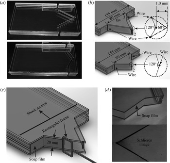
The ‘V’ shaped interface is created by an extended soap film technique in which thin wires are introduced as angular vertexes to connect adjacent sides of soap films. As sketched in figure 1(a), the interface framework is first manufactured using two Acrylic plates (3 mm in thickness) with a distance of 20 mm (i.e. the interface depth is 20 mm). Then, thin wires (0.2 mm in diameter) are introduced at positions 1, 2 and 3 as indicated in figure 1(b). The number of wires at each position depends on the angle between two adjacent soap films (Isenberg Reference Isenberg1992; Wang et al.
Reference Wang, Si and Luo2013). Specifically, for the corner with a large angle (
 $\unicode[STIX]{x1D703}\geqslant 120^{\circ }$
), only one wire is needed. For the corner with a small angle (
 $\unicode[STIX]{x1D703}\leqslant 60^{\circ }$
), three wires are used. For the corner with an intermediate angle (
 $60^{\circ }<\unicode[STIX]{x1D703}<120^{\circ }$
), two wires are employed. In the current interface configuration, only one wire is needed at positions 1 and 3 while the number of wires at position 2 depends upon the vertex angle
 $\unicode[STIX]{x1D703}$
. Note that using more than one wire will cause a slight rounding of the spike tips, as indicated in figure 1(b). The interface boundaries, as denoted by 1 and 3, contact the tube wall through another interface (the flat part) which will not be considered in the experiments. As a result, the effects of the tube wall on the interface evolution will be largely weakened. According to the expression provided by Morgan et al. (Reference Morgan, Aure, Stockero, Greenough, Cabot, Likhachev and Jacobs2012), the towed velocity induced by the shock tube wall is estimated to be of the order of
 $3.5~\text{m}~\text{s}^{-1}$
for the experiment duration, which is approximately 6 % of the interface velocity induced by the incident shock. Therefore, the boundary layer effect on the interface evolution is limited and can be neglected. In fact, given the experiment duration of 1.5 ms, temperature of 298 K and an incident shock Mach number of 1.2, the estimated boundary layer thickness is no more than 0.1 mm in the height direction, which is 0.5 % of the height. It should be mentioned that the interface considered in this work is not a periodic chevron one due to the existence of two flat parts, which will result in some differences of wave pattern near the wall compared with a periodic chevron one. Before generating interfaces, the framework edges should be properly wetted using the solution prepared (made of 78 % distilled water, 2 % sodium oleate and 20 % glycerine by mass). Afterwards, a rectangular frame with the soap film on its surface is pulled along the interface framework, as shown in figure 1(c), and then a ‘V’ shaped interface is formed. The schlieren image of the ‘V’ shaped interface formed is presented in figure 1(d) from which the initial flow field can be clearly identified. From our previous work (Zhai et al.
Reference Zhai, Wang, Si and Luo2014a
), good agreement between the experiments and two-dimensional numerical simulations was reached, and the three-dimensional effect of the initial interface was estimated to be smaller than 5 %, which showed that the initial interface can be regarded as two-dimensional. Because the initial conditions in the present experiment are very similar to the previous ones, the three-dimensional effect of the initial ‘V’ shaped interface can also be neglected. In this work, five ‘V’ shaped interfaces with different vertex angles (60
 $^{\circ }$
, 90
 $^{\circ }$
, 120
 $^{\circ }$
, 140
 $^{\circ }$
and 160
 $^{\circ }$
) are considered by fixing the initial interface height (
 $H_{0}$
) to 80 mm. For the current interface configuration, the initial amplitude (
 $a_{0}$
) is defined to be the total extent of the ‘V’ shaped interface, which is twice the usual amplitude for a single-mode interface. Accordingly, the wavelength (
 $\unicode[STIX]{x1D706}$
) in the ‘V’ shaped interface is taken as
 $\unicode[STIX]{x1D706}=2H_{0}$
. From simple geometry, the relationship among
 $a_{0}$
,
 $\unicode[STIX]{x1D706}$
and
 $\unicode[STIX]{x1D703}$
is given by
 $a_{0}/\unicode[STIX]{x1D706}=1/4\tan (\unicode[STIX]{x1D703}/2)$
. As can be found in table 1, a linear initial condition is satisfied only for the cases of
 $\unicode[STIX]{x1D703}=160^{\circ }$
and
 $140^{\circ }$
(
 $a_{0}/\unicode[STIX]{x1D706}<0.1$
).
The interface formation method. (a) Acrylic model used in experiments. (b) Arrangement of wires at the vertex for
 $\unicode[STIX]{x1D703}=60^{\circ }$
and
 $120^{\circ }$
. (c) Interface formation device. (d) The formed interface and the corresponding schlieren photograph.

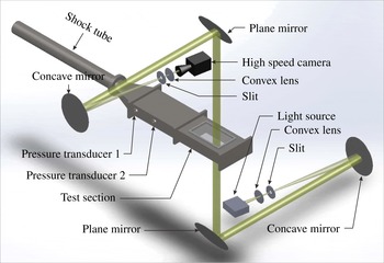
High-speed schlieren photography adopted in experiments.

Experimental parameters for all cases.

Experiments are conducted in a similar horizontal shock tube as in our previous work (Wang et al.
Reference Wang, Si and Luo2013; Zhai et al.
Reference Zhai, Wang, Si and Luo2014a
; Luo et al.
Reference Luo, Wang, Si and Zhai2015). The shock tube consists of a 1.7 m long driver section, a 3.9 m long driven section and a 1.0 m long test section. The rectangular cross-section of the test section is 155 mm
 $\times$
26 mm. The incident shock Mach number (
 $M$
) measured by piezoelectric transducers is 1.20
 $\pm$
0.01. Illuminated by a DC-regulated light source (DCR III, SCHOTT North America, Inc), the postshock flow field is recorded by the high-speed schlieren photograph as indicated in figure 2 with a high-speed video camera (FASTCAM SA5, Photron Limited). The detailed experimental parameters are listed in table 1. Prior to an experiment, air at the right side of interface should be removed and replaced by the test gas SF
 $_{6}$
. Therefore, the test section is first disconnected from the driven section and then tilted at an angle of
 ${\sim}$
20
 $^{\circ }$
to the horizontal plane. From the lower side of the test section, SF
 $_{6}$
is injected into the test section through a small hole. Because the density of air is much smaller than that of SF
 $_{6}$
, air in the test section is gradually exhausted and replaced by SF
 $_{6}$
. A gas concentration detector is placed at the upper side of the test section to ensure the purity of SF
 $_{6}$
in the test section. The gas concentration detector measures the concentration of the oxygen in air to determine the purity of the air. The measuring range is 0–25 % volume fraction, and the accuracy is 0.1 % volume fraction. In our experiments, when the concentration of oxygen in air is lower than 0.5 % volume fraction, it is considered that the air in the test section has been replaced by SF
 $_{6}$
completely. Once the concentration of SF
 $_{6}$
meets the requirement, the framework with a formed ‘V’ shaped interface is inserted into the test section slowly from its upper side. During insertion of the framework, SF
 $_{6}$
is continuously injected into the test section to ensure the purity of test gas. Another small hole is arranged at the lower side of the test section to release excess SF
 $_{6}$
. When the framework reaches the desired position, the two holes are sealed and the test section is connected to the driven section. This process lasts approximately 1 minute, and the SF
 $_{6}$
will be contaminated by air by approximately 10 % by mass.
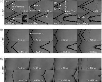
Schlieren sequences showing the evolution of a shocked ‘V’ shaped air/SF
 $_{6}$
interface for
 $\unicode[STIX]{x1D703}=60^{\circ }$
(a),
 $\unicode[STIX]{x1D703}=120^{\circ }$
(b) and
 $\unicode[STIX]{x1D703}=160^{\circ }$
(c). IS, incident shock; RS, refracted shock; TP, triple point; Lv, vortex spacing;
 $a_{0}$
, initial interface amplitude;
 $a$
, evolving interface amplitude;
 $H_{0}$
, initial interface height;
 $D_{S}$
, displacement of the upstream interface; RFS, reflected shock from the interface.

3 Results and discussion
3.1 Interface morphology and features
The evolution of the shocked interfaces is illustrated in figure 3. For all cases, the moment when the incident shock contacts the upstream interface is defined as the initial time (i.e.
 $t=0$
). It should be noted that only three schlieren sequences (
 $\unicode[STIX]{x1D703}=60^{\circ }$
, 120
 $^{\circ }$
and 160
 $^{\circ }$
) are shown because the results of
 $\unicode[STIX]{x1D703}=90^{\circ }$
and 140
 $^{\circ }$
are similar to those of
 $\unicode[STIX]{x1D703}=60^{\circ }$
and 120
 $^{\circ }$
, respectively, and are omitted here. When an incident shock (IS) encounters the inclined air/SF
 $_{6}$
interface, a refracted shock wave (RS) generates in the SF
 $_{6}$
gas and, simultaneously, a reflected shock wave (RFS) propagates back into the air. The interaction of the refracted shocks from the upper and lower half-planes results in two new shocks (
 $S_{1}$
in figure 3
a at
 $t=171~\unicode[STIX]{x03BC}\text{s}$
) and two triple points (TP). Compressed by the incident shock, the interface begins to bend towards the symmetry axis (figure 3
a at
 $t=171~\unicode[STIX]{x03BC}\text{s}$
). Due to baroclinic vorticity deposition caused by the misalignment of density and pressure gradients, vortices form on the interface and one well-organized vortex pair is visible at the interface vertex (figure 3
a at
 $t=531~\unicode[STIX]{x03BC}\text{s}$
). Note that in previous numerical work (Hahn et al.
Reference Hahn, Drikakis, Youngs and Williams2011; McFarland et al.
Reference Mcfarland, Reilly, Black, Greenough and Ranjan2015) and experimental work (Holder & Barton Reference Holder, Barton and Dalziel2004), these obvious vortices are not visible. In the simulation of McFarland et al. (Reference Mcfarland, Reilly, Black, Greenough and Ranjan2015), a 1.2 cm diffusion thickness was adopted, and we believe that the amplitude of vorticity created on the diffusion interface by the baroclinic torque will be significantly reduced. In the simulation of Hahn et al. (Reference Hahn, Drikakis, Youngs and Williams2011), in order to compare with the experimental results of Holder & Barton (Reference Holder, Barton and Dalziel2004), random multi-mode perturbations were added in their initial conditions to determine the effect of supports. This will also decrease the amplitude of baroclinic vorticity deposited on the interface. Furthermore, the central obtuse angle in the simulation and experiment is 157
 $^{\circ }$
so that the baroclinic torque is too weak to generate obvious vortices. In the present work, as the vertex angle increases from 60
 $^{\circ }$
to 120
 $^{\circ }$
and further to 160
 $^{\circ }$
, the vortices are gradually weakened as can be found at
 $t=1161~\unicode[STIX]{x03BC}\text{s}$
for
 $\unicode[STIX]{x1D703}=60^{\circ }$
, and
 $t=1505~\unicode[STIX]{x03BC}\text{s}$
for
 $\unicode[STIX]{x1D703}=120^{\circ }$
and
 $t=1697~\unicode[STIX]{x03BC}\text{s}$
for
 $\unicode[STIX]{x1D703}=160^{\circ }$
. The wires adopted to connect the interface at each vertex may introduce perturbations on the interface in the vicinity of the vertex. However, the wires cannot generate large effects on the interface far away from them. Moreover, for
 $\unicode[STIX]{x1D703}=120^{\circ }$
and 160
 $^{\circ }$
, the numbers of wires are the same, and the only difference among these two cases is the baroclinic torque caused by the different angle. Therefore, it can be concluded that a discontinuous interface without supports will be beneficial to generate vortices on the interface, and the baroclinic torque is the primary factor that results in the vorticity. As time proceeds, the vortex pair increases in scale and vortices on the interface become apparent (figure 3
a at
 $t=1011~\unicode[STIX]{x03BC}\text{s}$
). At late stages, the flat part of the initial interface (connected directly to the tube wall) deforms, which is not induced by the incident shock but by other shocks, such as the refracted shocks or reflected shocks from the wall, which are not parallel to the flat interface, and influences the evolution of the inclined interface adjacent to it (figure 3
a at
 $t=1011~\unicode[STIX]{x03BC}\text{s}$
). As vertex angle increases, vorticity amplitude decreases, vortices on the interface become less noticeable for
 $\unicode[STIX]{x1D703}=120^{\circ }$
in figure 3(b) and are hardly observable for
 $\unicode[STIX]{x1D703}=160^{\circ }$
in figure 3(c).
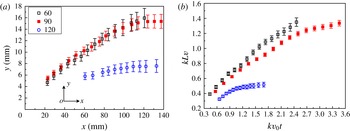
The characteristic of the vortex measured from the schlieren sequences for the three cases (
 $\unicode[STIX]{x1D703}=60^{\circ }$
, 90
 $^{\circ }$
and 120
 $^{\circ }$
). (a) Variation of the vortex core position. (b) Dimensionless vortex spacing versus dimensionless time.

Vorticity plays a leading role in enhancing the mixing between gases and its formation generally indicates the transition of the perturbation growth from a linear to a nonlinear phase. Figure 4 presents the trajectory of the vortex core, along with the variation of normalized vortex spacing for
 $\unicode[STIX]{x1D703}=60^{\circ }$
, 90
 $^{\circ }$
and 120
 $^{\circ }$
. The initial interface vertex is defined as the origin of coordinates and the vortex spacing Lv, defined in figure 3, is normalized by
 $1/k$
with
 $k$
the wavenumber (
 $k=2\unicode[STIX]{x03C0}/\unicode[STIX]{x1D706}$
). The dimensionless time is
 $kv_{0}t$
with
 $v_{0}$
the initial linear growth rate for different cases. The coordinates of the vortex core from the upper half-plane presented in figure 4(a) are obtained by taking the average value of the vortex cores in the upper and lower half-planes. The error bars represent uncertainty of the manual measurement because of the interface thickness in the vicinity of the vortex core. At early stages, the vortex pair grows with a velocity in the spanwise direction. Finally, a fully developed vortex pair is observed and the vortex cores move only in the streamwise direction. As a result, the vortex spacing first experiences a growth phase and then becomes saturated, as shown in figure 4(b). For the
 $\unicode[STIX]{x1D703}=60^{\circ }$
case, more vorticity deposits on the interface, and, therefore, more time is needed for the vortex pair to saturate and the scale of the vortex pair is larger.
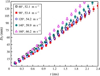
The behaviour of vortex pair derived from the interface vertex will influence the movement of the upstream interface. Figure 5 provides the time variation of the upstream interface displacement
 $D_{S}$
(the distance from the initial interface vertex to the evolving upstream interface, as indicated in figure 3) for five cases, and the error bars represent the experimental uncertainty. Velocities of the upstream interface calculated from the linear fitting are also given in the figure, which clearly state that, as the vertex angle increases, the upstream interface moves faster. For an air/SF
 $_{6}$
interface, the velocity induced by vorticity is generally in the opposite direction to the postshock flow velocity. Consequently, as the vertex angle increases, the inverted velocity induced by vorticity decreases, resulting in the faster movement of the upstream interface. Note that for smaller perturbations, i.e. large
 $\unicode[STIX]{x1D703}$
, the velocities listed in the inset of figure 5 approach the jump velocity for a flat interface, which is numerically given as
 $71.8~\text{m}~\text{s}^{-1}$
.
Time variation of the upstream interface displacement.

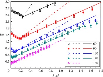
Comparison of interface width growth rate in the linear stage between the experiments and theoretical models. Symbols: experiments; dashed lines: the impulsive model (Richtmyer Reference Richtmyer1960); solid lines: the modified model (Rikanati et al. Reference Rikanati, Oron, Sadot and Shvarts2003).

3.2 Linear stage of interface width growth
Figure 6 shows the variation of interface width (
 $ka$
) versus time in a dimensionless form. The interface width first decreases due to the shock compression and then increases with time. A nearly linear growth rate is observed for 160
 $^{\circ }$
, while for
 $\unicode[STIX]{x1D703}=60^{\circ }$
, 90
 $^{\circ }$
, 120
 $^{\circ }$
and 140
 $^{\circ }$
, a linear stage followed by a nonlinear stage is found. For
 $\unicode[STIX]{x1D703}=160^{\circ }$
, due to the limitation of the visualizing windows, the interface moves out of the field of view before nonlinear growth occurs. It is reasonable to observe that the durations of the linear growth rate in the cases of
 $\unicode[STIX]{x1D703}=160^{\circ }$
and 140
 $^{\circ }$
are longer because only these two cases meet the requirement of the linear regime (
 $a_{0}/\unicode[STIX]{x1D706}<0.1$
). However, for the other three cases, which violate the requirement of the linear regime (
 $a_{0}/\unicode[STIX]{x1D706}>0.1$
), an obvious linear phase still exists for each case at the early stage after the compression phase because the current initial interface can be treated as a spike. As
 $a_{0}/\unicode[STIX]{x1D706}$
increases, secondary compressible effects (shocks reflected from the initial wall) become stronger and more vorticity deposits on the interface, resulting in the earlier appearance of nonlinear growth of the interface width.
As pointed out by Mikaelian (Reference Mikaelian1993), the initial ‘V’ shaped interface can be expressed in the form of a Fourier expansion. Firstly the shape function is defined as
 $$\begin{eqnarray}\displaystyle y(x)=\left\{\begin{array}{@{}ll@{}}2x/\unicode[STIX]{x03C0} & (0<x<\unicode[STIX]{x03C0}/2)\\ 2-2x/\unicode[STIX]{x03C0} & (\unicode[STIX]{x03C0}/2<x<\unicode[STIX]{x03C0}),\end{array}\right. & & \displaystyle\end{eqnarray}$$
then
 $y(x)$
can be expanded in Fourier series,
 $$\begin{eqnarray}\displaystyle y(x)=\frac{8}{\unicode[STIX]{x03C0}^{2}}\left\{\sin x-\frac{\sin 3x}{3^{2}}+\frac{\sin 5x}{5^{2}}-\frac{\sin 7x}{7^{2}}+\frac{\sin 9x}{9^{2}}-\cdots \right\}. & & \displaystyle\end{eqnarray}$$
It can be concluded that the fundamental mode, which has a wavelength equal to the opening of the ‘V’, contains
 ${\sim}$
81 % (
 $8/\unicode[STIX]{x03C0}^{2}$
) of the mode. The other infinitely many shorter modes make up the remaining 19 %. In other words, 81 % of the mode almost determines the mixing width of the interface with a small amplitude in the linear phase. Based on this consideration, we can approximately estimate the growth rate of the ‘V’ shaped interfaces by the classical impulsive model. The growth rate for a sinusoidal interface with a small amplitude in the linear regime can be described by the classical impulsive model (Richtmyer Reference Richtmyer1960) as:
 $$\begin{eqnarray}\displaystyle a=a_{0}^{+}(1+\unicode[STIX]{x0394}vkA^{+}t)\quad (0<t), & & \displaystyle\end{eqnarray}$$
where
 $\unicode[STIX]{x0394}v$
,
 $a_{0}^{+}$
and
 $A^{+}$
are, respectively, interface velocity jump, postshock initial amplitude and postshock Atwood number (defined as
 $(\unicode[STIX]{x1D70C}_{SF_{6}}^{+}-\unicode[STIX]{x1D70C}_{air}^{+})/(\unicode[STIX]{x1D70C}_{SF_{6}}^{+}+\unicode[STIX]{x1D70C}_{air}^{+})$
with
 $\unicode[STIX]{x1D70C}_{SF_{6}}^{+}$
and
 $\unicode[STIX]{x1D70C}_{air}^{+}$
being the densities of SF
 $_{6}$
and air after the shock impact, respectively). The predictions of the interface width from the impulsive model after the compression phase for five cases are denoted by dashed lines in figure 6. Overall poor agreements between the experimental and theoretical results are found for the cases of
 $\unicode[STIX]{x1D703}=60^{\circ }$
, 90
 $^{\circ }$
and 120
 $^{\circ }$
, because the ‘V’ shaped interfaces in these three cases have large amplitudes and are not pure sinusoidal. Relatively better agreement is found for the cases of
 $\unicode[STIX]{x1D703}=160^{\circ }$
and 140
 $^{\circ }$
, which have small initial amplitudes.
For the evolution of RMI on a sinusoidal interface with a high initial amplitude, according to the work of Velikovich & Dimonte (Reference Velikovich and Dimonte1996), Dimonte & Ramaprabhu (Reference Dimonte and Ramaprabhu2010) proposed a model with a Padé approximation,
 $$\begin{eqnarray}\displaystyle v_{0}=\frac{v_{lin}}{1+(ka_{0}/3)^{4/3}}. & & \displaystyle\end{eqnarray}$$
In the model,
 $v_{lin}$
stands for the growth rate predicted by the classical impulsive model (Richtmyer Reference Richtmyer1960). Further, Rikanati et al. (Reference Rikanati, Oron, Sadot and Shvarts2003) proposed a similar theory applicable for both sinusoidal and ‘V’ shaped interfaces with a high initial amplitude. A reduction factor (
 $R$
) was introduced to predict the velocity of interface with a high initial amplitude, which can be described by
 $$\begin{eqnarray}\displaystyle & \displaystyle R=u_{0}(a)/u_{0}^{lin}(a), & \displaystyle\end{eqnarray}$$
 $$\begin{eqnarray}\displaystyle & \displaystyle u_{0}(a)=-Re\left[f\int _{0}^{\unicode[STIX]{x1D706}}\frac{\sin [\unicode[STIX]{x1D6FC}^{-}]}{\cos [\unicode[STIX]{x1D6FC}^{+}]}\times \cot \{\unicode[STIX]{x03C0}/2[-x+\text{i}a_{0}f_{p}(1-y(x))]/\unicode[STIX]{x1D706}\}\,\text{d}x\right], & \displaystyle\end{eqnarray}$$
 $$\begin{eqnarray}\displaystyle & \displaystyle u_{0}^{lin}(a)=-aRe\left[-f\int _{0}^{\unicode[STIX]{x1D706}}\unicode[STIX]{x03C0}\sin (\unicode[STIX]{x03C0}x/\unicode[STIX]{x1D706})\cot (-\unicode[STIX]{x03C0}/2x\unicode[STIX]{x1D706})\,\text{d}x\right]. & \displaystyle\end{eqnarray}$$
 $u_{0}$
is the initial tip velocity induced due to a general periodic vorticity distribution on an interface (Baker, Meiron & Orszag Reference Baker, Meiron and Orszag1980) and
 $u_{0}^{lin}$
is the tip velocity obtained from the impulsive model.
 $f_{p}$
is a factor given by
 $f_{p}=(v_{s}-\unicode[STIX]{x0394}v)/v_{s}$
with
 $v_{s}$
the incident shock velocity.
 $y(x)$
is the shape function of the initial interface and during the shock–interface interaction,
 $y^{+}(x)=f_{p}y^{-}(x)$
, in which ‘
 $-$
’ and ‘
 $+$
’ represent the preshock and postshock states, respectively.
 $\unicode[STIX]{x1D6FC}^{\pm }=\arctan (\text{d}y^{\pm }(x)/\text{d}x)$
stand for the angles between the incident shock and interface before and after the shock impact, respectively.
 $f$
is a function relating to the vorticity per unit length deposited on a straight interface by an oblique shock wave (Samtaney & Zabusky Reference Samtaney and Zabusky1994), and, for angles smaller than the Mach reflection critical angle, deposited vorticity per unit length can be given as
 $$\begin{eqnarray}\displaystyle \frac{\text{d}\unicode[STIX]{x1D6E4}}{\text{d}s}=f(M,\unicode[STIX]{x1D70C}_{1},\unicode[STIX]{x1D70C}_{2},\unicode[STIX]{x1D6FE}_{1},\unicode[STIX]{x1D6FE}_{2},p_{1},p_{2})\sin \unicode[STIX]{x1D6FC}+O(\sin ^{3}\unicode[STIX]{x1D6FC}). & & \displaystyle\end{eqnarray}$$
In the present work, reduction factors
 $R$
for different initial amplitudes are calculated according to (3.5), and the values are listed in table 2. With the reduction factor, a modified model to predict the growth rate of interface width for a ‘V’ shaped initial interface is given by
 $$\begin{eqnarray}\displaystyle a=a_{0}^{+}+a_{0}^{+}A^{+}\unicode[STIX]{x0394}vkt\ast R. & & \displaystyle\end{eqnarray}$$
Based on the modified linear model (3.9), the interface width growth in the linear stage for each case is theoretically obtained, as presented by solid lines in figure 6. Comparison between the experimental and theoretical results shows that the modified linear model can describe the interface evolution quite well in the linear phase.
The reduction factor
 $R$
and the initial linear growth rate
 $v_{0}$
calculated from the modified linear model (3.10).

According to (3.9), the width growth rate
 $v_{0}$
can be obtained through the time derivative of the width
 $a$
, and can be described by
 $$\begin{eqnarray}\displaystyle v_{0}=\frac{\text{d}a}{\text{d}t}=a_{0}^{+}A^{+}\unicode[STIX]{x0394}vk\ast R. & & \displaystyle\end{eqnarray}$$
For these five cases, the growth rates of the interface width in the linear stage are calculated by (3.10) and the values are listed in table 2. It can be observed that a larger divergence in the interface width growth rate exists, distinguishing the cases of
 $\unicode[STIX]{x1D703}=140^{\circ }$
and 160
 $^{\circ }$
from the other three cases. This difference in the interface width growth rate was also found in previous work (McFarland et al.
Reference Mcfarland, Greenough and Ranjan2013, Reference Mcfarland, Greenough and Ranjan2014a
,Reference Mcfarland, Reilly, Creel, Mcdonald, Finn and Ranjan
b
). McFarland et al. (Reference Mcfarland, Greenough and Ranjan2013) reported in their numerical work that a growth regime change occurs near a vertex angle of 160
 $^{\circ }$
and they attributed this change to secondary compressible effects. Although secondary compressible effects are difficult to identify in the current experiments, the present results provide an experimental evidence of the regime change and consequently verify the numerical viewpoint suggested by McFarland et al. (Reference Mcfarland, Greenough and Ranjan2013). Based on our experimental results, it is further revealed that the high initial amplitude causes the secondary compressible effects and, subsequently, the change of the growth rate at a certain vertex angle.
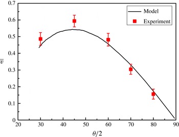
Variation of interface width growth rate with initial amplitude from experiment (symbols) and model (line).

We can also find that the interface width growth rate in the linear stage experiences an increase and then a decrease as the vertex angle increases (i.e. initial perturbation amplitude decreases). A similar conclusion has been reported by Dell, Stellingwerf & Abarzhi (Reference Dell, Stellingwerf and Abarzhi2015) for an initial sinusoidal perturbation in their numerical simulations. They found that, for a given shock strength and density ratio, the initial growth rate of the interface width is a non-monotone function of the initial perturbation amplitude, i.e. increasing for small initial amplitudes and decreasing for very large initial amplitudes. The non-monotonicity of interface width growth rate
 $v_{0}$
can be due to a combination of the geometric effect and the effect of secondary shocks.
In order to describe the relationship between the linear growth rate
 $v_{0}$
and the initial vertex angle
 $\unicode[STIX]{x1D703}$
, (3.10) is rewritten as
 $$\begin{eqnarray}\displaystyle v_{0}=\frac{\text{d}a}{\text{d}t}=\frac{\unicode[STIX]{x03C0}a_{0}^{+}}{2a_{0}}A^{+}R\cot (\unicode[STIX]{x1D703}/2)\unicode[STIX]{x0394}v. & & \displaystyle\end{eqnarray}$$
According to (3.11), given the initial shock Mach number and the Atwood number, the width growth rate
 $v_{0}$
is a function of the vertex angle
 $\unicode[STIX]{x1D703}$
only because the reduction factor
 $R$
can also be expressed only by
 $\unicode[STIX]{x1D703}$
. Here, we define
 $\overline{v}=2v_{0}a_{0}/(\unicode[STIX]{x03C0}Aa_{0}^{+}\unicode[STIX]{x0394}v)=R\cot (\unicode[STIX]{x1D703}/2)$
. From this expression, the variation of
 $\overline{v}$
with the vertex angle
 $\unicode[STIX]{x1D703}$
can be theoretically solved, as shown in figure 7, together with the experimental values. It is found that the interface width growth rate is indeed a non-monotone function of the initial vertex angle, verifying the numerical viewpoint proposed by Dell et al. (Reference Dell, Stellingwerf and Abarzhi2015) through both theoretical and experimental methods. Dell et al. (Reference Dell, Stellingwerf and Abarzhi2015) also pointed out that the value of
 $(a_{0}/\unicode[STIX]{x1D706})_{max}$
, corresponding to the maximum growth rate, is between 0.2 and 0.4 and it depends only slightly on the shock Mach number and Atwood number. From the present work, the maximum growth rate occurs near
 $\unicode[STIX]{x1D703}=90^{\circ }$
, corresponding to a value of
 $a_{0}/\unicode[STIX]{x1D706}$
of 0.25, which also agrees well with the numerical results (Dell et al.
Reference Dell, Stellingwerf and Abarzhi2015).
Comparing (3.4) with (3.10), the reduction factor is therefore
 $1/[1+(ka_{0}/3)^{4/3}]$
. Since
 $v_{lin}$
is proportional to
 $ka_{0}$
, (3.4) can be rewritten as
 $$\begin{eqnarray}\displaystyle v_{0}=\frac{Cka_{0}}{1+(ka_{0}/3)^{4/3}}, & & \displaystyle\end{eqnarray}$$
where
 $C$
is a constant. From (3.12),
 $v_{0}$
reaches its peak at
 $ka_{0}=3^{7/4}=6.84$
, i.e.
 $a_{0}/\unicode[STIX]{x1D706}\approx 1.09$
, which is too large compared with the experimental result. Therefore, (3.4) is not applicable to prediction of the width linear growth rate for the current interface configuration. Besides (3.4), Dimonte & Ramaprabhu (Reference Dimonte and Ramaprabhu2010) also provided a reduction factor as a fit to the spike evolution (Buttler et al.
Reference Buttler, Oró, Preston, Mikaelian, Cherne, Hixson, Mariam, Morris, Stone, Terrones and Tupa2012), which can be written as:
 $$\begin{eqnarray}\displaystyle v_{0}=\frac{Cka_{0}}{1+(ka_{0}/2)^{2}}. & & \displaystyle\end{eqnarray}$$
This expression has its maximum at
 $ka_{0}=2$
, i.e.
 $a_{0}/\unicode[STIX]{x1D706}\approx 0.32$
, which is much closer to the experimental result (
 $a_{0}/\unicode[STIX]{x1D706}\approx 0.25$
) and agrees well with the conclusion reached by Dell et al. (Reference Dell, Stellingwerf and Abarzhi2015).
3.3 Nonlinear stage of interface width growth
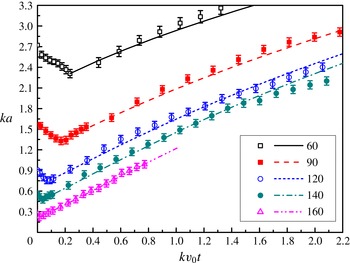
Comparison of dimensionless interface width between the experiments and theoretical predictions in linear and nonlinear phases. Symbols represent the experimental results and lines represent the theoretical results.

In the nonlinear phase, Dimonte & Ramaprabhu (Reference Dimonte and Ramaprabhu2010) have proposed a model (DR model) to fit the linear, nonlinear and asymptotic behaviours of the separate bubble and spike evolution. The DR model can be expressed as
 $$\begin{eqnarray}\displaystyle & \displaystyle v_{b/s}=v_{0}\frac{1+(1\mp |A^{+}|)\unicode[STIX]{x1D70F}}{1+C_{bu/sp}\unicode[STIX]{x1D70F}+(1\mp |A^{+}|)F_{bu/sp}\unicode[STIX]{x1D70F}^{2}}, & \displaystyle\end{eqnarray}$$
 $$\begin{eqnarray}\displaystyle & \displaystyle C_{b/s}=\frac{4.5\pm |A^{+}|+(2\mp |A^{+}|)|ka_{0}|}{4}, & \displaystyle\end{eqnarray}$$
 $$\begin{eqnarray}\displaystyle & \displaystyle F_{b/s}=1\pm |A^{+}|, & \displaystyle\end{eqnarray}$$
 $v_{b/s}$
and
 $|A^{+}|$
are the growth rate of the bubble or spike and the absolute value of the Atwood number after the shock.
 $C_{b/s}$
and
 $F_{b/s}$
are functions determined by the Atwood number and initial amplitude and wavenumber. Given that the initial linear growth rate
 $v_{0}$
is calculated from the modified linear model (3.10) (the values of
 $v_{0}$
for cases are listed in table 2), then the width growth rate is estimated by the DR model. The comparison of the estimations with the experiments is provided in figure 8. As stated earlier, for
 $\unicode[STIX]{x1D703}=160^{\circ }$
the interface has moved out of the flow field before the nonlinear growth occurs, while for
 $\unicode[STIX]{x1D703}=60^{\circ }$
, 90
 $^{\circ }$
, 120
 $^{\circ }$
and 140
 $^{\circ }$
, a nearly linear growth is followed by a nonlinear phase during the time studied. During the nonlinear stage, the interface widths increase in the form of a power law and coincide well with the theoretical predictions. In conclusion, the DR model can well predict the interface width during the linear and early nonlinear stages. As mentioned earlier, the interface considered in the present work is not a periodic chevron one due to the existence of two flat parts. However, Fourier expansion shows that the model seems to work well, which indicates that the flat portions of the interface can be neglected. In other word, the interface considered in the present study behaves like a pure chevron interface.
4 Conclusions
A soap film technique is adopted to create a discontinuous ‘V’ shaped air/SF
 $_{6}$
interface for shock refraction and RMI studies. The interface formed is free of supports and can be well controlled. Evolution of a shocked ‘V’ shaped air/SF
 $_{6}$
interface is recorded by high-speed schlieren photography and the effects of the initial interface amplitude over wavelength on the mixing width are highlighted.
The evolution of shocked ‘V’ shaped interfaces is sensitive to the vertex angle. For small vertex angles, more vorticity is produced on the interface, resulting in the formation of many vortices. Specifically, a noticeable vortex pair derives from the interface vertex, influencing the interface movement. For large vertex angles, only slight deformation of the interface is observed after the shock impact because less vorticity is created. Quantitatively, the position and vortex spacing of the vortex pair from the interface vertex are obtained. The vortex pair grows both in the streamwise and spanwise directions from the beginning, and subsequently becomes saturated. The interface width growth rate is experimentally measured and the results reveal that a regime change occurs in the interface width growth rate near a vertex angle of 160
 $^{\circ }$
corresponding to a linear initial perturbation, which provides an experimental evidence for the previous numerical result (McFarland et al.
Reference Mcfarland, Greenough and Ranjan2013). Besides, the interface widths in the linear stage from experiments are compared with those predicted by the classical impulsive model and a modified linear model. Overall, the impulsive model can reflect the width growth rate for small amplitudes but it is invalid for high initial amplitudes. The modified linear model is proven to be effective for predicting width growth rate when the initial amplitude is large. From the modified linear model and experiments, we find a non-monotone dependence of the width growth rate in the linear phase on the initial perturbation amplitude. As the initial amplitude increases, the growth rate increases first and then decreases. A similar conclusion was also reported by Dell et al. (Reference Dell, Stellingwerf and Abarzhi2015) for a sinusoidal interface, and our work, for the first time, provides experimental and theoretical evidence for this numerical viewpoint. The corresponding value of the initial amplitude obtained from the experiment and model when the maximum growth rate is reached also agrees with the numerical result. In the nonlinear stage, the general behaviour of the interface width growth, i.e. a linear growth followed by slowing down, is well captured by the nonlinear model proposed by Dimonte & Ramaprabhu (Reference Dimonte and Ramaprabhu2010).
As pointed out by McFarland et al. (Reference Mcfarland, Reilly, Black, Greenough and Ranjan2015), in their numerical results the boundary layer has a significant effect on the development of the inclined interface. In this work, although the ‘V’ shaped interface is not a periodic chevron one, it presents important references for investigating the evolution of an inclined interface. However, due to the limitations of the experimental technique, the late time images of the entire shock tube domain extending to the boundaries cannot be acquired. As a result, in our experimental duration, the effects created by the flat boundaries cannot be evaluated and will be addressed in future work.
Acknowledgements
We thank Professor K. O. Mikaelian for the fruitful discussions on the theoretical modelling. This work is supported by the National Natural Science Foundation of China (11302219, 11272308, NSAF U1530103).