1 Introduction
Fluid flows are characterized by high-dimensional, nonlinear dynamics that gives rise to rich structures. Despite this apparent complexity, the dynamics often evolves on a low-dimensional attractor defined by a few dominant coherent structures that contain significant energy or are useful for control (Holmes et al. Reference Holmes, Lumley, Berkooz and Rowley2012). Given this property, one might aim to derive or identify reduced-order models that reproduce qualitatively and quantitatively the dynamics of the full system. Over the past decades, identifying robust, accurate and efficient reduced-order models has thus become a central challenge in fluid dynamics and closed-loop flow control (Fabbiane et al. Reference Fabbiane, Semeraro, Bagheri and Henningson2014; Brunton & Noack Reference Brunton and Noack2015; Sipp & Schmid Reference Sipp and Schmid2016; Rowley & Dawson Reference Rowley and Dawson2017).
Many traditional model reduction techniques are analytical. They rely on prior knowledge of the Navier–Stokes equations and the existence of a high-fidelity solver to project onto an orthogonal basis of modes, resulting in a dynamical system in terms of the coefficients of this expansion basis. These modes may come from a classical expansion, such as Fourier modes, or they may be data-driven, as in the proper orthogonal decomposition (POD) (Sirovich Reference Sirovich1987; Berkooz, Holmes & Lumley Reference Berkooz, Holmes and Lumley1993). In the latter case, the model reduction may be considered a hybrid approach, mixing knowledge of the physics with empirical modes obtained from measurement data. Control-theoretic extensions, such as balanced POD (BPOD) (Willcox & Peraire Reference Willcox and Peraire2002; Rowley Reference Rowley2005), have also been widely applied for closed-loop flow control (Ilak & Rowley Reference Ilak and Rowley2008; Bagheri, Brandt & Henningson Reference Bagheri, Brandt and Henningson2009; Illingworth, Morgans & Rowley Reference Illingworth, Morgans and Rowley2010). Although such approaches to model reduction have been widely successful for linear systems, as described in the recent review by Rowley & Dawson (Reference Rowley and Dawson2017) and references therein, they have been applied with only limited success to obtain low-order approximations of nonlinear systems, mostly on flow oscillators. One can cite for instance the seminal work of Noack et al. (Reference Noack, Afanasiev, Morzynski, Tadmor and Thiele2003) and Tadmor et al. (Reference Tadmor, Lehmann, Noack and Morzyński2010) wherein the authors have shown that such reduced-order models obtained from a Galerkin projection can reproduce the transients and nonlinear dynamics of the von Kármán vortex shedding past a two-dimensional cylinder, provided the projection basis includes a shift mode quantifying the distortion between the linearly unstable base flow and marginally stable mean flow. Recently, Semaan et al. (Reference Semaan, Kumar, Burnazzi, Tissot, Cordier and Noack2016) have extended this reduced-order modelling strategy to include the effect of control actuation for the flow around a high-lift configuration airfoil.
In contrast, data-driven approaches are becoming increasingly popular and encompass a variety of different techniques such as the eigensystem realization algorithm (ERA) (Juang & Pappa Reference Juang and Pappa1985), dynamic mode decomposition (DMD) (Rowley et al. Reference Rowley, Mezić, Bagheri, Schlatter and Henningson2009; Schmid Reference Schmid2010; Kutz et al. Reference Kutz, Brunton, Brunton and Proctor2016), Koopman theory (Mezić Reference Mezić2005, Reference Mezić2013) and variants (Tu et al. Reference Tu, Rowley, Luchtenburg, Brunton and Kutz2014; Williams, Kevrekidis & Rowley Reference Williams, Kevrekidis and Rowley2015), cluster reduced-order modelling (CROM) (Kaiser et al. Reference Kaiser, Noack, Cordier, Spohn, Segond, Abel, Daviller, Osth, Krajnovic and Niven2014), NARMAX (Glaz, Liu & Friedmann Reference Glaz, Liu and Friedmann2010; Zhang et al. Reference Zhang, Wang, Ye and Quan2012; Billings Reference Billings2013; Semeraro et al. Reference Semeraro, Lusseyran, Pastur and Jordan2017) and network analysis of fluids (Nair & Taira Reference Nair and Taira2015). Advances in machine learning are also greatly expanding the ability to extract governing dynamics purely from data. Neural networks have long been used for flow modelling (Milano & Koumoutsakos Reference Milano and Koumoutsakos2002; Zhang & Duraisamy Reference Zhang and Duraisamy2015) and control (Lee et al. Reference Lee, Kim, Babcock and Goodman1997), and recently deep neural networks (Krizhevsky, Sutskever & Hinton Reference Krizhevsky, Sutskever, Hinton, Pereira, Burges, Bottou and Weinberger2012) have been used for Reynolds averaged turbulence modelling (Ling, Kurzawski & Templeton Reference Ling, Kurzawski and Templeton2016; Kutz Reference Kutz2017). However, many approaches in machine learning, such as neural networks, are prone to overfitting, do not yield interpretable models, and make it difficult to incorporate known physical constraints.
Advanced regression methods from statistics, such as genetic programming or sparse regression, are driving new algorithms that identify parsimonious nonlinear dynamics from measurements of complex systems. Bongard & Lipson (Reference Bongard and Lipson2007) and Schmidt & Lipson (Reference Schmidt and Lipson2009) introduced nonlinear system identification based on genetic programming, which has been used in numerous practical applications in aerospace engineering, the petroleum industry and in finance. More recently, Brunton, Proctor & Kutz (Reference Brunton, Proctor and Kutz2016a ) have proposed a system identification approach based on sparse regression known as the sparse identification of nonlinear dynamics (SINDy). Following the principle of Ockham’s razor, the SINDy algorithm rests on the assumption that there are only a few important terms that govern the dynamics of a given system, so that the equations are sparse in the space of possible functions. Sparse regression is then used to determine the fewest terms in a dynamical system required to accurately represent the data. The resulting models are parsimonious, balancing model complexity with descriptive power while avoiding overfitting and remaining interpretable.
Many of these regression techniques can be recast into a minimization problem and their solution can be obtained using efficient algorithms available in libraries such as CVXOPT (Andersen, Dahl & Vandenberghe Reference Andersen, Dahl and Vandenberghe2013). However, a major drawback of regression-based methods is the possible loss of existing symmetries in the governing equations which may otherwise be included in the physics-based Galerkin projection methods described previously (Noack, Morzynski & Tadmor Reference Noack, Morzynski and Tadmor2011; Balajewicz, Dowell & Noack Reference Balajewicz, Dowell and Noack2013; Carlberg, Tuminaro & Boggs Reference Carlberg, Tuminaro and Boggs2015; Schlegel & Noack Reference Schlegel and Noack2015). A notable exception is the physics-constrained multi-level quadratic regression used to identify models in climate and turbulence (Majda & Harlim Reference Majda and Harlim2012). Including energy-preserving constraints is known to improve the long-time stability and performance of nonlinear models, while standard Galerkin projection methods often suffer from stability issues (Carlberg, Barone & Antil Reference Carlberg, Barone and Antil2017). Starting from the original SINDy algorithm (Brunton et al. Reference Brunton, Proctor and Kutz2016a ), we propose in this work a new implementation of the algorithm which allows the user to include physical constraints such as energy-preserving nonlinearities or to enforce symmetries in the identified equations. The resulting algorithm relies on the use of constrained least-squares (Golub & Van Loan Reference Golub and Van Loan2012) to incorporate additional constraints in the SINDy algorithm for the sparse identification of the low-dimensional dynamical system. The ability of the present approach, hereafter named sparse Galerkin regression, is demonstrated on two different flow configurations: the emblematic two-dimensional cylinder flow and the shear-driven cavity flow. We also show that including higher-order nonlinearities in the regression improves the stability and accuracy of resulting models, capturing the effect of truncated low-energy modes on the dynamics of high-energy modes.
The manuscript is organized as follows: § 2.1 provides the reader with a quick introduction to the original SINDy algorithm, while the new algorithm is presented in § 2.2. The physical constraints used in this work are discussed in § 3, while the two flow configurations considered herein are presented in § 4. The different low-dimensional systems identified are compared against standard Galerkin projection in § 5. Finally, § 6 summarizes our key findings and provides the reader with possible extensions to this work.
2 Constrained sparse identification
Here we discuss the core mathematical and algorithmic framework used to identify nonlinear reduced-order models from data. The proposed Galerkin regression method is based on a modified version of the sparse identification of nonlinear dynamics (SINDy) method (Brunton et al. Reference Brunton, Proctor and Kutz2016a ). The original SINDy algorithm is introduced in § 2.1, and the modifications to include physical constraints, such as energy conservation, known eigenvalues or symmetries, are discussed in § 2.2. Implementation details for both algorithms are presented to promote reproducibility; in addition, code is freely available online (https://github.com/loiseaujc/SINDy). Specific constraints that are used to enforce energy conservation are derived later in § 3.
2.1 Sparse identification of nonlinear dynamics (SINDy)
Identifying dynamical systems from data has been a central challenge in mathematical physics, with a particularly rich history in fluid dynamics. Typically, the structure of the system identified is either constrained via prior knowledge of the governing equations, as in Galerkin projection, or a small handful of heuristic models are posited and parameters are optimized to match the data. Simultaneously identifying the structure and parameters of a model from data is considerably more challenging, as there are combinatorially many possible model structures. The sparse identification of nonlinear dynamics algorithm (Brunton et al. Reference Brunton, Proctor and Kutz2016a ) bypasses the intractable brute force search through all possible model structures, leveraging the observation that many dynamical systems
 $$\begin{eqnarray}\dot{\boldsymbol{x}}=\boldsymbol{f}(\boldsymbol{x})\end{eqnarray}$$
have dynamics
 $\boldsymbol{f}$
that is sparse in the space of possible right-hand side functions. It is then possible to solve for the relevant terms that are active in the dynamics using a convex
 $\ell _{1}$
-regularized regression that penalizes the number of terms in the dynamics and scales well to large problems. Note that the vector
 $\boldsymbol{x}$
refers to the state of the system, and may be replaced with a vector of POD coefficients
 $\boldsymbol{a}$
for reduced-order modelling.
First, time-series data are collected from (2.1) and formed into a data matrix,
 $$\begin{eqnarray}\unicode[STIX]{x1D653}=\left[\begin{array}{@{}ccc@{}}\boldsymbol{x}(t_{1}) & \boldsymbol{x}(t_{2}) & \cdots \boldsymbol{x}(t_{m})\end{array}\right]^{\unicode[STIX]{x1D64F}},\end{eqnarray}$$
where
 $^{\unicode[STIX]{x1D64F}}$
denotes the matrix transpose. A similar matrix of derivatives is formed:
 $$\begin{eqnarray}\dot{\unicode[STIX]{x1D653}}=\left[\begin{array}{@{}ccc@{}}\dot{\boldsymbol{x}}(t_{1}) & \dot{\boldsymbol{x}}(t_{2}) & \cdots \dot{\boldsymbol{x}}(t_{m})\end{array}\right]^{\unicode[STIX]{x1D64F}}.\end{eqnarray}$$
In practice, this may be computed directly from the data in
 $\unicode[STIX]{x1D653}$
. For noisy data, the total-variation regularized derivative tends to provide numerically robust derivatives (Chartrand Reference Chartrand2011).
Based on the data in
 $\unicode[STIX]{x1D653}$
, a library of candidate nonlinear functions
 $\unicode[STIX]{x1D723}(\unicode[STIX]{x1D653})$
is constructed:
 $$\begin{eqnarray}\displaystyle \unicode[STIX]{x1D723}(\unicode[STIX]{x1D653})=\left[\begin{array}{@{}cccccccc@{}}\mathbf{1} & \unicode[STIX]{x1D653} & \unicode[STIX]{x1D653}^{2} & \cdots \, & \unicode[STIX]{x1D653}^{d} & \cdots \, & \sin (\unicode[STIX]{x1D653}) & \cdots \end{array}\right]. & & \displaystyle\end{eqnarray}$$
Here, the matrix
 $\unicode[STIX]{x1D653}^{d}$
denotes a matrix with column vectors given by all possible time series of
 $d$
th degree polynomials in the state
 $\boldsymbol{x}$
.
The dynamical system in (2.1) may now be represented in terms of the data matrices in (2.3) and (2.4) as
 $$\begin{eqnarray}\displaystyle \dot{\unicode[STIX]{x1D653}}=\unicode[STIX]{x1D723}(\unicode[STIX]{x1D653}). & & \displaystyle\end{eqnarray}$$
Each column
 $\unicode[STIX]{x1D729}_{k}$
in
 $\unicode[STIX]{x1D729}$
is a vector of coefficients determining the active terms in the
 $k$
th row equation in (2.1). A parsimonious model will provide an accurate model fit in (2.5) with as few terms as possible in
 $\unicode[STIX]{x1D729}$
. Such a model may be identified using a convex
 $\ell _{1}$
-regularized sparse regression:
 $$\begin{eqnarray}\displaystyle \unicode[STIX]{x1D729}_{k}=\text{argmin}_{\unicode[STIX]{x1D729}_{k}^{\prime }}\Vert \dot{\unicode[STIX]{x1D653}}_{k}-\unicode[STIX]{x1D723}(\unicode[STIX]{x1D653})\unicode[STIX]{x1D729}_{k}^{\prime }\Vert _{2}+\unicode[STIX]{x1D706}\Vert \unicode[STIX]{x1D729}_{k}^{\prime }\Vert _{1}. & & \displaystyle\end{eqnarray}$$
Here,
 $\dot{\unicode[STIX]{x1D653}}_{k}$
is the
 $k$
th column of
 $\dot{\unicode[STIX]{x1D653}}$
. Sparse regression, such as the LASSO (Tibshirani Reference Tibshirani1996) or the sequential thresholded least-squares algorithm used in SINDy, improves the numerical robustness of this identification for noisy overdetermined problems, in contrast to earlier methods (Wang et al.
Reference Wang, Yang, Lai, Kovanis and Grebogi2011) that used compressed sensing (Candès Reference Candès2006; Donoho Reference Donoho2006). Alternatively, symbolic regression techniques such as the fast function extraction could be used to identify nonlinear terms in the dynamics (McConaghy Reference McConaghy2011). Note that the reformulation of the nonlinear dynamics into a linear regression framework via a library of candidate basis functions in (2.5) was developed earlier by Yao & Bollt (Reference Yao and Bollt2007), although they did not obtain parsimonious models with sparsity promoting techniques.
The sparse vectors
 $\unicode[STIX]{x1D729}_{k}$
may be synthesized into a nonlinear dynamical system model:
 $$\begin{eqnarray}\displaystyle {\dot{x}}_{k}=\unicode[STIX]{x1D723}(\boldsymbol{x})\unicode[STIX]{x1D729}_{k}. & & \displaystyle\end{eqnarray}$$
Note that
 $x_{k}$
is the
 $k$
th element of
 $\boldsymbol{x}$
and
 $\unicode[STIX]{x1D723}(\boldsymbol{x})$
is a row vector of symbolic functions of
 $\boldsymbol{x}$
, as opposed to the data matrix
 $\unicode[STIX]{x1D723}(\unicode[STIX]{x1D653})$
.
Identifying the most parsimonious nonlinear model by applying sparse regression in the library
 $\unicode[STIX]{x1D723}$
is a convex procedure. The alternative approach, which involves regression onto every possible sparse nonlinear structure, constitutes an intractable brute-force procedure. SINDy bypasses this combinatorial search with modern convex optimization and machine learning. Note that, if
 $\unicode[STIX]{x1D723}(\unicode[STIX]{x1D653})$
consists only of linear terms, and if the sparsity promoting term is set to
 $\unicode[STIX]{x1D706}=0$
, this algorithm reduces to dynamic mode decomposition (Rowley et al.
Reference Rowley, Mezić, Bagheri, Schlatter and Henningson2009; Schmid Reference Schmid2010; Kutz et al.
Reference Kutz, Brunton, Brunton and Proctor2016). A major benefit of the SINDy architecture is its ability to identify parsimonious models that contain only the required nonlinear terms, resulting in interpretable models and avoiding overfitting.
Recent extensions to SINDy enable the identification of nonlinear differential equations with rational function nonlinearities by reformulating the problem as an implicit differential equation and solving for the active terms by finding the sparsest vector in the null space of an augmented library containing functions of the state and derivative terms (Mangan et al. Reference Mangan, Brunton, Proctor and Kutz2016). SINDy has also been generalized to identify partial differential equations from data (Rudy et al. Reference Rudy, Brunton, Proctor and Kutz2017; Schaeffer Reference Schaeffer2017), and has been extended to include inputs and control (Brunton, Proctor & Kutz Reference Brunton, Proctor and Kutz2016b ). Other nonlinear modelling techniques, such as NARMAX (Billings Reference Billings2013), have been widely applied to problems in fluid mechanics, including modelling of wave packets in a turbulent jet (Semeraro et al. Reference Semeraro, Lusseyran, Pastur and Jordan2017), flutter instability (Zhang et al. Reference Zhang, Wang, Ye and Quan2012) and unsteady aerodynamics (Glaz et al. Reference Glaz, Liu and Friedmann2010). SINDy is closely related to NARMAX modelling, which has also been extended to include sparsity-promoting techniques such as the LASSO for parsimonious modelling (Kukreja, Löfberg & Brenner Reference Kukreja, Löfberg and Brenner2006; Kukreja & Brenner Reference Kukreja and Brenner2007; Linscott & Wiklund Reference Linscott and Wiklund2014). However, the extensions of SINDy to identify partial differential equations (Rudy et al. Reference Rudy, Brunton, Proctor and Kutz2017; Schaeffer Reference Schaeffer2017) and biological regulatory networks (Mangan et al. Reference Mangan, Brunton, Proctor and Kutz2016) highlight the flexibility of this simple regression framework.
2.2 Constrained sparse identification
It has been shown in § 2.1 that the identification problem can be cast as a convex optimization problem where the sparsity of the solution
 $\unicode[STIX]{x1D729}$
can be promoted using an
 $\ell _{1}$
penalization. Alternatively, sparsity can also be promoted by using the sequential thresholded least-squares algorithm as in Brunton et al. (Reference Brunton, Proctor and Kutz2016a
). In this case, the convex minimization problem can be rewritten as
 $$\begin{eqnarray}\left.\begin{array}{@{}c@{}}\displaystyle \min _{\unicode[STIX]{x1D729}}\Vert \unicode[STIX]{x1D723}(\unicode[STIX]{x1D653})\unicode[STIX]{x1D729}-\dot{\unicode[STIX]{x1D653}}\Vert _{2}^{2},\\ \text{subject to }\boldsymbol{C}\unicode[STIX]{x1D743}=\boldsymbol{d},\end{array}\right\}\end{eqnarray}$$
where
 $\unicode[STIX]{x1D743}=\unicode[STIX]{x1D729}(\boldsymbol{ : })$
is the vectorized form of the sparse matrix of coefficients, and where
 $\unicode[STIX]{x1D63E}\unicode[STIX]{x1D743}=\boldsymbol{d}$
are linear equality constraints, which can be used to enforce that some entries of
 $\unicode[STIX]{x1D743}$
are equal to zero. The minimization problem is then solved iteratively. After an initial least-squares regression, the thresholding is performed as follows: if
 $|\unicode[STIX]{x1D709}_{i}|$
is smaller than
 $\unicode[STIX]{x1D706}$
(the sparsity knob) times the mean of the absolute value of the non-zero entries of
 $\unicode[STIX]{x1D743}$
, then an additional row is added to the constraint matrix
 $\unicode[STIX]{x1D63E}$
to enforce
 $\unicode[STIX]{x1D709}_{i}=0$
. Two or three iterations of this small variation of the sequential thresholded least-squares algorithm are usually sufficient to ensure convergence of the constrained minimization procedure. The sparsity parameter
 $\unicode[STIX]{x1D706}$
should be chosen to promote parsimonious models that strike a balance between accuracy and complexity to avoid overfitting the data.
From a practical point of view, each iteration of (2.8) can be recast as an unconstrained problem using an augmented functional formulation where the constraints are imposed via Lagrange multipliers. The resulting unconstrained minimization problem then reads
 $$\begin{eqnarray}\min _{\unicode[STIX]{x1D743},\boldsymbol{z}}\Vert \unicode[STIX]{x1D723}(\unicode[STIX]{x1D653})\unicode[STIX]{x1D729}-\dot{\unicode[STIX]{x1D653}}\Vert _{2}^{2}+\boldsymbol{z}^{\unicode[STIX]{x1D64F}}(\boldsymbol{C}\unicode[STIX]{x1D743}-\boldsymbol{d}).\end{eqnarray}$$
Given our choice of augmented functional, it can be shown that the optimal solution
 $\unicode[STIX]{x1D743}$
that satisfies the constraints is also solution to the Karush–Kuhn–Tucker (KKT) equations
 $$\begin{eqnarray}\left[\begin{array}{@{}cc@{}}2\hat{\unicode[STIX]{x1D723}}(\unicode[STIX]{x1D653})^{\unicode[STIX]{x1D64F}}\hat{\unicode[STIX]{x1D723}}(\unicode[STIX]{x1D653}) & \unicode[STIX]{x1D63E}^{\unicode[STIX]{x1D64F}}\\ \unicode[STIX]{x1D63E} & 0\end{array}\right]\left[\begin{array}{@{}c@{}}\unicode[STIX]{x1D743}\\ \boldsymbol{z}\end{array}\right]=\left[\begin{array}{@{}c@{}}2\hat{\unicode[STIX]{x1D723}}(\unicode[STIX]{x1D653})^{\unicode[STIX]{x1D64F}}\dot{\unicode[STIX]{x1D653}}(\boldsymbol{ : })\\ \boldsymbol{d}\end{array}\right],\end{eqnarray}$$
where
 $\hat{\unicode[STIX]{x1D723}}(\unicode[STIX]{x1D653})$
is a diagonal matrix consisting of
 $n$
copies of
 $\unicode[STIX]{x1D723}(\unicode[STIX]{x1D653})$
,
 $\unicode[STIX]{x1D653}(\boldsymbol{ : })$
is the vectorized form of
 $\unicode[STIX]{x1D653}$
(same as the vectorization of
 $\unicode[STIX]{x1D729}$
into
 $\unicode[STIX]{x1D743}=\unicode[STIX]{x1D729}(\boldsymbol{ : })$
) and
 $n$
is the dimension of
 $\boldsymbol{x}$
. This matrix equation for constrained least-squares is the counterpart to the ordinary least-squares normal equations. It has a unique solution if
 $\boldsymbol{C}$
has full row rank and
 $\left[\begin{array}{@{}cc@{}}\hat{\unicode[STIX]{x1D723}}(\unicode[STIX]{x1D653}) & \boldsymbol{C}\end{array}\right]^{\unicode[STIX]{x1D64F}}$
has full column rank.
Interestingly, the linear equality constraints
 $\boldsymbol{C}\unicode[STIX]{x1D743}=\boldsymbol{d}$
do not have to be used for the sole purpose of sparsity promotion. Indeed, these can also be used to enforce additional user-provided constraints such as an a priori known value of a given entry
 $\unicode[STIX]{x1D709}_{i}$
or to impose some linear relationship between the entries of
 $\unicode[STIX]{x1D743}$
to mimic a given physical process. Specific constraints required to conserve energy in a fluid are derived later in § 3.
Notes on the numerical implementation. Although it has been extended with the possibility of including user-provided constraints, SINDy is at its core a classical linear regression problem. Its computational cost depends essentially on:
-
(i) the dimension of the state vector
 $\boldsymbol{x}$
characterizing the system,
-
(ii) the number of functions included in the pool of admissible functions
$\unicode[STIX]{x1D6E9}(\boldsymbol{x})$
, -
(iii) the algorithm used to solve the optimization problem.


Since the systems considered in the present work are characterized by only three degrees of freedom and only have up to 20 different functions included in
 $\unicode[STIX]{x1D6E9}(\boldsymbol{x})$
, the solution to the optimization problem has been obtained directly using the closed-form solution of the KKT equations, which involves the inversion of a
 $60\times 60$
symmetric-positive-definite matrix. If the number of degrees of freedom and/or the number of admissible functions considered is relatively large, the constrained optimization problem can be solved using gradient descent algorithm or a variant, e.g. L-BFGS or stochastic gradient descent. In this work, the constrained sparse regression algorithm is implemented in Python. It uses the CVXOPT library (Andersen et al.
Reference Andersen, Dahl and Vandenberghe2013) to solve the constrained least-squares problem. Moreover, every time an additional sparsity constraint is added as a new row to the matrix
 $\unicode[STIX]{x1D63E}$
, a QR rank-revealing decomposition of
 $\boldsymbol{C}$
is performed using SciPy (Jones et al.
Reference Jones, Oliphant and Peterson2001) to ensure it has full rank (i.e. no linearly dependent constraints).
3 Deriving the constraints
The Navier–Stokes equations governing the dynamics of the perturbation
 $\boldsymbol{u}$
evolving on top of the base flow
 $\boldsymbol{U}_{b}$
are given by
 $$\begin{eqnarray}\displaystyle & \displaystyle \frac{\unicode[STIX]{x2202}\boldsymbol{u}}{\unicode[STIX]{x2202}t}=-(\boldsymbol{U}_{b}\boldsymbol{\cdot }\unicode[STIX]{x1D735})\boldsymbol{u}-(\boldsymbol{u}\boldsymbol{\cdot }\unicode[STIX]{x1D735})\boldsymbol{U}_{b}-\unicode[STIX]{x1D735}p+\frac{1}{Re}\unicode[STIX]{x1D6FB}^{2}\boldsymbol{u}-(\boldsymbol{u}\boldsymbol{\cdot }\unicode[STIX]{x1D735})\boldsymbol{u}, & \displaystyle\end{eqnarray}$$
 $$\begin{eqnarray}\displaystyle & \unicode[STIX]{x1D735}\boldsymbol{\cdot }\boldsymbol{u}=0, & \displaystyle\end{eqnarray}$$
where
 $\boldsymbol{U}_{b}$
is the base flow velocity field,
 $\boldsymbol{u}$
is the perturbation velocity field and
 $p$
the corresponding pressure. The aim of reduced-order modelling is to obtain a low-dimensional system of the form
 $$\begin{eqnarray}\frac{\text{d}\boldsymbol{a}}{\text{d}t}={\mathcal{L}}\boldsymbol{a}+{\mathcal{N}}(\boldsymbol{a}),\end{eqnarray}$$
where
 $\boldsymbol{a}$
is a vector of POD coefficients that represent the degrees of freedom of the reduced-order model, and where
 ${\mathcal{L}}$
and
 ${\mathcal{N}}(\boldsymbol{a})$
are low-dimensional approximation of the linearized Navier–Stokes operator and of the quadratic nonlinear term, respectively.
For the reduced-order model (3.3) to be a good approximation of its high-dimensional counterpart, the former needs to have the same physical properties as the latter. While this may be enforced when the reduced-order model is derived based on a Galerkin projection (Noack et al. Reference Noack, Morzynski and Tadmor2011; Balajewicz et al. Reference Balajewicz, Dowell and Noack2013; Carlberg et al. Reference Carlberg, Tuminaro and Boggs2015; Schlegel & Noack Reference Schlegel and Noack2015), these properties need to be actively enforced when a system identification approach such as SINDy is used. This discussion on the different constraints used in the present work rests on the assumption that the library of candidate functions used in the identification is given by
 $$\begin{eqnarray}\unicode[STIX]{x1D6E9}(\boldsymbol{a})=\left[\begin{array}{@{}cccc@{}}P_{1}(\boldsymbol{a}) & P_{2}(\boldsymbol{a}) & \cdots \, & P_{N}(\boldsymbol{a})\end{array}\right],\end{eqnarray}$$
where
 $P_{i}(\boldsymbol{a})$
defines all the polynomials of degree
 $i$
in the entries of
 $\boldsymbol{a}$
. Thus, SINDy models will be obtained in terms of the vector
 $\boldsymbol{a}$
of POD coefficients.
3.1 Constraining the quadratic nonlinear term
The nonlinear Navier–Stokes equations (3.2) are partial differential equations characterized by the quadratic nonlinear term
 $-(\boldsymbol{u}\boldsymbol{\cdot }\unicode[STIX]{x1D735})\boldsymbol{u}$
. It can be shown that
 $$\begin{eqnarray}\int _{\unicode[STIX]{x1D6FA}}\boldsymbol{u}\boldsymbol{\cdot }(\boldsymbol{u}\boldsymbol{\cdot }\unicode[STIX]{x1D735})\boldsymbol{u}\,\text{d}\unicode[STIX]{x1D6FA}=0,\end{eqnarray}$$
where the boundary terms resulting from the integration by parts are assumed to be small enough and can thus be neglected for the sake of simplicity and parsimony. The contribution of the quadratic nonlinear term to the total energy of the perturbation is zero: it is an energy-preserving nonlinearity, its role being only to redistribute the perturbation’s energy along the different length scales of the problem.
Given that our projection basis contains the POD modes, their amplitudes
 $a_{i}(t)$
are directly related to the kinetic energy of the perturbation. The constraint required in our system identification for the low-dimensional quadratic nonlinear term to be energy preserving is thus
 $$\begin{eqnarray}\boldsymbol{a}\boldsymbol{\cdot }{\mathcal{N}}(\boldsymbol{a})=0.\end{eqnarray}$$
In the rest of this work, all of the identified models will be characterized by three degrees of freedom so that the state vector is given by
 $$\begin{eqnarray}\boldsymbol{a}=\left[\begin{array}{@{}ccc@{}}a_{1} & a_{2} & a_{3}\end{array}\right]^{\unicode[STIX]{x1D64F}}.\end{eqnarray}$$
Expanding (3.6) in terms of the regression coefficients
 $\unicode[STIX]{x1D743}$
yields
 $$\begin{eqnarray}\displaystyle 0 & = & \displaystyle \left[\begin{array}{@{}ccc@{}}a_{1} & a_{2} & a_{3}\end{array}\right]\left[\begin{array}{@{}ccc@{}}\unicode[STIX]{x1D709}_{4}^{(a_{1})}a_{1} & \unicode[STIX]{x1D709}_{5}^{(a_{1})}a_{1}+\unicode[STIX]{x1D709}_{7}^{(a_{1})}a_{2} & \unicode[STIX]{x1D709}_{6}^{(a_{1})}a_{1}+\unicode[STIX]{x1D709}_{9}^{(a_{1})}a_{3}\\ \unicode[STIX]{x1D709}_{4}^{(a_{2})}a_{1}+\unicode[STIX]{x1D709}_{5}^{(a_{2})}a_{2} & \unicode[STIX]{x1D709}_{7}^{(a_{2})}a_{2} & \unicode[STIX]{x1D709}_{8}^{(a_{2})}a_{2}+\unicode[STIX]{x1D709}_{9}^{(a_{2})}a_{3}\\ \unicode[STIX]{x1D709}_{4}^{(a_{3})}a_{1}+\unicode[STIX]{x1D709}_{6}^{(a_{3})}a_{3} & \unicode[STIX]{x1D709}_{7}^{(a_{3})}a_{2}+\unicode[STIX]{x1D709}_{8}^{(a_{3})}a_{3} & \unicode[STIX]{x1D709}_{9}^{(a_{3})}a_{3}\end{array}\right]\left[\begin{array}{@{}c@{}}a_{1}\\ a_{2}\\ a_{3}\end{array}\right]\nonumber\\ \displaystyle & & \displaystyle +\,\left[\begin{array}{@{}ccc@{}}a_{1} & a_{2} & a_{3}\end{array}\right]\left[\begin{array}{@{}c@{}}\unicode[STIX]{x1D709}_{8}^{(a_{1})}a_{2}a_{3}\\ \unicode[STIX]{x1D709}_{6}^{(a_{2})}a_{1}a_{3}\\ \unicode[STIX]{x1D709}_{5}^{(a_{3})}a_{1}a_{2}\end{array}\right].\end{eqnarray}$$
For (3.8) to hold, the matrix involved in the first term is required to be skew symmetric, while the second term implies
 $\unicode[STIX]{x1D709}_{8}^{(a_{1})}+\unicode[STIX]{x1D709}_{6}^{(a_{2})}+\unicode[STIX]{x1D709}_{5}^{(a_{3})}=0$
. Overall, this gives rise to the following ten different linear equality constraints:
 $$\begin{eqnarray}\left.\begin{array}{@{}c@{}}\unicode[STIX]{x1D709}_{8}^{(a_{1})}+\unicode[STIX]{x1D709}_{6}^{(a_{2})}+\unicode[STIX]{x1D709}_{5}^{(a_{3})}=0,\\ \unicode[STIX]{x1D709}_{4}^{(a_{1})}=\unicode[STIX]{x1D709}_{7}^{(a_{2})}=\unicode[STIX]{x1D709}_{9}^{(a_{3})}=0,\\ \unicode[STIX]{x1D709}_{5}^{(a_{1})}=-\unicode[STIX]{x1D709}_{4}^{(a_{2})},\\ \unicode[STIX]{x1D709}_{7}^{(a_{1})}=-\unicode[STIX]{x1D709}_{5}^{(a_{2})},\\ \unicode[STIX]{x1D709}_{6}^{(a_{1})}=-\unicode[STIX]{x1D709}_{4}^{(a_{3})},\\ \unicode[STIX]{x1D709}_{9}^{(a_{1})}=-\unicode[STIX]{x1D709}_{6}^{(a_{3})},\\ \unicode[STIX]{x1D709}_{8}^{(a_{2})}=-\unicode[STIX]{x1D709}_{7}^{(a_{3})},\\ \unicode[STIX]{x1D709}_{9}^{(a_{2})}=-\unicode[STIX]{x1D709}_{8}^{(a_{3})},\end{array}\right\}\end{eqnarray}$$
which induce a coupling of the different ordinary differential equations governing the evolution of
 $a_{1}$
,
 $a_{2}$
and
 $a_{3}$
. If the system we aim to identify has more degrees of freedom, the exact same procedure applies, although it would require more calculations to derive all of the required constraints.
3.2 Including higher-order nonlinearities
Reduced-order modelling based on Galerkin projection usually requires a relatively large projection basis. Despite the low-dimensional effective dynamics of the cylinder flow at
 $Re=100$
, Noack et al. (Reference Noack, Afanasiev, Morzynski, Tadmor and Thiele2003) demonstrated the need to include the first eight POD modes along with the shift mode for the reduced-order model to provide a reasonably faithful approximation of the original high-dimensional dynamics. Including the higher-harmonic POD modes was deemed necessary in order to limit the energy overshoot otherwise observed during the nonlinear saturation process. Even though they might be required to prevent a non-physical behaviour of the reduced-order model, these higher-harmonic modes have very low energy and limited dynamics of their own: they are essentially enslaved to the dominant POD modes. In order to ease the rest of the discussion, let us consider the following generalized mean-field model:
 $$\begin{eqnarray}\left.\begin{array}{@{}c@{}}\displaystyle \frac{\text{d}a_{1}}{\text{d}t}=\unicode[STIX]{x1D70E}a_{1}+\unicode[STIX]{x1D714}a_{2}-a_{1}a_{3},\\ \displaystyle \frac{\text{d}a_{2}}{\text{d}t}=-\unicode[STIX]{x1D714}a_{1}+\unicode[STIX]{x1D70E}a_{2}-a_{2}a_{3},\\ \displaystyle \frac{\text{d}a_{3}}{\text{d}t}=\unicode[STIX]{x1D706}(-a_{3}+a_{1}^{2}+a_{2}^{2}),\end{array}\right\}\end{eqnarray}$$
with
 $\unicode[STIX]{x1D70E}$
and
 $\unicode[STIX]{x1D706}$
being positive constants. Assuming
 $\unicode[STIX]{x1D706}\gg \unicode[STIX]{x1D70E}$
implies that the dynamics of
 $a_{3}$
is entirely enslaved to that of
 $a_{1}$
and
 $a_{2}$
. Here,
 $a_{3}$
thus plays the role of the higher-order POD modes. Using adiabatic elimination (Haken Reference Haken, Cardona, Fulde and Queisser1983) or centre manifold reduction (Wiggins Reference Wiggins2003; Carini, Auteri & Giannetti Reference Carini, Auteri and Giannetti2015), it is well known that these enslaved degrees of freedom can be reduced out of the problem, while their influence onto the driving modes can be accounted for by appropriately modifying the nonlinear terms. In the present case,
 $a_{3}(t)$
can be approximated as
 $$\begin{eqnarray}a_{3}(t)\approx a_{1}^{2}+a_{2}^{2}.\end{eqnarray}$$
Inserting this approximation into our original system (3.10), one can recast it as an effective two-dimensional dynamical system given by
 $$\begin{eqnarray}\left.\begin{array}{@{}c@{}}\displaystyle \frac{\text{d}a_{1}}{\text{d}t}=\unicode[STIX]{x1D70E}a_{1}+\unicode[STIX]{x1D714}a_{2}-(a_{1}^{2}+a_{2}^{2})a_{1},\\ \displaystyle \frac{\text{d}a_{2}}{\text{d}t}=-\unicode[STIX]{x1D714}a_{1}+\unicode[STIX]{x1D70E}a_{2}-(a_{1}^{2}+a_{2}^{2})a_{2}.\end{array}\right\}\end{eqnarray}$$
As can be seen, the influence of the eliminated degree of freedom is accounted for by transforming the original quadratic nonlinearity into an effective cubic one. The same approach has been used to reduce the eight-dimensional system derived by Noack et al. (Reference Noack, Afanasiev, Morzynski, Tadmor and Thiele2003) for the two-dimensional cylinder flow into one having only three degrees of freedom, i.e. the amplitude of the shift mode and that of the first two POD modes. Such an approach, which can be summarized as derive then reduce, is generally quite involved, requiring cumbersome calculations, particularly if the original Galerkin projection model has more than just a few degrees of freedom. However, in the present work, high-order nonlinearities modelling the influence of the truncated modes can be automatically incorporated in the identification process, with no additional post-analysis. For that purpose, the library
 $\unicode[STIX]{x1D723}(\boldsymbol{a})$
of admissible functions only needs to be extended in order to include higher-order polynomials. Note, however, that it is unclear at the present time how to constrain these high-order nonlinearities to ensure that the identified model is physical, although the method is effective in practice without constraining the higher-order terms.
4 Flow configurations
To demonstrate the effectiveness of Galerkin regression, we consider two prototypical flow configurations, the incompressible flow past a circular cylinder and the shear-driven cavity flow. These flows have been selected because they are standard benchmark problems for modal analysis, model reduction and control in the literature, and because they provide a balance between complexity and interpretability.
4.1 Cylinder flow
The first flow configuration considered is the two-dimensional incompressible viscous flow past a circular cylinder at
 $Re=100$
. This Reynolds number, based on the free-stream velocity
 $U_{\infty }$
, the cylinder diameter
 $D$
and the kinematic viscosity
 $\unicode[STIX]{x1D708}$
, is well above the onset of vortex shedding (Zebib Reference Zebib1987; Schumm, Eberhard & Monkewitz Reference Schumm, Eberhard and Monkewitz1994) and below the onset of three-dimensional instabilities (Zhang et al.
Reference Zhang, Fey, Noack, König and Eckelmann1995; Barkley & Henderson Reference Barkley and Henderson1996). The saturation process of the instability is well described by the first-order self-consistent model of Mantič-Lugo, Arratia & Gallaire (Reference Mantič-Lugo, Arratia and Gallaire2014). In the fluid dynamics community, a large body of literature exists in which this particular set-up has been chosen to illustrate modal decomposition (Bagheri Reference Bagheri2013; Noack et al.
Reference Noack, Stankiewicz, Morzynski and Schmid2016) and model identification techniques (Noack et al.
Reference Noack, Afanasiev, Morzynski, Tadmor and Thiele2003; Sengupta et al.
Reference Sengupta, Haider, Parvathi and Pallavi2015; Brunton et al.
Reference Brunton, Proctor and Kutz2016a
; Rowley & Dawson Reference Rowley and Dawson2017). This set-up is thus a particularly compelling test case to illustrate our model identification strategy, as well as to draw connections and quantify its performance against other well-established techniques, namely Galerkin projection.
The dynamics of the flow is governed by the incompressible Navier–Stokes equations. The centre of the cylinder has been chosen as the origin of the reference frame
 $(x,y)$
, where
 $x$
denotes the streamwise coordinate and
 $y$
denotes the spanwise coordinate. This study considers the same computational domain as in Noack et al. (Reference Noack, Afanasiev, Morzynski, Tadmor and Thiele2003), extending from
 $x=-5$
to
 $x=15$
in the streamwise direction, and from
 $y=-5$
to
 $y=5$
in the spanwise direction. A uniform velocity profile is prescribed at the inflow, a classical stress-free boundary condition is used at the outflow, and free-slip boundary conditions are used on the lateral boundaries of the computational domain. Based on the spectral element solver Nek5000 (Fischer, Lottes & Kerkemeir Reference Fischer, Lottes and Kerkemeir2008), the domain is discretized by 1832 seventh-order spectral elements. Finally, the time integration of the diffusive terms relies on a backward differentiation of order 3, while the convective terms are advanced in time based on a third-order accurate extrapolation.
The vorticity field of the linearly unstable fixed point
 $\boldsymbol{U}_{b}$
, computed using the selective frequency damping approach (Åkervik et al.
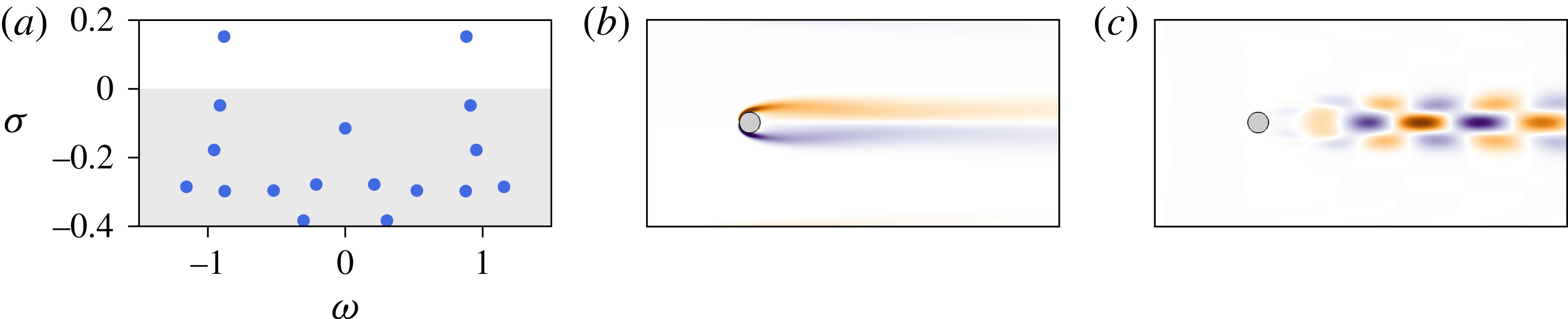
Reference Åkervik, Brandt, Henningson, Hœpffner, Marxen and Schlatter2006), is shown in figure 1(b). Figure 1(a,c) also provides the eigenspectrum of the linearized Navier–Stokes operator and the vorticity field associated with the leading unstable eigenmode for the sake of completeness. Though this eigenmode is clearly related to vortex shedding, it is well known that both its spatial distribution and the frequency of the associated eigenvalue differ quite significantly from that of the nonlinearly saturated von Kármán vortex street (Barkley Reference Barkley2006).
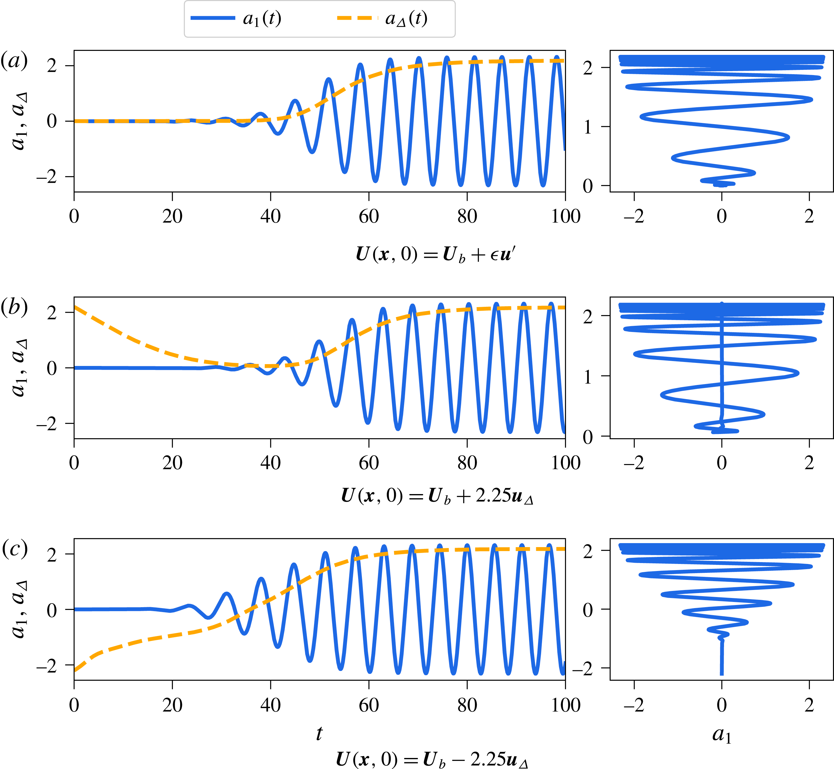
In the rest of this work, three different transient evolutions are considered. The first one, shown in figure 3(a), is started with the initial condition
 $$\begin{eqnarray}\boldsymbol{U}(\boldsymbol{x},0)=\boldsymbol{U}_{b}(\boldsymbol{x})+\unicode[STIX]{x1D716}\boldsymbol{u}^{\prime }(\boldsymbol{x}),\end{eqnarray}$$
where
 $\boldsymbol{U}_{b}$
is the linearly unstable base flow,
 $\boldsymbol{u}^{\prime }$
is the leading unstable eigenmode normalized such that it is unit norm and
 $\unicode[STIX]{x1D716}=10^{-6}$
. A direct numerical simulation has been run until a statistical steady state has been achieved. The dynamics of the system on the final attractor is then equidistantly sampled using
 $M=1000$
velocity field snapshots with a sampling frequency approximately 30 times larger than the vortex shedding frequency (Noack et al.
Reference Noack, Stankiewicz, Morzynski and Schmid2016). The shift mode, denoted
 $\boldsymbol{u}_{\unicode[STIX]{x1D6E5}}$
and depicted in figure 2(a), quantifies the distortion between the unstable base flow equilibrium and the mean flow. It has been shown to be crucially important for POD-based reduced-order modelling (Noack et al.
Reference Noack, Afanasiev, Morzynski, Tadmor and Thiele2003; Tadmor et al.
Reference Tadmor, Lehmann, Noack and Morzyński2010). The snapshot POD method of Sirovich (Reference Sirovich1987) has then been used to extract the two most energetic modes
 $\boldsymbol{u}_{1}$
and
 $\boldsymbol{u}_{2}$
, depicted in figures 2(b) and 2(c), respectively. The evolution in time of the POD coefficients is shown in figure 3(a), along with a projection of the system’s trajectory onto the (
 $a_{1}$
,
 $a_{\unicode[STIX]{x1D6E5}}$
) plane, where
 $a_{1}(t)$
is the amplitude of the POD mode
 $\boldsymbol{u}_{1}$
and
 $a_{\unicode[STIX]{x1D6E5}}(t)$
is the amplitude of the shift mode
 $\boldsymbol{u}_{\unicode[STIX]{x1D6E5}}$
. As shown in Noack et al. (Reference Noack, Afanasiev, Morzynski, Tadmor and Thiele2003), the system evolves on a low-dimensional paraboloid manifold characterized by
 $a_{\unicode[STIX]{x1D6E5}}\propto a_{1}^{2}+a_{2}^{2}$
.
Two additional transient evolutions, started with the initial conditions
 $$\begin{eqnarray}\boldsymbol{U}(\boldsymbol{x},t)=\boldsymbol{U}_{b}\pm 2.25\boldsymbol{u}_{\unicode[STIX]{x1D6E5}},\end{eqnarray}$$
are considered in order to capture the off-manifold dynamics. The first one, shown in figure 3(b), corresponds to a direct numerical simulation started from the mean flow. The second one, shown in figure 3(c), is characterized by an initial condition having a reversed flow region longer than that of the linearly unstable base flow. In both cases, the flow is rapidly attracted toward the vicinity of the fixed point before escaping away from it due to its linearly unstable nature. Including this off-manifold dynamics was deemed necessary in order to identify a physically consistent equation governing the dynamics of the mean-flow distortion
 $a_{\unicode[STIX]{x1D6E5}}(t)$
. In the rest, the transient evolutions shown in figure 3(a,b) are forming the training dataset used for the identification. The remaining transient evolution (see figure 3
c) is used for cross-validation purposes.
(a) Eigenspectrum of the linearized Navier–Stokes operator for the two-dimensional cylinder flow at
 $Re=100$
. Vorticity fields of (b) the base flow and (c) the leading linearly unstable eigenmode.

Vorticity fields of (a) the shift mode, (b) the first and (c) second POD modes of the cylinder flow at
 $Re=100$
.

Time evolution of the POD coefficients and corresponding trajectory in the phase space projected onto the (
 $a_{1}$
,
 $a_{\unicode[STIX]{x1D6E5}}$
) plane for the cylinder flow at
 $Re=100$
. The time evolution of
 $a_{2}(t)$
, not shown, is very similar to that of
 $a_{1}(t)$
. All three datasets used in the present work are presented.

4.2 Shear-driven cavity flow
The second flow configuration investigated is the incompressible shear-driven cavity flow. It is a geometrically induced separated boundary layer flow having a number of applications in aeronautics. The leading two-dimensional instability of the flow is mostly localized along the shear layer developing at the interface between the outer boundary layer flow and the inner-cavity flow (Sipp et al. Reference Sipp, Marquet, Meliga and Barbagallo2010). This oscillatory global instability of the external shear layer relies on two essential mechanisms. On the one hand, the convectively unstable nature of the shear layer causes perturbations to grow as they are convected downstream. On the other hand, the inner-cavity recirculating flow and the instantaneous pressure feedback provide the mechanisms allowing these same perturbations to eventually re-excite the upstream shear layer. The coupling between these mechanisms gives rise to a linearly unstable feedback loop at sufficiently high Reynolds numbers. In this case, the overall saturation process of the instability is well described by the second-order self-consistent model recently proposed by Meliga (Reference Meliga2017). Note that for compressible shear-driven cavity flows, a similar unstable feedback loop exists wherein the feedback mechanism is provided by upstream-propagating acoustic waves (Rossiter Reference Rossiter1964; Rowley, Colonius & Basu Reference Rowley, Colonius and Basu2002; Yamouni, Sipp & Jacquin Reference Yamouni, Sipp and Jacquin2013). This strictly two-dimensional linearly unstable flow configuration has served multiple purposes over the past decade: illustration of optimal control and reduced-order modelling (Barbagallo, Sipp & Schmid Reference Barbagallo, Sipp and Schmid2009), investigation of the nonlinear saturation process of globally unstable flows (Sipp & Lebedev Reference Sipp and Lebedev2007; Meliga Reference Meliga2017) or as an introduction to dynamic mode decomposition (Schmid Reference Schmid2010), to name just a few.
The computational domain and boundary conditions considered are the same as in Sipp & Lebedev (Reference Sipp and Lebedev2007). The Reynolds number is set to
 $Re=4250$
, based on the free-stream velocity
 $U_{\infty }$
and the depth
 $L$
of the open cavity. As for the cylinder, the linearly unstable flow, the corresponding eigenspectrum and the vorticity field of the leading unstable eigenmode are presented in figure 4 for the sake of completeness.
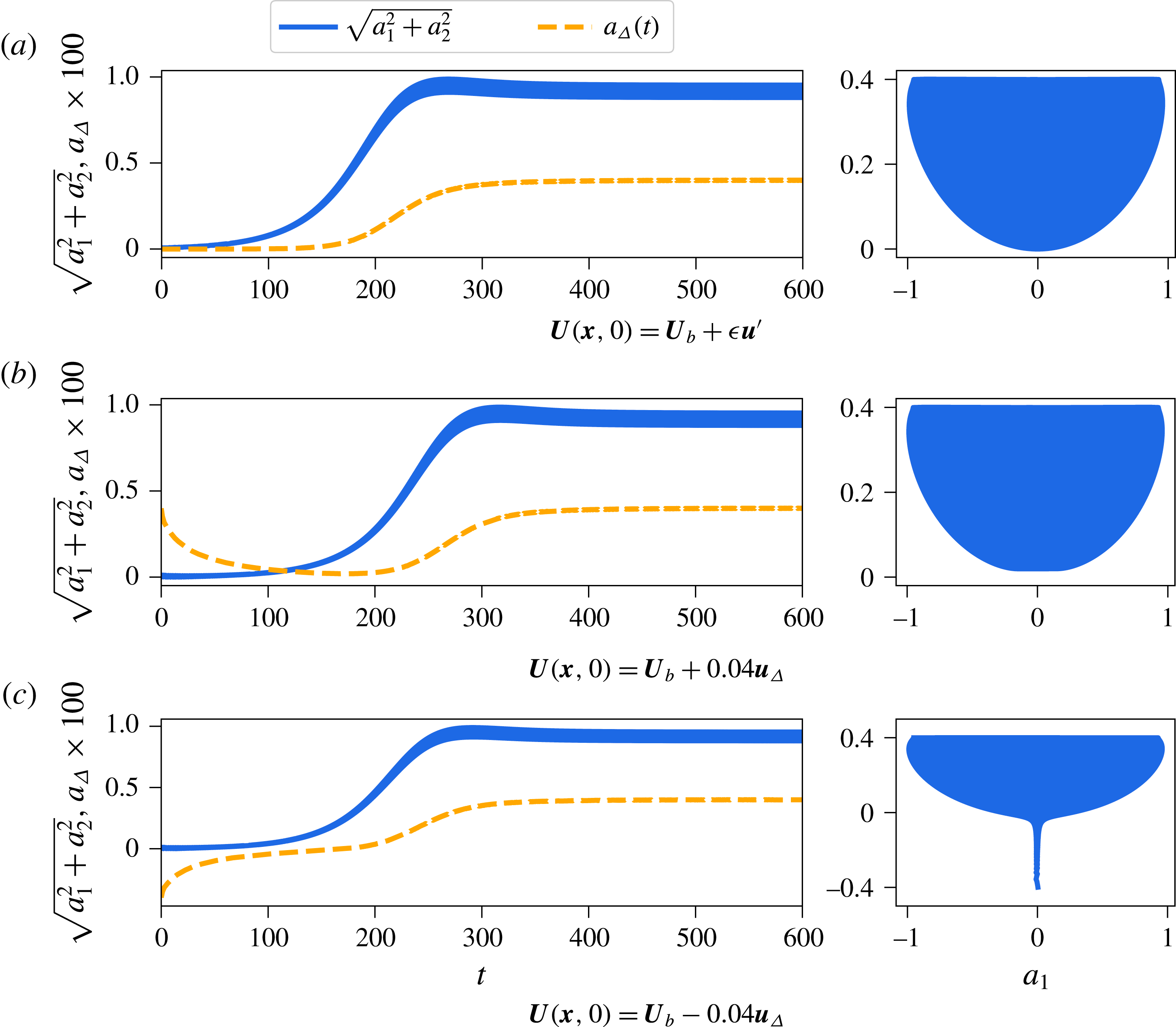
Three different transients are once again considered. The first one, shown in figure 6(a), is started with the initial condition
 $$\begin{eqnarray}\boldsymbol{U}(\boldsymbol{x},0)=\boldsymbol{U}_{b}(\boldsymbol{x})+\unicode[STIX]{x1D716}\boldsymbol{u}^{\prime }(\boldsymbol{x}),\end{eqnarray}$$
where
 $\boldsymbol{U}_{b}$
is the linearly unstable base flow,
 $\boldsymbol{u}^{\prime }$
is the leading unstable eigenmode normalized such that it is unit norm and
 $\unicode[STIX]{x1D716}=10^{-8}$
. This direct numerical simulation has been run until a statistically steady state has been reached. As for the cylinder flow, the dynamics of the attractor has been equidistantly sampled using
 $M=1000$
velocity field snapshots with a sampling frequency approximately 30 times larger than the oscillation frequency of the shear layer. The shift mode
 $\boldsymbol{u}_{\unicode[STIX]{x1D6E5}}$
is depicted in figure 5(a) and the leading POD mode is shown in figure 5(b). While the leading unstable eigenmode and the dominant POD mode of the cylinder flow are extremely different, this is not the case for the shear-driven cavity flow at
 $Re=4250$
. Note furthermore that, despite the fundamental difference of the geometry, the different frequency of the oscillations and the smaller growth rate of the instability, the two flows considered herein appear to exhibit relatively similar dynamics when looking at the systems’ trajectories projected onto the
 $a_{1}$
–
 $a_{\unicode[STIX]{x1D6E5}}$
planes: both low-dimensional representations of the flows appear to evolve along a parabolic manifold; see figures 3(b) and 6(b). As for the cylinder, two additional transients, started from either side of the fixed point in the direction of the shift mode, have been included. Once again, the transients shown in figure 6(a,b) are forming the training dataset used for the identification problem, while the transient depicted in figure 6(c) will be used for cross-validation purposes only.
(a) Eigenspectrum of the linearized Navier–Stokes operator for the shear-driven cavity flow at
 $Re=4250$
. Vorticity fields of (b) the base flow and (c) the leading linearly unstable eigenmode. The dashed lines indicate the spatial extent over which the free-slip boundary condition is imposed.

Vorticity fields of (a) the shift mode and (b) the first POD mode for the shear-driven cavity flow at
 $Re=4250$
.

Time evolution of the POD coefficients and corresponding trajectory in the phase space projected onto the
 $(a_{1},a_{2})$
plane for the shear-driven cavity flow at
 $Re=4250$
. The time evolution of
 $a_{2}(t)$
, not shown, is very similar to that of
 $a_{1}(t)$
. All three datasets used in the present work are presented.

5 Results and discussion
Following the seminal work of Noack et al. (Reference Noack, Afanasiev, Morzynski, Tadmor and Thiele2003), so-called quadratic Galerkin regression models are constructed from the basic building blocks necessary for reduced-order modelling of the flow configurations considered, i.e. a linear operator
 ${\mathcal{L}}$
and an energy-preserving quadratic nonlinearity
 ${\mathcal{N}}(\boldsymbol{a})$
. For that purpose, the library
 $\unicode[STIX]{x1D723}(\boldsymbol{a})$
used in the identification process is defined as
 $\left[\begin{array}{@{}cc@{}}P_{1}(\boldsymbol{a}) & P_{2}(\boldsymbol{a})\end{array}\right]$
, i.e. all the polynomials of degree 2 or less in the entries of
 $\boldsymbol{a}$
. A second type of models, cubic Galerkin regression models, are made of the same basic building blocks as their quadratic counterparts. They moreover include higher-order nonlinearities which can serve to model the truncated modes, as discussed in § 3.2. For that purpose, the library
 $\unicode[STIX]{x1D723}(\boldsymbol{a})$
used in the identification process is defined as
 $\left[\begin{array}{@{}ccc@{}}P_{1}(\boldsymbol{a}) & P_{2}(\boldsymbol{a}) & P_{3}(\boldsymbol{a})\end{array}\right]$
, i.e. all the polynomials of degree 3 or less in the entries of
 $\boldsymbol{a}$
. Up to 57 coefficients then need to be identified for the present case with
 $n=3$
state variables.
5.1 Cylinder flow
Figures 8 and 9 provide a comparison of the dynamics predicted by the low-dimensional Galerkin regression models identified using constrained sparse regression against the dynamics of the original system for the two-dimensional cylinder flow at
 $Re=100$
. It also provides the dynamics predicted by two additional data-driven reduced-order models, namely:
-
(i) the minimal Galerkin projection model including only the shift mode and the first two POD modes,
-
(ii) a Galerkin projection model including the shift mode and the first eight POD modes.
5.1.1 Model selection
Model selection and cross-validation are crucial components of system identification. The goal is to identify, among all candidate models, the parsimonious model that optimally balances model accuracy and model complexity. As the sparsifying parameter
 $\unicode[STIX]{x1D706}$
is varied in the SINDy procedure, a Pareto front is swept out, reducing the combinatorially many candidate models down to a small handful of candidates models. Mangan et al. (Reference Mangan, Kutz, Brunton and Proctor2017) have recently demonstrated how SINDy can be combined with the well-known Akaike information criterion (AIC) (Akaike Reference Akaike1974) or the Bayes information criterion (BIC) (Schwarz et al.
Reference Schwarz1978) in order to select the most parsimonious model from this Pareto front. Given a candidate model, the associated AIC score is given by
 $$\begin{eqnarray}\text{AIC}=2k-2\ln (L(\boldsymbol{a},\unicode[STIX]{x1D729}))+2\frac{(k+1)(k+2)}{(m-k-2)},\end{eqnarray}$$
where
 $L(\boldsymbol{a},\unicode[STIX]{x1D729})$
is the loss function of the observations
 $\boldsymbol{a}$
given the best-fit parameter values
 $\unicode[STIX]{x1D729}$
of the candidate model and
 $k$
is the total number of free parameters. The last term in (5.1) is a finite sample size correction where
 $m$
is the total number of observations used to cross-validate the model. These training and testing datasets are the same as those shown in figure 3. For two models of the same accuracy, the AIC score will penalize the one having the larger number of terms.
The AIC scores for each candidate model can have a wide range of values, hence requiring a rescaling by the minimum AIC value. The relative AIC score is thus given by
 $$\begin{eqnarray}\unicode[STIX]{x1D6E5}=\text{AIC}-\text{AIC}_{min}.\end{eqnarray}$$
The different candidate models can then be ranked based on this relative AIC score. Following Mangan et al. (Reference Mangan, Kutz, Brunton and Proctor2017), models with
 $\unicode[STIX]{x1D6E5}\leqslant 2$
have so-called strong support, models with
 $4\leqslant \unicode[STIX]{x1D6E5}\leqslant 7$
have weak support and models with
 $\unicode[STIX]{x1D6E5}\geqslant 10$
have no support. It should be emphasized that the model characterized by
 $\unicode[STIX]{x1D6E5}=0$
is not necessarily the best model possible, but only the best one among the different models tested.
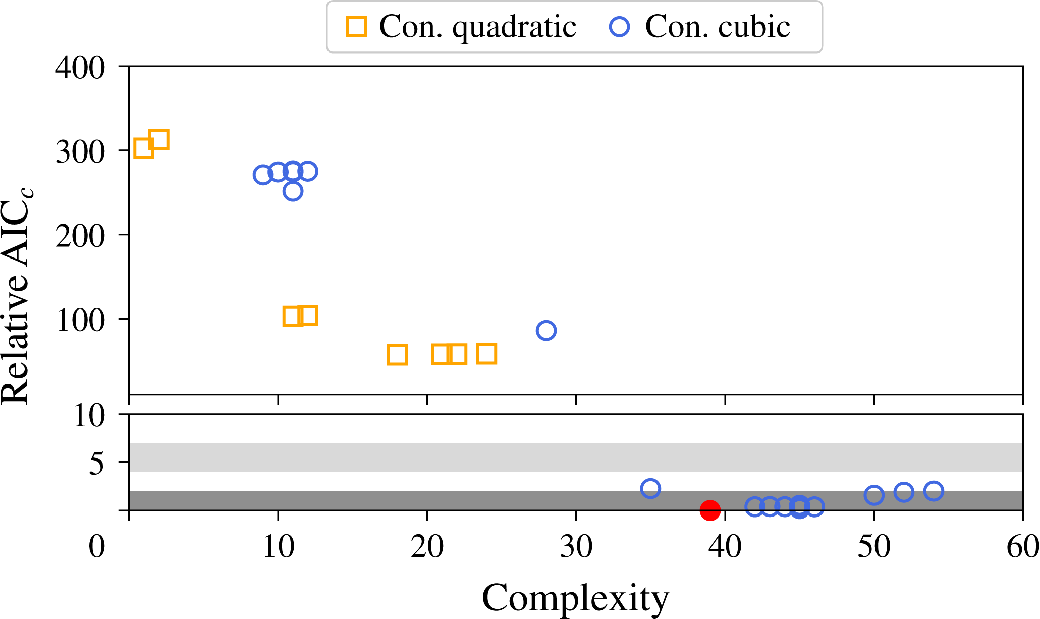
Figure 7 depicts the distribution of all the different models identified in the complexity versus AIC
 $_{\text{c}}$
plane for the two-dimensional cylinder flow at
 $Re=100$
. Note that none of the unconstrained models are shown as they have all diverged in the cross-validation stage when trying to reproduce the dynamics of the transient evolution shown in figure 3(c). This observation will be investigated in § 5.1.3. Although the quadratic Galerkin regression models have lower complexity and appear at first to be more physical, it is interesting to note that they are largely dominated by the cubic models. In the rest of this section, only the best constrained quadratic model and the best constrained cubic model are considered. Excluding the transient evolution shown in figure 3(c) from the validation stage, a similar analysis is performed in order to select the unconstrained models considered in the following sections.
Distribution of all the different constrained low-order models identified in the complexity versus AIC
 $_{c}$
plane. The red circle corresponds to the best model identified.

5.1.2 Qualitative comparisons
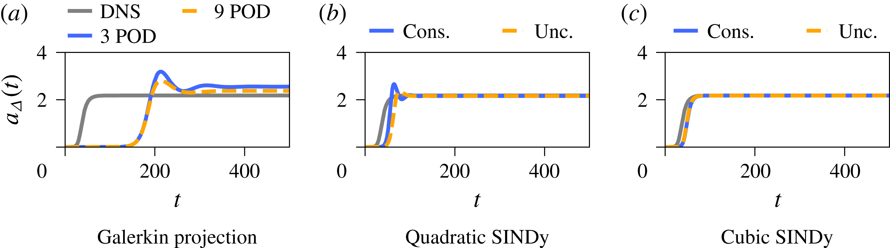
Let us consider the first transient evolution forming our training dataset, shown in figure 3(a). Figures 8 and 9 provide visual comparisons of the dynamics predicted by the different models. The time evolution of the mean-flow distortion predicted by the low-dimensional Galerkin projected systems, shown in figure 8(a), indicates that the duration of the transients is largely over-estimated and that an energy overshoot occurs once nonlinear saturation kicks in. On the one hand, the over-estimation of the duration of transients results from the fact that the leading POD modes (see figure 2) provide only a crude approximation of the leading linear instability eigenmodes (see figure 1). On the other hand, the overshoot and the ensuing larger amplitude of the mean-flow distortion mostly result from the disruption of the energy cascade due to neglecting the higher-harmonic POD modes. Being entirely neglected, these higher harmonics cannot absorb the excess energy produced by the two most energetic modes. The latter then grow beyond the correct value until the mean-flow distortion
 $a_{\unicode[STIX]{x1D6E5}}(t)$
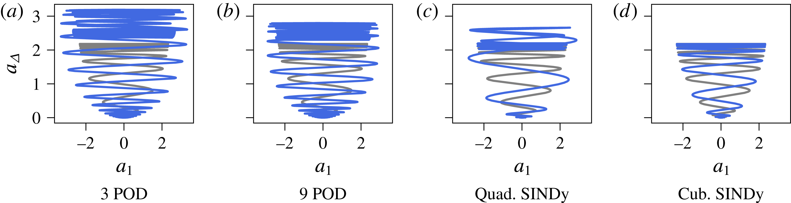
can eventually absorb this excess energy via the coupling terms. As shown in figure 8(b), the constrained and unconstrained quadratic Galerkin regression models suffer from similar drawbacks, although the duration of transients is shortened and the final amplitude of the mean-flow distortion is in agreement with that of the original system. Moreover, the unconstrained model a priori performs better than the constrained one. Comparatively, the cubic Galerkin regression models provide an almost perfect fit to the original data, as shown in figures 8(b) and 9(d): the amplitude of the limit cycle is less than 0.5 % higher than that of the original system while the saturation of the mean-flow distortion differs by less than 0.1 %. Moreover, the inclusion of the cubic nonlinearities, modelling the influence of the truncated modes, has a stabilizing effect, hence preventing the energy overshoot and larger limit cycle amplitude observed for the quadratic models.
Comparison of the time evolution of the mean-flow distortion
 $a_{\unicode[STIX]{x1D6E5}}$
predicted by the different data-driven models for the two-dimensional cylinder flow at
 $Re=100$
. The transient evolution considered, which is part of the training dataset, is the one depicted in figure 3(a).

Comparison of the trajectory in the
 $a_{1}{-}a_{\unicode[STIX]{x1D6E5}}$
plane predicted by the different reduced-order models for the two-dimensional cylinder flow at
 $Re=100$
. The light grey trajectory is the one given by a direct numerical simulation. Only the constrained cases are reported for the Galerkin regression models.

5.1.3 Quantitative analysis
Table 1 reports the growth rate and circular frequency of the leading eigenvalue of the low-dimensional linear operator
 ${\mathcal{L}}$
for the different models considered and compares it against the values obtained from a linear stability analysis of the linearized Navier–Stokes equations. As discussed previously, the leading POD modes (see figure 2) provide only a crude approximation of the leading linear instability eigenmodes (see figure 1). As a result of this crude approximation, the growth rate of the leading eigenvalue of the low-dimensional operator
 ${\mathcal{L}}$
obtained by Galerkin projection is three to four times smaller than the actual value obtained by linear stability analysis, hence explaining the over-estimation of the transients duration, while the associated frequency is 10 % larger than the actual one. Similarly, the growth rate of the unconstrained and constrained quadratic models are 30 % smaller than the correct value. Compared to these models, the spectral properties of the cubic Galerkin regression models are in excellent agreement with the results obtained from linear stability analysis of the Navier–Stokes equations, the identified growth rate
 $\unicode[STIX]{x1D70E}$
being only 6 % larger than the true one while the corresponding frequency is only up to 1 % different than the correct value. Introducing higher-order nonlinearities in the model identification thus not only allows us to take into account the influence of the truncated modes on the driving ones, but it also enables the optimization procedure to correctly estimate the growth rate of the linear instability.
Comparison of growth rate
 $\unicode[STIX]{x1D70E}$
and circular frequency
 $\unicode[STIX]{x1D714}$
of the leading eigenvalue for the different models considered. Results from a global stability analysis of the Navier–Stokes (N–S) equations are also reported. The last row also reports the value of the decay rate
 $\unicode[STIX]{x1D70E}_{\unicode[STIX]{x1D6E5}}$
associated with the shift mode. Note that only the first two transients shown in figure 3 are part of the training dataset.

Now focusing our attention on the decay rate
 $\unicode[STIX]{x1D70E}_{\unicode[STIX]{x1D6E5}}$
of the shift mode, it can be seen that both constrained models identify the mean-flow distortion as being linearly stable, so does the unconstrained cubic model. Although the unconstrained quadratic model appears to outperform the constrained one when looking at the evolution depicted in figure 8(b), it can be seen from table 1 that it surprisingly identifies the mean-flow distortion as being linearly unstable. This misprediction of the linearly stable nature of the mean-flow distortion also explains why the present unconstrained model fails to reproduce the dynamics of the third transient evolution (see figure 3
c) used in the cross-validation stage. If one were to consider only our first two transient evolutions (figure 3
a,b) without prior knowledge of the problem, one could easily conclude that the system is indeed linearly unstable in the
 $a_{\unicode[STIX]{x1D6E5}}$
direction. From an identification point of view, the governing equations for
 $a_{1}$
,
 $a_{2}$
and
 $a_{\unicode[STIX]{x1D6E5}}$
are obtained independently from one another in the absence of constraints that would otherwise couple them. As a consequence, an equation predicting a linear instability of
 $a_{\unicode[STIX]{x1D6E5}}$
is thus the simplest model identifiable which balances parsimony and consistency with measurements available in our training dataset. Such a model is however not acceptable as it could lead to a misunderstanding of the physics at play. This example thus clearly demonstrates the benefits of introducing physics into the identification process: coupling all of the equations governing the evolution of the system through the use of constraints mimicking the energy-preserving nature of the quadratic nonlinearity enables the identification of a much more physical low-dimensional system.
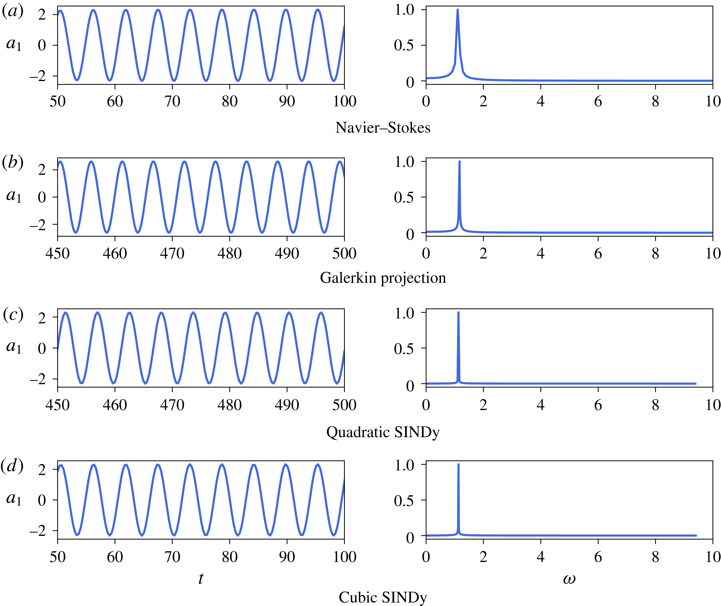
Finally, figure 10 depicts time series of
 $a_{1}(t)$
in the nonlinearly saturated stage and the associated Fourier spectrum for the different models considered. Comparing these different Fourier spectra, it is clear that the vortex shedding frequency
 $\unicode[STIX]{x1D714}=1.15$
(
 $St=0.18$
) predicted by all the models in the nonlinear regime is in excellent agreement with that observed from direct numerical simulation.
Time series of the nonlinearly saturated dynamics of
 $a_{1}(t)$
and normalized Fourier spectra for the different models considered for the two-dimensional cylinder flow at
 $Re=100$
. Note that the larger width of the peak in (a) is solely related to the smaller integration window used in direct numerical simulation. Only the constrained cases are reported for the Galerkin regression models.

5.2 Shear-driven cavity flow
Figure 11 provides a comparison of the dynamics predicted by the low-dimensional Galerkin Regression models identified using constrained sparse regression against the dynamics of the original system for the two-dimensional shear-driven cavity flow at
 $Re=4250$
. It also provides the dynamics predicted by two additional data-driven reduced-order models, namely:
-
(i) the minimal Galerkin projection model including only the shift mode and the first two POD modes,
-
(ii) a Galerkin projection model including the shift mode and the first six POD modes.
The model selection procedure, being the same as described in § 5.1, is thus not discussed again for the present case.
5.2.1 Overview
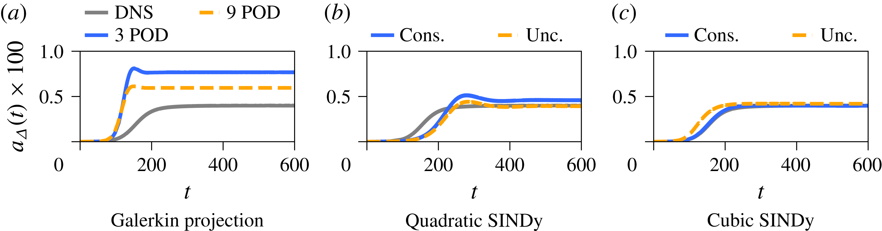
Figure 11 provides visual comparisons of the dynamics predicted by the different models for the two-dimensional shear-driven cavity flow at
 $Re=4250$
. Although the geometry and the physics are quite different from that of the two-dimensional cylinder flow, the present Galerkin projection models suffer from similar drawbacks as before: a misprediction of the transients duration and the saturation to higher mean-flow distortion due to the disruption of the energy cascade. However, the key difference is that for the shear-driven cavity flow, the growth rate of the linear instability mode is slightly over-predicted by the Galerkin projection models. Looking now at figure 11(b), the two quadratic Galerkin regression models correctly reproduce the asymptotic dynamics of the shear-driven cavity flow. Both of them slightly over-predict the duration of the transients. Finally, both cubic models appear to exhibit similar accuracy as shown in figure 11(c), although the unconstrained version appears to saturate slightly faster.
Comparison of the time evolution of the mean-flow distortion
 $a_{\unicode[STIX]{x1D6E5}}$
predicted by the different data-driven models for the two-dimensional shear-driven cavity flow at
 $Re=4250$
.

5.2.2 Quantitative analysis
Table 2 provides a comparison of the growth rate
 $\unicode[STIX]{x1D70E}$
and circular frequency
 $\unicode[STIX]{x1D714}$
of the leading unstable eigenvalue for each of the models considered. As assessed from figure 11, all of these growth rates are in qualitative agreement with that obtained from a global linear stability analysis of the Navier–Stokes equations, the constrained cubic model differing by less than 1 %. One way to further improve the accuracy of the quadratic models would be to constrain the eigenspectrum of the low-dimensional linear operator to be a subset of its high-dimensional counterpart. Such a constraint on the determinant of the low-dimensional linear operator is however a non-convex constraint and does not fall within the scope of the library CVXOPT used in the present work.
Let us finally explore the decay rate
 $\unicode[STIX]{x1D70E}_{\unicode[STIX]{x1D6E5}}$
of the shift mode predicted by the different models, shown in table 2. Contrary to the cylinder flow, all models presented here correctly identify a linearly stable shift mode. Note however that if only the transient shown in figure 6(a) had been considered, the unconstrained quadratic model would suffer from the same shortcoming as for the cylinder flow (i.e. linearly unstable shift mode). Given that the relative distance to the critical Reynolds number is comparatively smaller in the present case compared to the cylinder flow, the influence of the truncated modes is expected to be less important. One might thus hypothesize that the correctness of the unconstrained quadratic model is related to this fact. In any case, this example once again underlines the importance of using physics-based constraints in order to identify physically relevant low-order models.
Comparison of growth rate
 $\unicode[STIX]{x1D70E}$
and circular frequency
 $\unicode[STIX]{x1D714}$
of the leading eigenvalue for the different models considered. Results from a global stability analysis of the Navier–Stokes equations are also reported. The last row also reports the value of the decay rate
 $\unicode[STIX]{x1D70E}_{\unicode[STIX]{x1D6E5}}$
associated with the shift mode.

6 Conclusion
This paper develops a new data-driven Galerkin regression framework to identify nonlinear reduced-order models of a fluid. The resulting models incorporate a number of beneficial features of standard Galerkin projection, making them easy to interpret and use, but without the need for access to a high-fidelity Navier–Stokes model for the projection. Galerkin regression models also provide a more flexible model identification, in that they readily generalize to include higher-order nonlinear terms that model the effect of truncated modes; the inclusion of these terms is shown to be extremely effective in the examples presented here. In fact, including higher-order nonlinear terms in the models prevents underfitting, and allows for models with improved accuracy in terms of fewer, more energetic modes. The Galerkin regression framework leverages the recent sparse identification of nonlinear dynamics (SINDy) algorithm (Brunton et al. Reference Brunton, Proctor and Kutz2016a ), and generalizes it to include user-provided constraints directly into the sparsity-promoting regression. These additional constraints can be used to enforce a priori known values of some of the regression coefficients, inherent symmetries of the system of equations or some physical behaviour such as the energy-preserving nature of the quadratic nonlinearity of the Navier–Stokes equations.
The two-dimensional cylinder flow and the shear-driven cavity have each been carefully analysed to illustrate the system identification capabilities of the resulting algorithm. For that purpose, two polynomial libraries have been used and the constraints have been chosen in order to enforce different physical properties. The accuracy and performance of the so-called Galerkin regression models have been compared against reduced-order models derived using a classical Galerkin projection method. All of the regression models qualitatively reproduce the main features of the original system: linear instability of the fixed point and final saturation to a periodic limit cycle. Though these models rely essentially on a data-driven approach, visual inspection of their trajectories in the phase space highlights the connection between the quadratic models and the models obtained using a Galerkin projection procedure in the seminal work of Noack et al. (Reference Noack, Afanasiev, Morzynski, Tadmor and Thiele2003). Moreover, both flow configurations highlight the importance of including cubic nonlinearities into the admissible pool of functions for the identification process, something utterly impossible with classical Galerkin projection without significant additional post-analysis. These cubic terms then model the influence of the truncated modes onto the driving ones, eventually enabling the identification of a low-dimensional system with much better predictive capabilities. Although some of the unconstrained models identified reproduce faithfully the dynamics of the original system, analysis of their spectral properties has highlighted the importance of incorporating physically meaningful constraints into the regression to ensure that the identified model has the correct physical behaviour. In their absence, the SINDy algorithm can incorrectly identify the mean flow distortion as a linearly unstable manifold of the fixed point, while adding constraints results in the correct identification of a linearly stable eigenvalue.
Despite its promise, such an approach to system identification still suffers from certain limitations. One such limitation is illustrated by the quadratic constrained models which tend to under-estimate the growth rate of the linear instability. Given prior knowledge of the linear stability of the high-dimensional system (see § 4.2), one could then constrain the eigenspectrum of the low-dimensional linear operator to be a subset of its high-dimensional counterpart. Such a constraint, involving the determinant of the low-dimensional matrix, falls outside the scope of convex optimization. Current developments, based on the nonlinear optimization library NLOPT (Johnson Reference Johnson2014), attempt to overcome such limitations. One might also argue that the systems considered in the present work are inherently low-dimensional and are thus not representative of the high-dimensionality of a transitional or turbulent flow. However, such flows have already been modelled with some success using a Galerkin projection procedure (Gloerfelt Reference Gloerfelt2008). Given the parallels drawn in the present work between Galerkin projection and Galerkin regression, there is reason to believe that the present approach may be successfully applied to such flows as well. Indeed, this is an exciting future direction and is the subject of ongoing work. Including high-order nonlinear terms in the pool of admissible functions in combination with the sparsity-promoting capabilities of the algorithm might furthermore allow the identification of smaller and more robust reduced-order models without significantly altering their accuracy and predictive capabilities.
Extending these constrained regression methods to experimental data may also present unique challenges and rewards. Many numerical schemes are designed to preserve energy; however, in turbulent simulations and experiments where sensors have limited bandwidth, dissipation may be large enough to affect the stability of models. Explicitly incorporating energy-preserving constraints in the SINDy regression may be especially important in these problems to find nearby conservative systems.
Acknowledgements
We are grateful for many fruitful discussions with B. Noack, J. Proctor and N. Kutz. We also appreciate valuable feedback from S. Dawson and C. Rowley. S.L.B. acknowledges generous funding support from the US Defense Advanced Research Projects Agency (DARPA HR0011-16-C-0016) and from the US Air Force Office of Scientific Research (AFOSR FA9550-16-1-0650 and FA9550-18-1-0200).
Appendix A. Connection with NARMAX
Over the years, a number of different approaches have been proposed for the identification of nonlinear dynamical systems from measured data. One of the most versatile and popular approach is NARMAX (Billings Reference Billings2013): nonlinear auto-regressive model with exogeneous inputs. Although it targets the identification of discrete-time dynamical systems, its formulation is very close to that of the SINDy framework. Apart from the discrete-time versus continuous-time representations of the dynamics, one core difference between these two approaches essentially lies in the algorithm used to enforce the parsimony of the model: NARMAX classically uses the orthogonal least-squares procedure, while SINDy is based on a
 $\ell _{1}$
-penalized or iterative hard-thresholded least-squares regression. In addition, the SINDy framework has been extended significantly, including to identify partial differential equations, to connect with Koopman operator theory, and to incorporate information criteria, rational function nonlinearities, and, in the present work, constraints. However, SINDy may be considered as a close relative of the NARMAX family of system identification, and the constrained SINDy algorithm may be used to identify effective NARMAX models, as demonstrated in this Appendix A.
Here, we apply SINDy to identify NARMAX-like models of the two-dimensional cylinder flow at
 $Re=100$
; we only consider this flow configuration for simplicity. As before, the first two transient evolutions depicted in figure 3(a,b) form the training dataset, while the last trajectory (see figure 3
c) is used solely for cross-validation purposes. In the rest, we postulate that the discrete-time model can be written as
 $$\begin{eqnarray}\boldsymbol{a}(t)={\mathcal{L}}\boldsymbol{a}(t-\unicode[STIX]{x1D70F})+{\mathcal{N}}(\boldsymbol{a}(t-\unicode[STIX]{x1D70F})).\end{eqnarray}$$
Given a library of admissible right-hand side functions
 $\unicode[STIX]{x1D723}(\boldsymbol{a})$
, this discrete-time system can be recast as
 $$\begin{eqnarray}\boldsymbol{a}(t)=\unicode[STIX]{x1D723}(\boldsymbol{a}(t-\unicode[STIX]{x1D70F}))\unicode[STIX]{x1D729}.\end{eqnarray}$$
As before,
 $\unicode[STIX]{x1D729}_{i}$
is a sparse column vector indicating which functions from the library
 $\unicode[STIX]{x1D723}(\boldsymbol{a})$
are active in the equation governing the dynamics of
 $a_{i}(t)$
. Given time-series data of
 $\boldsymbol{a}(t)$
, these sparse column vectors can once again be identified using the SINDy algorithm, based on a
 $\ell _{1}$
-regularized least-squares minimization. The last parameter which has to be set before the identification is the time lag
 $\unicode[STIX]{x1D70F}$
. Here, it is chosen as
 $\unicode[STIX]{x1D70F}=0.25$
.
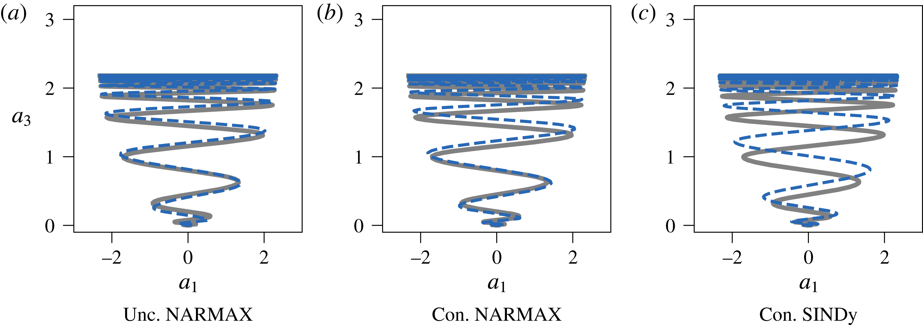
Figure 12 depicts the trajectory in the (
 $a_{1}$
,
 $a_{3}$
) plane predicted by an unconstrained NARMAX-like model, a constrained one and the constrained cubic Galerkin regression model presented earlier. Although all three trajectories are virtually identical, it must be noted that the two constrained models are more parsimonious than the unconstrained one. Indeed, while the unconstrained NARMAX model has 45 terms in its right-hand side, the constrained NARMAX and Galerkin regression models have 35 and 37 terms, respectively. Moreover, the unconstrained model fails to reproduce the transient evolution shown in figure 3(c). Importantly, both NARMAX models are identified using the SINDy algorithm and code base. This example clearly underlines the versatility of the SINDy framework and the benefit of introducing physics into the identification process by means of constraints.
Comparison of the trajectory in the
 $a_{1}{-}a_{\unicode[STIX]{x1D6E5}}$
plane predicted by the different reduced-order models for the two-dimensional cylinder flow at
 $Re=100$
. The light grey trajectory is from direct numerical simulation.