4.1 Weighted estimator

The identification result in Theorem 1 expresses the T-CACE as a ratio of two terms: (1) the generalized ITT effect and (2) the generalized first stage. In this section, we construct a weighted estimator for by deriving separate weighted estimators for both the numerator and the denominator. We show that the weighted estimator is a consistent estimator of the T-CACE and derive its asymptotic distribution.

We begin by defining the following weights:

(3) $$ \begin{align} w_z(X) := \frac{{\mathbb{P}}(S = 0 {\,|\,} X)}{{\mathbb{P}}(S = 1 {\,|\,} X)} \cdot \frac{1}{\mathbb{P}(Z = z {\,|\,} S = 1, X)}, \end{align} $$

where $\mathbb {P}(S=0|X)/{\mathbb {P}(S=1|X)}$ accounts for distribution shifts in the observed covariates between the study sample and the target population, and $\mathbb {P}(Z=z|S=1, X)$ accounts for imbalance in the treatment and control groups. In the context of an RCT, the probability of treatment is known by the researcher. The weights in Equation (3) are equivalent to the standard generalization weights introduced in Cole and Stuart (Reference Cole and Stuart2010). A common approach to estimating the weights is to estimate a propensity score model for the underlying sample selection process. Alternatively, researchers can employ balancing approaches, which directly target the distributional differences in the underlying covariates without directly fitting a parametric model (e.g., Hainmueller Reference Hainmueller2012; Imai and Ratkovic Reference Imai and Ratkovic2014).

We define the re-weighted ITT effect as

(4) $$ \begin{align} \widehat{\tau}_{w}^{Y} = \frac{\sum_{i:S_i=1} \widehat{w}_1(X_i) Z_i Y_i} {\sum_{i:S_i=1} \widehat{w}_1(X_i) Z_i} - \frac{\sum_{i:S_i=1} \widehat{w}_0(X_i) (1-Z_i)Y_i} {\sum_{i:S_i=1} \widehat{w}_0(X_i) (1-Z_i)}, \end{align} $$

where $\widehat w_1(X_i)$ and $\widehat w_0(X_i)$ are estimates of the true generalization weights in Equation (3). This is the standard weighted estimator used in the generalizability literature, which ignores noncompliance.

We also define the weighted estimator for the treatment received:

(5) $$ \begin{align} \widehat{\tau}_{w}^{D} = \frac{\sum_{i:S_i=1} \widehat{w}_1(X_i) Z_i D_i} {\sum_{i:S_i=1} \widehat{w}_1(X_i) Z_i} - \frac{ \sum_{i:S_i=1} \widehat{w}_0(X_i) (1-Z_i)D_i} {\sum_{i:S_i=1} \widehat{w}_0(X_i) (1-Z_i)}. \end{align} $$

$\widehat {\tau }_{w}^{D}$ is analogous to $\widehat {\tau }_{w}^{Y}$ in that both share the same weights to account for the distribution shift. However, $\widehat {\tau }_{w}^{D}$ pertains to treatment received rather than the outcome. Notably, $\widehat {\tau }_{w}^{D}$ effectively estimates the denominator of the identification result of Theorem 1.

The weighted estimator of is given by the ratio of these two quantities:

(6) $$ \begin{align} \widehat{\tau}_{w} = \frac{\widehat{\tau}_{w}^{Y}}{\widehat{\tau}_{w}^{D}}. \end{align} $$

If the estimated weights $\widehat w_1(X)$ and $\widehat w_0(X)$ are correctly specified, then the weighted estimator is a consistent estimator for .

Theorem 4.1 Consistency of the weighted estimator

Assume that $\mathbb {P}(S = 1) = \frac {n}{n+N}$ is fixed, so that the ratio between n and N remains constant as $n \to \infty $ and $N \to \infty $ . Assume $\sup _{x \in \mathcal {X}} \left |\widehat {w}_1(x) - w_1(x)\right | = o_p(1)$ and $\sup _{x \in \mathcal {X}} \left |\widehat {w}_0(x) - w_0(x)\right | = o_p(1).$ Then, under Assumptions 1–4,

The fixed ratio condition is used only as an asymptotic device and ensures that as the study sample grows toward infinity, the corresponding target population size also grows toward infinity. In settings when researchers are interested in finite-population settings, we refer readers to Li and Ding (Reference Li and Ding2017). To characterize the asymptotic distribution of the weighted estimator, we begin by first assuming that the selection model and the treatment assignment model are known. Then, the weighted estimator will be asymptotically normally distributed.

Theorem 4.2 Asymptotic distribution of the weighted estimator

Assume the selection model (i.e., $\mathbb {P}(S = 1 \,|\, X)$ ) and the treatment assignment model (i.e., $\mathbb {P}(Z = 1 \,|\, S=1, X)$ ) are both known. Let $g(\cdot ):\mathbb {R}^6\rightarrow \mathbb {R}$ be defined as $g(\theta ) = (\frac {\theta _1}{\theta _3} - \frac {\theta _2}{\theta _4})/(\frac {\theta _5}{\theta _3} - \frac {\theta _6}{\theta _4}).$ Denote $\nabla g$ as its gradient vector. Then, under the same assumptions as Theorem 2 and the regularity conditions $\mathbb {E} \left [w_z(X)^2 Y^2\right ] < \infty ,$

where we define the covariance matrix $\Sigma _{\theta ^*}$ in (C.8) of Section C.3 of the Supplementary Material.

The result of Theorem 3 follows from establishing the asymptotic normality of each component of $\widehat {\tau }_{w}$ by leveraging the theory of estimating equations. In particular, we write $\widehat {\tau }_{w}$ as the function g of an M-estimator (Huber Reference Huber1992) and then apply the Delta method to g. The covariance matrix, $\Sigma _{\theta ^*},$ though unknown, can be consistently estimated using its empirical counterpart (see Section D of the Supplementary Material for details).

In practice, researchers do not know the true probability of selecting into the study sample. In Section A of the Supplementary Material, we provide a similar result for settings in which the probability of selection is estimated. In practice, we can construct Wald-type confidence intervals for by replacing the covariance matrix in Theorem 3 with its empirical counterpart. The details of the construction of the empirical sandwich-type variance estimator and the Wald-type confidence intervals are given in Section D of the Supplementary Material.

4.2 Weighted least squares

While Section 4.1 introduces an estimator that allows us to consistently recover the T-CACE, a well-known drawback to weighted estimators is the potential efficiency loss that occurs from reweighting (Huang et al. Reference Huang, Egami, Hartman and Miratrix2023; Miratrix et al. Reference Miratrix, Sekhon, Theodoridis and Campos2018). This concern is exacerbated in the IV setting, where the combination of reweighting as well as a potentially weak instrument can result in large amounts of variance inflation (Hartman and Huang Reference Hartman and Huang2024). To combat some of the losses in efficiency, we propose a weighted least squares approach to estimating the T-CACE.

More formally, we define the covariate-adjusted weighted least squares estimator as

(7) $$ \begin{align} \widehat{\tau}_{\text{wls}} := \frac{\widehat{\tau}^{Y}_{\text{wls}}}{\widehat{\tau}^{D}_{\text{wls}}}, \end{align} $$

where $\widehat {\tau }^{Y}_{\text {wls}}$ and $\widehat {\tau }^{D}_{\text {wls}}$ are given by

(8) $$ \begin{align} & (\widehat{\tau}_{\text{wls}}^{Y}, \widehat{\gamma}^Y) := \mathop{\mathrm{arg\,min}}_{\tau, \gamma}\sum_{i:S_i=1}\widehat{w}(X_i) \left\{ Y_i - (\tau Z_i + \gamma^T X_i) \right\}^2, \nonumber\\ & (\widehat{\tau}_{\text{wls}}^{D}, \widehat{\gamma}^D) := \mathop{\mathrm{arg\,min}}_{\tau, \gamma}\sum_{i:S_i=1}\widehat{w}(X_i) \left\{ D_i - (\tau Z_i + \gamma^T X_i)\right\}^2. \end{align} $$

Intuitively, the weighted least squares estimator reweights the residual variance of the outcome and treatment received, after controlling for covariates X. If the pre-treatment covariates X are predictive of Y and $D,$ incorporating X into the model will reduce the weighted sample residual variance, leading to a more precise estimate. Furthermore, while the estimated weights depend on covariates that are measured across both the study sample and the target population, the regression uses only observations across the study sample. Using the weighted least squares approach allows researchers to leverage additional covariates, measured across just the study sample, to help improve efficiency.

We can view the standard weighted estimator $\widehat {\tau }_{w}$ as a special case of $\widehat {\tau }_{\text {wls}},$ in which no covariates X are included except for the intercept. We show in Theorem A.2 in the Supplementary Material that, under the same conditions as the weighted estimator, $\widehat {\tau }_{\text {wls}}$ will be a consistent estimator and will be asymptotically normally distributed.

4.3 Multiply robust estimator

We now propose a multiply robust estimator that allows researchers to simultaneously model the sample selection process, as well as both the treatment effect heterogeneity and the treatment received. We demonstrate that the proposed multiply robust estimators remain consistent for T-CACE as long as either the sample selection model is correctly specified or both the outcome and treatment received models are correctly specified (Robins, Rotnitzky, and Zhao Reference Robins, Rotnitzky and Zhao1994).

To construct the multiply robust estimator, we augment both $\widehat {\tau }_{w}^{Y}$ and $\widehat {\tau }_{w}^{D}$ with outcome-based estimators for both Y and D. As such, the multiply robust estimator will be defined as the ratio of the two augmented models. More specifically, the multiply robust estimator for T-CACE is defined as

$$ \begin{align*} \widehat{\tau}_{\text{mr}}:= \frac{\widehat{\tau}_{\text{mr}}^{Y}}{\widehat{\tau}_{\text{mr}}^{D}}, \end{align*} $$

where the numerator is an augmented weighted estimator for the ITT and is defined as

$$ \begin{align*} & \widehat{\tau}_{\text{mr}}^{Y}:= \underbrace{\frac{\sum_{i:S_i=1} \widehat{w}_1(X_i) Z_i(Y_i - \widehat{\mu}_{y1}(X_i))} {\sum_{i:S_i=1} \widehat{w}_1(X_i) Z_i} - \frac{\sum_{i:S_i=1} \widehat{w}_0(X_i) (1-Z_i)(Y_i - \widehat{\mu}_{y0}(X_i))} {\sum_{i:S_i=1} \widehat{w}_0(X_i) (1-Z_i)}}_{\text{Weighting-based estimator using outcome residuals}} \\ &\qquad\qquad\qquad\qquad\qquad\qquad\qquad\qquad\qquad\qquad+ \underbrace{\frac{\sum_{i:S_i=0} (\widehat{\mu}_{y1}(X_i) - \widehat{\mu}_{y0}(X_i))} {N}}_{\text{Outcome-based estimator}}, \end{align*} $$

and the denominator is an augmented weighted estimator for the treatment received:

$$ \begin{align*} & \widehat{\tau}_{\text{mr}}^{D}:= \underbrace{\frac{\sum_{i:S_i=1} \widehat{w}_1(X_i) Z_i(D_i - \widehat{\mu}_{d1}(X_i))} {\sum_{i:S_i=1} \widehat{w}_1(X_i) Z_i} - \frac{\sum_{i:S_i=1} \widehat{w}_0(X_i) (1-Z_i)(D_i - \widehat{\mu}_{d0}(X_i))} {\sum_{i:S_i=1} \widehat{w}_0(X_i) (1-Z_i)}}_{\text{Weighting-based estimator using treatment received residuals}} \\ &\qquad\qquad\qquad\qquad\qquad\qquad\qquad\qquad\qquad\qquad + \underbrace{\frac{\sum_{i:S_i=0} (\widehat{\mu}_{d1}(X_i) - \widehat{\mu}_{d0}(X_i))} {N}}_{\text{Treatment-received based estimator}}, \end{align*} $$

where $\widehat {\mu }_{yz}(X)$ is an estimator of $\mathbb {E}[Y {\,|\,} Z = z, S=1, X=x]$ , and $\widehat {\mu }_{dz}(X)$ is an estimator of $\mathbb {E}[D {\,|\,} Z = z, S=1, X=x]. \widehat \mu _{yz}(X)$ and $\widehat \mu _{dz}(X)$ represent additional nuisance functions that researchers must estimate. In practice, researchers can use linear regression, or more flexible, black-box approaches (e.g., Athey and Wager Reference Athey and Wager2019; Chernozhukov et al. Reference Chernozhukov, Chetverikov, Demirer, Duflo, Hansen, Newey and Robins2018; Huang, Tang, and Kenney Reference Huang, Tang and Kenney2025; Liu, Chen, and Wong Reference Liu, Chen and Wong2024; Rudolph and van der Laan Reference Rudolph and van der Laan2017) to construct estimates of $\widehat \mu _{yz}(X)$ and $\widehat \mu _{dz}(X)$ .

The proposed multiply robust estimator will be a consistent estimator of the T-CACE, so long as the weights for the sample selection process are correctly specified, or both the outcome and treatment received models are correctly specified. We provide the formal theoretical properties of $\widehat \tau _{mr}$ in Section C.7 of the Supplementary Material.

5.1 Incorporating partial compliance information from target population

Throughout Sections 3 and 4, we have assumed that researchers have minimal knowledge of the compliance patterns in the target population. As a result, they can only utilize compliance information from the study sample. In practice, researchers often have additional information about compliance in the target population. For example, in door-to-door canvassing studies, an organization’s administrative records may indicate which residents in the target area responded to previous survey attempts. Similarly, in a medical setting, electronic health records may indicate whether patients have historically followed certain treatment regimens.

In this section, we consider two settings: (1) researchers have observed compliance status for a subset of individuals in the target population and (2) researchers have access to a proxy measure of compliance for individuals across the target population.

Case 1: Observed compliance status for a subset of units. In some settings, researchers can directly observe the compliance status for a subset of individuals in the target population. For example, some participants assigned to the treatment group during the experiment fail to complete the follow-up survey. As such, the outcome in the units is not observed; however, we do know whether or not they complied with the treatment.

To estimate the T-CACE for the non-follow-up group, we leverage the partially observed compliance information to construct a variant of $\widehat \tau _w$ :

(9) $$ \begin{align} \widehat{\tau}_{\text{w-pc}} := \widehat{\tau}_{w}^{Y} \times \frac{\sum_{i: S_i =0}Z_i} {\sum_{i: S_i =0}D_i}. \end{align} $$

By incorporating information about treatment received across the target population, $\widehat {\tau }_{\text {w-pc}}$ simplifies the form of $\widehat {\tau }_{w}.$ In particular, $\widehat {\tau }_{w}^{D}$ is replaced with the fraction of compliers among the treated individuals in the target population. Under this framework, $\widehat {\tau }_{\text {w-pc}}$ consistently recovers the T-CACE without requiring mean exchangeability in the first stage (i.e., Assumption 4), provided that there are no always-takers and treatment assignment is completely random. For the formal assumptions and proof, refer to Assumption E.1 and Theorem E.2 in the Supplementary Material.

Case 2: Proxy measure of compliance. We now consider a setting in which researchers do not have a direct measure of compliance across the target population, but instead have a proxy measure of whether or not individuals may comply. For example, consider a medical trial in which researchers wish to evaluate the efficacy of flu vaccination. While researchers would not have access to an individual’s compliance for this year’s flu vaccination, they could have a measure of whether or not individuals took the flu shot in previous years. While we cannot directly generalize compliance patterns using the proxy measure of compliance to our current study without further assumptions, we can use the proxy measure as a way to evaluate the validity of our underlying identifying assumptions.

More formally, let $\widetilde C$ represent a proxy measure of compliance. Assuming no always takers, we can directly compute ${\mathbb {P}}(\widetilde C = 1 \,|\, S = 0).$ For example, this could represent the proportion of compliers based on the previous year’s vaccine behavior. We can then compare ${\mathbb {P}}(\widetilde C = 1 \,|\, S = 0)$ to our estimate of the overall proportion of compliers in the target population, represented by $\mathbb {E}_{X {\,|\,} S=0}[\mu _{d1}(X)-\mu _{d0}(X)].$ While a large discrepancy between the two does not necessarily imply the violation of the underlying identifying assumptions, it does serve as a potential signal that the underlying pre-treatment covariates X may not be sufficiently generalizing the underlying compliance patterns.

5.2 Sensitivity analysis

In order to identify the T-CACE, we introduced two different mean exchangeability assumptions (i.e., Assumptions 2 and 4). In practice, this can be a tenuous assumption to leverage, as the set of covariates researchers tend to have access to across both the study sample and the target population can be relatively limited. Furthermore, it can be implausible to evaluate whether these assumptions hold in practice. In this section, we propose a sensitivity analysis framework for researchers to evaluate the underlying sensitivity in their T-CACE estimates to potential omitted variables.

To begin, we define a latent or unmeasured covariate U such that, if researchers additionally accounted for U, mean exchangeability of both treatment effect heterogeneity and the first stage would hold.

Assumption 6 Mean exchangeability of selection and treatment effect heterogeneity with unmeasured confounders

$$ \begin{align*} \mathbb{E}_{X, U {\,|\,} S=0} \left\{\mathbb{E}\left[Y(1) - Y(0) {\,|\,} S=0, X, U\right]\right\} = \mathbb{E}_{X, U {\,|\,} S=0} \left\{\mathbb{E}\left[Y(1) - Y(0) {\,|\,} S=1, X, U\right]\right\}. \end{align*} $$

Similarly, we assume the same for the treatment received.

Assumption 7 Mean exchangeability of the first stage with unmeasured confounders

$$ \begin{align*} \mathbb{E}_{X, U {\,|\,} S=0} \left\{\mathbb{E}\left[D(1) - D(0) {\,|\,} S=0, X, U\right]\right\} = \mathbb{E}_{X, U {\,|\,} S=0} \left[\mathbb{E}\left[D(1) - D(0) {\,|\,} S=1, X, U\right]\right]. \end{align*} $$

Assumptions 6 and 7 do not aid in constructing a weighted estimator for identifying T-CACE, as the correct weights cannot be estimated due to the unobserved $U.$ In what follows, we propose a sensitivity analysis procedure to assess the robustness of the weighted estimators to the presence of an omitted U. For simplicity, we focus on the weighted estimator, although the procedure can be easily extended to the weighted least squares estimator. Throughout the section, we assume that Assumptions 6 and 7 hold.

To begin, define the oracle weights as

$$ \begin{align*}w^*_z(X,U) :=\frac{{\mathbb{P}}(S = 0 {\,|\,} X, U)}{{\mathbb{P}}(S = 1 {\,|\,} X, U){\mathbb{P}}(Z = z {\,|\,} S=1, X, U)}, \text{ for } z \in \{0,1\}.\end{align*} $$

The magnitude of the gap between the estimable weights ( $w_z(X)$ ) and the oracle weights will depend directly on how imbalanced U is between the study sample and target population (Huang and Pimentel Reference Huang and Pimentel2025). When there is a greater degree of imbalance in U between the study sample and the target population, the difference between $w_z(X)$ and $w^*_z(X,U)$ will be larger. The bias in the overall T-CACE estimate will depend on how the imbalance in U is related to both the treatment effect heterogeneity as well as the first stage (i.e., differences in treatment received— $D(1) - D(0)$ ).

Following Zhao et al. (Reference Zhao, Small and Bhattacharya2019), we assume that the gap between the oracle weights and the estimable weights can be constrained by some constant $\Gamma \geq 1$ .

Assumption 8 Marginal sensitivity model

For some constant $\Gamma \geq 1$ ,

$$ \begin{align*} \varepsilon(\Gamma) := \left\{ w^* ~ : ~ \Gamma^{-1} \leq \frac{w^*(x,u)}{w(x)} \leq \Gamma, \text{ for all } x \in \mathcal{X},~u \in \mathcal{U}\right\}. \end{align*} $$

The marginal sensitivity model assumes that the worst-case error from omitting U in the weights can be bounded (Nie, Imbens, and Wager Reference Nie, Imbens and Wager2021; Zhao et al. Reference Zhao, Small and Bhattacharya2019). A larger $\Gamma $ implies a greater degree of potential confounding. For a fixed $\Gamma $ value, we can bound the range of possible values of the T-CACE by minimizing and maximizing the estimand with respect to the oracle weights $w^*$ over $\varepsilon (\Gamma )$ . This is a high-dimensional non-convex optimization problem, which is NP-hard and computationally intractable (Snoek et al. Reference Snoek2015). We instead solve a computationally tractable problem that provides a conservative bound of the original problem. See Section E.3 of the Supplementary Material for details on the estimation problem.

In practice, we recommend researchers recompute the range of possible T-CACE estimates for increasing $\Gamma \geq 1$ values to find the threshold $\Gamma ^*$ value that results in an interval that includes zero. This implies that for a $\Gamma = \Gamma ^*$ value, the unmeasured confounders U could be sufficiently strong to result in a statistically insignificant T-CACE. A relatively small $\Gamma ^*$ (i.e., close to 1) implies that the estimated T-CACE is highly sensitive to potential omitted variables. We provide a benchmarking approach in Section H.1 of the Supplementary Material, which allows researchers to use observed covariate data to calibrate plausible $\Gamma $ values.

5.3 Evaluating validity of the IV

The sensitivity analysis proposed in the previous section allows researchers to consider potential violations in the mean exchangeability assumptions. To help researchers evaluate the other necessary assumptions (i.e., Assumption 3), we extend existing IV tests for the external validity context. More specifically, there is a growing literature (e.g., Kitagawa Reference Kitagawa2015; Mourifié and Wan Reference Mourifié and Wan2017; Yu Reference Yu2025) on evaluating instrument validity. We focus specifically on an approach proposed by Kitagawa (Reference Kitagawa2015), which derives a testable observable implication that holds when the IV is valid in the study sample and shows that this implication is sharp—that is, no other feature of the study-sample data can provide additional information for ruling out invalid instruments. In Section G.2 of the Supplementary Material, we provide a sample assignment ignorability condition under which the study-sample observable implications can be transported to the target population. Under this condition, we apply the approach in Kitagawa (Reference Kitagawa2015) to test Assumption 3. We then discuss directions for researchers in cases where these tests fail in Section G.3 of the Supplementary Material. We emphasize that the proposed IV tests are falsification tests, in the sense that they can provide evidence that an IV is not valid; however, failure to reject the tests should not be interpreted as evidence that the IV is valid.

6.1 Simulation set-up

We provide an overview of the simulation set-up, with details in Section F.1 of the Supplementary Material. We generate the sample selection indicator as $S_i{\,|\,} X_i \sim \text {Bernoulli}\left \{\sigma \left (r' \cdot \sum _{j=1}^{10}X^{j}_i\right )\right \},$ where $r'$ is a hyperparameter that controls the ratio of the study sample size to the combined size of the study sample and target population, and the covariates X follow a Uniform distribution (i.e., $X_i \in \mathbb {R}^{10}$ , where $X^{j}_i \overset {i.i.d.} {\sim } \text {Unif}(-0.3, 0.5)$ for $j \in \{1, \ldots , 10\}$ ). For each $n + N \in \{1,500, 5000, 10000\},$ we set $r' \in \{1, 0.2, -0.4, -1.5\},$ so that the ratio of the study sample size to the combined size of the study sample and target population is approximately $0.71, 0.55, 0.40$ and $0.23$ . We generate the compliance type $C_i$ for each unit i from a multinomial logit model on $X_i$ .

Finally, the outcome is a linear combination of the treatment received, the covariates and interaction terms:

$$ \begin{align*}Y_i = 2D_i + \sum_{j=1}^{10}X^{j}_i + D_i \times \sum_{j=1}^{10}X^{j}_i + \epsilon_i, \text{ where } \epsilon_i \sim N(0, 0.5).\end{align*} $$

Throughout this section, we consider a completely randomized treatment indicator $Z_i \sim \text {Bernoulli}(0.5)$ . We consider an observational setting in Section F.3 of the Supplementary Material. For each pair of $(n + N, r')$ , we estimate the following estimators: the weighted estimator $\widehat {\tau }_{w},$ the WLS estimator $\widehat {\tau }_{\text {wls}},$ the multiply robust estimator $\widehat {\tau }_{\text {mr}}$ and the weighted ITT estimator that does not account for compliance (i.e., $\widehat {\tau }_{w}^Y$ ). 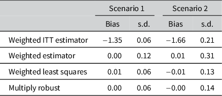We repeat each scenario for 1,000 total iterations. Table 1 displays the results for the four estimators when $N + n = 5,000$ , under two settings where $n/(n + N) \approx 0.71$ or $n/(n + N) \approx 0.23$ .

Table 1

The bias and standard deviations of the weighted estimator, WLS estimator, multiply robust estimator and the weighted ITT estimator

Table 1 Long description

We compare the bias/standard deviations of the weighted ITT estimator, weighted T-CACE estimator, weighted least squares T-CACE estimator, and a multiply robust estimator. The weighted ITT estimator is biased, while the other 3 are unbiased across the simulations. We see that WLS and multiply robust perform comparably and provide some efficiency improvements over just weighting.

Note: The results are based on 1,000 trials with a total sample size of $N + n = 5,000$ . Scenario 1 represents $n/(n + N) \approx 0.71$ , while scenario 2 corresponds to $n/(n + N) \approx 0.23$ .

6.2 Simulation results

Overall, we see that the mean errors of $\widehat {\tau }_{w}, \widehat {\tau }_{\text {wls}}$ and $\widehat {\tau }_{\text {mr}}$ are negligible, highlighting the consistency of the underlying estimators. The weighted ITT estimator that does not account for compliance is biased downward, suggesting that the causal effect is stronger among the compliers in the target population. Furthermore, the WLS and multiply robust estimators exhibit substantially smaller variances than the weighted estimator.

Finally, we evaluate the performance of the different estimators under more complex settings. Section F.2 of the Supplementary Material compares the performance of the principal stratification estimators defined in Theorem 2 of Clark et al. (Reference Clark, Rott, Hodges and Huling2024) with the WLS estimators. We find that in scenarios where principal ignorability is violated due to unmeasured confounders affecting both treatment received and outcome, the WLS estimator remains robust as the dimensionality of the unobserved variables increases, while the principal stratification estimator suffers from systematic bias. In Section F.3 of the Supplementary Material, we conduct extensive experiments under the setting of an observational study. We further evaluate the proposed sensitivity analysis framework in Section F.4 of the Supplementary Material.

7.1 Setting 1: Generalizing to participants who did not take the follow-up survey

We begin by generalizing the results to the set of participants who did not take the follow-up survey. While we have a measure of compliance for some of the individuals in the target group, we do not have access to their outcomes. For each voter, we have access to 33 total pre-treatment covariates that include demographic information, such as age, gender, past electoral participation as well as 25 survey items measuring immigrant-related opinions prior to treatment. We apply our weighted estimator and WLS estimator to generalize the CACE from the study sample to these participants.

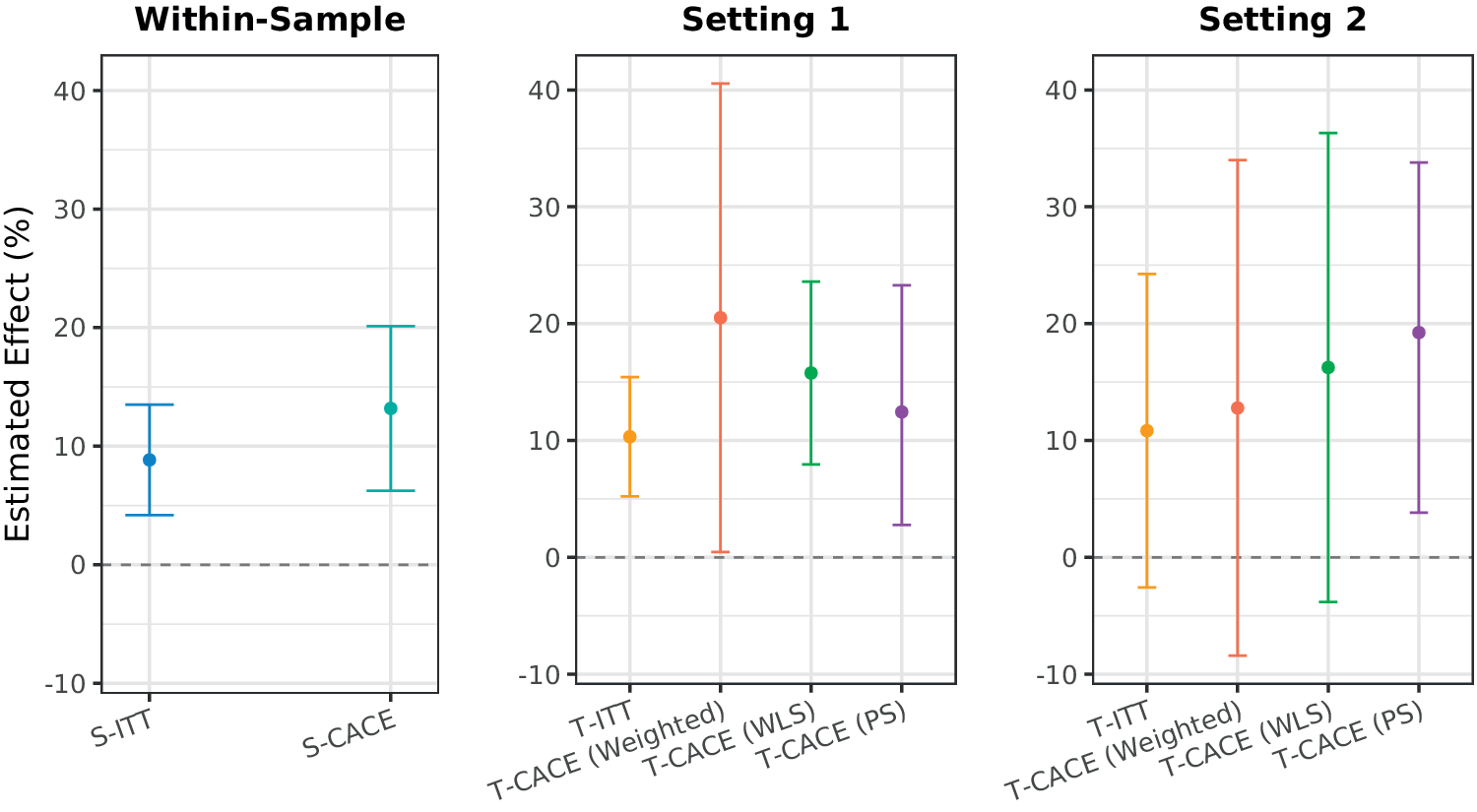
The estimated T-CACEs range from 12% to 20%. Notably, the results for the weighted and WLS T-CACE estimators are statistically significant at the 5% level. We also include the principal stratification estimator (weighted [PS]) introduced in Section F.2 of the Supplementary Material, which is based on the principal ignorability assumption. It provides a comparable estimate to our methods: $(12.4\%; [2.8, 23.3]).$ Taken together, these estimates provide robust evidence that deep canvassing positively influenced the target index, with some variation in magnitude across estimation methods. The generalized CACE in this context is larger than the generalized ITT $(10.3\%; [5.2, 15.4])$ and comparable to the within-sample CACE estimate $(13.2\%; [6.2,20.1]).$ This suggests that the estimated treatment effect on support for unauthorized immigrants from deep canvassing generalizes well to the population of individuals who failed to participate in the follow-up survey.

7.2 Setting 2: Generalizing to voters who did not participate in the experiment

We now consider the harder task of generalizing to the set of individuals who did not respond to the initial recruitment survey. This consists of 209,730 registered voters. Unlike the first setting, we are restricted to basic demographics, as the individuals who did not participate in the experiment failed to complete the baseline survey. As a result, we can only adjust for age, gender, location and past electoral participation history.

In contrast to the first setting, we find that, except for the PS estimator, T-CACE estimates are all statistically insignificant at the 5% level. We conclude that among the 209,730 voters who did not participate in the experiment, the impact of deep canvassing remains unclear at the 5% significance level. The larger intervals are likely due to the greater degree of imbalance between the study sample’s units and the target. This is in line with what we would expect intuitively, as there likely is a greater degree of distribution shift between individuals who did not participate at all in the experiment than those who initially participated, but failed to participate in the follow-up survey (i.e., Setting 1).

Figure 1 summarizes the results for these two settings, as well as the estimated within-sample effects, with numerical results in Table 7 in Section H.2 of the Supplementary Material. We provide an illustration of the sensitivity analysis in Section H.1 of the Supplementary Material.

Figure 1

Plot of various estimates and 95% confidence intervals for the deep canvassing application. The leftmost panel shows the within-sample effects. The middle panel displays results for participants who did not take the follow-up survey. The rightmost panel presents estimates for participants who did not participate in the experiment at all. We use the prefix “S-” to denote within-sample estimates and “T-” to denote the corresponding target quantities of interest.

Figure 1 Long description

The left-most panel shows the within-sample effects. The middle panel displays results for participants who did not take the follow-up survey. The right-most panel presents estimates for participants who did not participate in the experiment at all. Depending on the estimator used, the estimated T-CACE's vary in magnitude.