Implications
Most pig growth models are deterministic and predicted performance and derived nutritional recommendations do not account for variation of performance within a group. Adding stochasticity to these models requires not only knowledge of the variation in model parameters but also the covariance among parameters. This study focused on this covariance and the extent to which this information can be generalized across populations. The aim was to propose a generic covariance structure that will enable considering variation among individual pigs in growth modeling. Accounting for this variation is important to estimate the variation in nutritional requirements among pigs, and adopt feeding practices accordingly.
Introduction
Numerous studies have been performed to determine nutrient requirements in growing pigs. The concepts and knowledge developed over the years have been aggregated in mechanistic and dynamic nutritional growth models (e.g. Ferguson et al., Reference Ferguson, Gous and Emmans1994; van Milgen et al., Reference van Milgen, Valancogne, Dubois, Dourmad, Sève and Noblet2008). The characterization of the change in performance over time for the average pig is the first step required for the evaluation of nutrient requirements at the group level. Yet, applying feeding strategies based on the average pig to a group of pigs implies that requirement will be met for not more than 50% of the pigs in the group (Brossard et al., Reference Brossard, Dourmad, Rivest and van Milgen2009). Accounting for differences among pigs within a group is essential in precision farming, which can improve economic performance and reduce environmental impact (Pomar et al., Reference Pomar, Dubeau and van Milgen2009).
Deterministic growth models rely on the average response of the pigs. In contrast, stochastic models account for variability. They can provide more realistic responses, if the variability of the group can be described accurately. This variability is due to variation among individuals (related to genetic differences), or to variation of a given process over time for an individual (response to environmental or sanitary issues). The latter approach has been used by Strathe et al. (Reference Strathe, Sorensen and Danfaer2009) to build a model that includes daily variation in feed intake (DFI) and BW. However, calibration of such a model is complicated, and random processes make it difficult to obtain realistic ranges of parameters (Knap and Schrama, Reference Knap and Schrama1996). Variation among pigs can be modeled by using a deterministic growth model through performing repeated simulations based on different sets of parameters. These parameters can be generated by multivariate random processes using the means and covariance structure of parameters (Ripley, Reference Ripley1987). However, information on covariance structure of parameters is scarce and often incomplete (Knap, Reference Knap1995). Thus, the population response has been modeled with repeated simulations for individual animals using independently generated parameters by Ferguson et al. (Reference Ferguson, Gous and Emmans1997) and Pomar et al. (Reference Pomar, Kyriazakis, Emmans and Knap2003), or with a hypothetic pattern of correlation or covariance between parameters by Wellock et al. (Reference Wellock, Emmans and Kyriazakis2004b) and Morel et al. (Reference Morel, Wood and Sirisatien2008).
Including stochasticity in growth models increases the information requirement on variability and covariance of parameters. The first step to do this is to consider the phenotypic variability in healthy pigs reared in a controlled environment. The objective of this study is (1) to provide knowledge on the covariance structure of model parameters in different groups of pigs and (2) to identify the extent to which this information can be generalized across groups. This will help to include stochasticity in growth models by providing a generic covariance structure to be used to generate populations with realistic variation and relations between individual parameters.
Material and methods
Experimental design and measurements
Experimental data on the change in DFI and BW were obtained for gilts and barrows for which performance was recorded between ∼30 and 110 kg. The data originated from 10 batches of 144 pigs each that were raised at the experimental facilities of IFIP (Romillé, France) between May 2007 and September 2011. Within each batch, 36 barrows and 36 gilts were obtained from Large White × Landrace (LW × LD) sows inseminated with semen from crossbred Large White × Pietrain (LW × PP) sires. The other 36 barrows and 36 gilts within a batch were obtained from one of eight other lines of sires used in this study: Pietrain (PP, batches A and B), Pietrain × Duroc (PP × Du, batch C), Duroc (Du, batches D and E), four commercial synthetic lines (SL1 to SL4, batches F, G, H and I), or Large White dam line (LW, batch J). The experiment started after a 1-week adaptation period to the housing conditions, that is, 1 week after pigs were transferred from post-weaning unit to fattening unit. Pigs left the facilities at ∼110 kg BW to be slaughtered. The study was conducted in accordance with the French legislation on animal experimentation and ethics. The certificate of Authorization to Experiment on Living Animals no. 35-07 was delivered by the French Ministry of Agriculture to N. Quiniou to conduct experiments at the IFIP facilities in Romillé (France).
Housing and feeding conditions
For each batch, two similar experimental rooms of six pens each were used. The pens were equipped with concrete slatted floor and housed six gilts and six barrows from the same crossbreed each. Pigs were allotted to the pens at 60 days of age based on dam, sire and BW. The objective was to study penmates that originated from not more than three different litters within a pen and to avoid pigs weighing <18 kg to make sure they could use the feeding stations. Then, heaviest pigs were also excluded from the candidates. When the pigs weighed < 27 kg on average, they stayed for 1 additional week in the post-weaning unit. Pigs from six batches were transferred at 61 days of age in the fattening unit, whereas pigs from the other four batches stayed 7 additional days in the post-weaning rooms. On average, the experiment started at 70 days of age. Each room housed three pens of (LW × LD) × (LW × PP) progeny and three pens of the alternative crossbreed. Pigs had ad libitum access to feed and water through the experiment. The dietary net energy (NE) content was fixed to 9.7 MJ/kg, whereas the standardized ileal digestible lysine contents were 0.90 and 0.80 g/MJ NE in diets provided before or after 70 kg BW, respectively. Diets were formulated to meet or exceed French nutritional recommendations (IFIP, 2000). Ambient temperature was regulated similarly for both rooms; during the first 14 days, it decreased from 25°C to 22°C, and was kept constant at 22°C thereafter.
Feed intake and growth
Animals were weighed at 60 days of age and at the beginning of the control period (i.e. after the adaptation period of 1 week), every 3 weeks until 100 kg BW and every 2 weeks thereafter. The DFI was measured individually through an automatic feed dispenser (Acema 64, Acemo, Pontivy, France), as described by Labroue et al. (Reference Labroue, Guéblez, Sellier and Meunier-Salaün1994). Two potential problems can occur with electronic feeders: feed disappearance and identification of pigs (Casey et al., Reference Casey, Stern and Dekkers2005). Each week, total feed disappearance from the dispenser was measured manually and compared with the sum of individual DFI records. When the difference was >4%, the recorded DFI during this 7-day period was corrected accordingly. When feed intake was not attributed and a posteriori identification was possible (e.g. because of a pig having lost its ear tag), DFI was attributed to the identified pig. Otherwise, the unattributed DFI was attributed equally among the penmates. The total number of individual DFI measurements (or pig-days) corresponded to 131 655 records. Among these pig-days, 4% were manually attributed to individual pigs and 17% were attributed equally to all penmates. Identification errors explained the majority of this attribution (17% of the records), which is consistent with values of Casey et al. (Reference Casey, Stern and Dekkers2005; 4% to 19% across three successive experiments). For each pig, the average DFI (ADFI) was calculated as the sum of individual DFI during the whole experiment divided by the duration of the experiment. The feed conversion ratio (FCR) was calculated individually as the ratio between total feed intake and BW gain.
Within each batch, pigs were slaughtered in one, two or three groups (i.e. all at the same day, or 7 or 14 days apart). The expected BW on the slaughter day was estimated from the average daily gain (ADG) measured over the previous 2-week period. Pigs were slaughtered when they weighed at least 103 kg the day before slaughter. These animals were fasted from 0800 h, weighed at 1400 h and slaughtered at 0800 h the next day. At slaughter, the depths of backfat (F34) and Longissimus dorsi muscle (M34) were measured between the third and fourth last ribs with an invasive probe (Capteur Gras Maigre, Sydel, Lorient, France). The lean content (%) of the carcass was calculated from F34 and M34 (mm), using the equation commonly used in French slaughter plants: 62.19 – 0.729 × F34 + 0.144 × M34 (Daumas et al., Reference Daumas, Causeur and Predin2010).
Performance and carcass data were submitted to a multifactorial ANOVA with sex (two levels), batch (10 levels), crossbreed within batch (nine levels) and interactions as main effects (proc MIXED; SAS, 2000). The pig was considered as the experimental unit and the pen within a batch as a random effect. Carcass traits were analyzed using BW at slaughter as a covariate.
Model parameters describing feed intake and growth
A Broyden–Fletcher–Goldfarb–Shanno optimization method was used to fit simultaneously the DFI and BW equations to data using the InraPorc (2006) model. Feed intake was modeled as a gamma function of BW:
 $${\rm{DFI}}\,{\rm{(MJ}}\,{\rm{NE/day)}} = {{a}}\times {{(b}}\times {\rm {BW}}\times {{{{e}}}^{ - {\rm{b}}\times {\rm{BW}}}} + {\rm{1)}}\times {{c}}\times {\rm{B}}{{{\rm{W}}}^{{\rm{0}}{\rm{.60}}}} $$
where ‘a’ (dimensionless) and ‘b’ (per kg) are parameters and ‘c’ is a constant (0.75 MJ NE/kg BW0.60 per day). With this function, feed intake is described as multiples of the NE intake above maintenance, so that the pig eats for maintenance when it reaches maturity. The expected DFI at 50 (DFI50) and 100 kg (DFI100) were used to replace parameters ‘a’ and ‘b’. The growth curve was parameterized using three parameters: BW at 70 days of age (BW70, kg), mean protein deposition rate between 70 days of age and 110 kg BW (PDm, g/day), and the shape parameter of the Gompertz function (BGompertz, per day) describing the precocity of protein deposition (PD). These three parameters determine the Gompertz function used to model PD (see van Milgen et al. (Reference van Milgen, Valancogne, Dubois, Dourmad, Sève and Noblet2008) for detailed equations and for the relation between BW and PD). When control started after 70 days of age, BW70 and PDm were obtained by extrapolating data between the age at control start and 70 days. The set of five parameters describing the feed intake and growth curves of an individual pig is referred to hereafter as the profile. The duration of the experiment from 70 days of age to 110 kg BW (duration) was also calculated, even though it is not required to characterize the pig (i.e. it is a function of the other model parameters).
Forty-eight pigs died or were removed from the pens before slaughter because of sanitary issues. Animals recorded with sanitary issues during the data collection (n = 19) were also excluded because they may not have been capable to express their growth phenotypic potential. For some other pigs (n = 85), it was not possible to estimate model parameters because of calibration failure or unrealistic values for the estimated parameters (e.g. negative values of BGompertz or values of PDm >270 g/day). The threshold value for PDm corresponded to the highest maximum PD obtained in five genotypes by Knap (Reference Knap2000) that corresponds also to an outlier in PDm distribution in our study. In addition, individual cumulative feed intake and curves were graphically examined after calibration. Indeed, only the feed intake and growth potential were supposed to determine actual performance. When a discontinuous pattern of one of these curves was observed, reflecting a stagnation or loss of BW between two measurements or a period of several days of decreased feed intake, the concerned animals were excluded from the analysis even if calibration succeeded and realistic values were obtained. In total, calibration failures, unrealistic values, or discontinuous patterns of growth or intake concerned 152 profiles, which corresponded to 11% of all pigs studied. After successful estimation of model parameters, a total of 1288 profiles were retained.
Average parameters and their covariance
Parameter values of individual profiles were submitted to an ANOVA (proc MIXED; SAS, 2000), to evaluate the effect of sex, batch, crossbreed and their interactions; the pig was considered as the experimental unit and the pen within a batch as a random effect. Correlation and covariance relationship between parameters were described with a dual multiple factorial analysis (DMFA; Lê et al., Reference Lê, Husson and Pagès2007). This method is based on the same principles as the principal component analysis, and deals with the structure of data segregated in several populations. The DMFA allows for identification of the constant relations across populations by scaling values per population. This eliminates the bias introduced by differences in parameter mean and variance across populations. The DMFA reduces the possible bias introduced by the over-representation of LW × PP progenies in the data set. The individual profile parameters are projected on planes composed of two principal components. The correlation between two parameters is described through the angle between their respective projections. The ADG, ADFI, FCR, backfat thickness and lean content were also projected to illustrate the relation between the structure of parameters and the observed performance. It allowed for the calculation of the constant correlations between profile parameters and performance traits across populations.
Comparison of covariance matrices
On the basis of the characteristics of the data set, subpopulations were defined according to batch, sex, crossbreed and their combinations, and covariance matrices were computed for each subpopulation. The CPC program (Phillips and Arnold, Reference Phillips and Arnold1999) for common principal components analysis was used to compare covariance matrices of subpopulations on the basis of proximity of the covariance pattern from one matrix to another according to the Flury hierarchy (Reference Flury1988). This multidimensional approach allows defining different levels of proximity among matrices, which is more accurate compared with the usual segregation that considers only equality v. difference. Two covariance matrices can be described as unrelated, or they can present a common first principal component, two first principal components, etc. They can also present the same principal components while being equal or proportional. The covariance matrices for the studied subpopulations were compared depending on the grouping criteria used: batch, sex, crossbreed and their combinations. Two subpopulations can be considered as similar, if they share all their principal components (Boente et al., Reference Boente, Rodriguez and Sued2010).
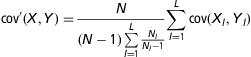
It is possible that the analysis described above will indicate that all subpopulations of pigs are different. This would imply that information about the variation would have to be obtained for each population of pigs. Although this would be most appropriate from a statistical point of view, it would be very difficult to implement. We therefore also evaluated a generic covariance matrix that would be most appropriate (or least inappropriate), if the results of our experiment indicated that each population had its own variance structure. Two generic matrices were calculated to elaborate a single matrix that would represent the entire data set. The first generic matrix, or raw matrix, was computed from the 1288 individual profiles without any reference to the population definition. The second matrix was calculated as a sum of the 40 covariance matrices, each obtained from the specific subpopulation defined by the combination of batch (10 levels), sex (two levels) and crossbreed within a batch (two levels within each batch; i.e. a matrix by sex and by crossbreed within each batch), corrected by a scale value (equation 1). This scale value depended on the total number of pigs and on the number of pigs in each subpopulation. The aim was to give the same importance to each subpopulation, regardless of its size. It was supposed to be scaled by group, and not to show the differences in correlation levels among groups. This matrix was considered as a mean matrix that would be in a central position among the matrices from all subpopulations.
The following equation calculates the generic term of mean covariance matrix (cov′) from values of the generic terms of specific group (l) covariance matrix (cov). N is the total number of individuals (1288) and Nl the number of individuals in the specific group l (40 groups):
 $${\rm{cov}}'\left( {X,Y} \right) = \frac{N}{{\left( {N - 1} \right)\mathop{\sum}\limits_{l = 1}^L {\frac{{{{N}_l}}}{{{{N}_l} -1}}} }}\mathop{\sum}\limits_{l = 1}^L {{\rm cov}\left( {{{X}_l},{{Y}_l}} \right)} $$
The raw and the mean matrices were each compared with the 40 subpopulation matrices, using the χ 2 distance from the equality v. unrelated test of the CPC program. This χ 2 distance was used to measure the accuracy of the tested matrix as an estimator of the observed covariance through the mean χ 2 distance calculated from the 40 χ 2 distances computed between the tested matrix and each of the 40 covariance matrices.
Results
Feed intake and growth
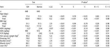
Pigs from the different batches were moved to the fattening rooms at 61 or 68 days of age, and the experiment began at 68 or 75 days. The batch significantly affected all traits (Table 1). Therefore, it was not possible to compare all crossbreeds together, but this effect was tested within the batch. With this experimental design, the crossbreed had effect on age at the beginning of the experiment (P < 0.01), final BW (P < 0.01), hot carcass weight (P < 0.01), muscle depth (P < 0.01) and carcass leanness (P = 0.01; data not shown). The effect of crossbreed was non-significant (P ⩾ 0.10) or showed a tendency (P < 0.10) for other traits.
Average performance and carcass characteristics by sex of crossbred pigs obtained from nine different sire lines and controlled in 10 different batches during the grower–finisher phase (n = 1288)Footnote 1

B = batch; S = sex; C = crossbreed within batch; ADFI = average daily feed intake; ADG = average daily gain; FCR = feed conversion ratio.
1 ANOVA with B, S, C and the interactions B × S, S × C as main effects, and pen within batch as random effect (proc MIXED, SAS). Two crossbreeds were compared within each batch, and batch effect was significant for all traits, so that the crossbreed effect was tested within batch. As the differences between sexes differed among crossbreeds, only the sex average is indicated.
2 Available for 646 gilts and 639 barrows.
Barrows were on average 0.4 kg heavier than gilts at the beginning of the experiment (Table 1). Barrows had also greater ADG (972 v. 904 g/day for gilts; P < 0.01) and ADFI (2.54 v. 2.24 kg/day; P < 0.01). This resulted in a greater FCR (2.62 v. 2.52; P < 0.01) and fatter carcasses (58.6% v. 61.1% lean; P = 0.01) for barrows than for gilts. These differences between sexes changed from a batch to another or from a crossbreed to another, resulting in a significant interaction of sex with crossbreed and batch.
Average value of parameters that describe the animal profiles
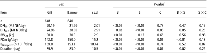
The parameter estimates describing individual pigs differed significantly among the subpopulations, according to batch, sex and crossbreed (Table 2). The average BW70 per subpopulation ranged between 27.1 and 34.0 kg, and was affected by batch (P < 0.01). A batch effect was also observed for BGompertz (P < 0.01, with values ranging between 0.0129 and 0.0256/day), for PDm (P < 0.01, with values ranging between 130 and 166 g/day), for DFI50 (P < 0.01, with values ranging between 18.6 and 24.0 MJ NE/day) and for DFI100 (P = 0.02, with values ranging between 23.7 and 31.2 MJ NE/day).
Estimates of model parametersFootnote 1 describing the change in feed intake and BW in crossbred pigs obtained from nine different sire lines and controlled in 10 different batches during the grower–finisher phase (n = 1288)Footnote 2
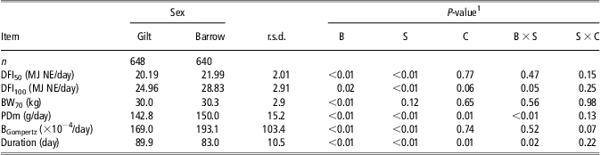
B = batch; S = sex; C = crossbreed within batch; DFI = daily feed intake; NE = net energy.
DFI50 and DFI100: feed intake at 50 or 100 kg BW; duration: duration of experiment from 70 days of age to 110 kg BW. BW70: BW at 70 days; PDm: mean protein deposition rate between 70 days of age and 110 kg BW; BGompertz: precocity of protein deposition curve.
1 DFI was modeled by a gamma function of BW (see details in text) using the parameters DFI50 and DFI100. The growth curve was parameterized using three parameters: BW70, PDm and the shape parameter of the Gompertz function describing the precocity of protein deposition curve (BGompertz). These three parameters determine the Gompertz function used to model protein deposition using the InraPorc model (van Milgen et al., Reference van Milgen, Valancogne, Dubois, Dourmad, Sève and Noblet2008).
2 ANOVA with B, S, C and the interactions B × S, S × C as main effects, and pen within batch as random effect (proc MIXED, SAS). Two crossbreeds were compared within each batch, and batch effect was significant for all traits, so that the crossbreed effect was tested within batch. As the differences between sexes differed among crossbreeds, only the sex average is indicated.
No effect of crossbreed was observed for the model parameters (P > 0.06) except for PDm (P = 0.01). Greater DFI50 and DFI100 were observed for barrows than for gilts (22.0 v. 20.2 MJ NE/day, and 28.8 v. 25.0 MJ NE/day, respectively; P < 0.01). A similar BW70 was obtained for barrows and gilts. In contrast, duration was shorter for barrows than for gilts (83.0 v. 89.9 days, P < 0.01) in relation to a greater PDm (150 v. 143 g/day, P < 0.01). The precocity parameter BGompertz was significantly greater for barrows than for gilts (0.0193 v. 0.0169/day, respectively; P < 0.01). Differences in PDm and DFI100 between sexes depended on the batch (interaction, P < 0.01 and P = 0.05, respectively).
Comparison of covariance matrices
When the covariance matrices were computed according to batch, crossbreed or their combinations, all subpopulations were identified as being unrelated by the CPC program (P < 0.01). The covariance matrices computed according to sex shared the principal components, but the different combinations of batch, sex and crossbreed to compute covariance matrices produced only unrelated matrices. However, some exceptions were obtained for specific comparisons. For instance, a similar covariance matrix was obtained for barrows and gilts in Batch A. The covariance matrices of two of the three synthetic lines also shared all principal components. The LW × PP and the PP progenies had the two first principal components in common. On the basis of these results, it was concluded that each subpopulation, defined by batch, sex and crossbreed was specific in terms of covariance structure.
The observed covariance structure
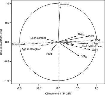
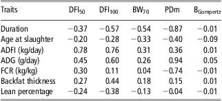
The relations among parameters were examined through within subpopulation correlations, as the subpopulations differed in terms of covariance. The results of the DMFA analysis (used to evaluate the part of correlation among parameters that would be common for the 40 populations) are represented in Figure 1 and correlations between parameters and performance traits are given in Table 3. Owing to the number of observations, all correlation coefficients differed from zero according to a Pearson correlation test (P < 0.01). More than 50% of inertia (i.e. of the common variability) was projected, and thus summarized on the first plane obtained with the DMFA analysis (Figure 1). Moreover, most of the parameters were well projected on the first plane indicating that their variability was summarized well on this plane. These elements indicated a strong correlation structure among parameters with the DMFA analysis. The DFI50 and DFI100 were both positively correlated to ADFI (r = 0.78 and 0.76, respectively), but DFI50 was more closely correlated with FCR than DFI100 (r = 0.30 and 0.11, respectively). In contrast, DFI50 was less correlated with ADG than with DFI100 (r = 0.45 and 0.60, respectively). The same result was obtained for the correlation with duration (r = −0.37 and −0.57, respectively), backfat thickness (r = 0.27 and 0.44, respectively) and lean percentage (r = −0.24 and −0.38, respectively). Duration and PDm were negatively and strongly correlated (r = −0.87). The PDm was moderately correlated to DFI100 (r = 0.40), whereas the correlations with DFI50 (r = 0.20) and BW70 (r = 0.24) were lower. In contrast, the correlation with ADG was greater (r = 0.94). The BGompertz was not related to the other parameters, as its projection on the first plane was weak, it was the only parameter well projected on the second component and its correlation with other parameters was low (maximum r = 0.06).
Correlations between parameters used to model feed intake and BW of crossbred pigs obtained from nine different sire lines and controlled in 10 different batches during the grower–finisher phase (n = 1288). Plot from dual multiple factor analysis1; solid arrows represent the average projection of the model parameters1 (DFI50 and DFI100: daily feed intake at 50 or 100 kg BW; BW70: BW at 70 days; PDm: mean protein deposition rate between 70 days of age and 110 kg BW; BGompertz: precocity of protein deposition curve); dotted arrows represent performance traits (ADFI: average daily feed intake; ADG: average daily gain; FCR: feed conversion ratio).1 Plot of the projection of parameters on the first plane obtained by dual multiple factor analysis. This plane summarized more than 50% of inertia, that is, of the common part of variation among the 40 groups of pigs determined by the combination of sex, batch, and crossbreed.2 DFI was modeled by a gamma function of BW (see details in text) using the parameters DFI50 and DFI100. The growth curve was parameterized using three parameters: BW70, PDm, and the shape parameter of the Gompertz function describing the precocity of protein deposition (BGompertz). These three parameters determine the Gompertz function used to model protein deposition using the InraPorc model (see van Milgen et al., Reference van Milgen, Valancogne, Dubois, Dourmad, Sève and Noblet2008).

Correlations between model parameters describing the change in feed intake and BWFootnote 1 and observed performance traits of crossbred pigs obtained from nine different sire lines and controlled in 10 different batches during grower–finisher phase (n = 1288) Footnote 2
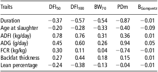
DFI = daily feed intake; ADFI = average daily feed intake; ADG = average daily gain; FCR = feed conversion ratio.
DFI50 and DFI100: feed intake at 50 or 100 kg BW (MJ NE/day); BW70: BW at 70 days (kg); PDm: mean protein deposition rate between 70 days of age and 110 kg BW (g/day); BGompertz: precocity of protein deposition curve (per day).
1 Daily feed intake was modeled by a gamma function of BW (see details in text) using the parameters DFI50 and DFI100. The growth curve was parameterized using three parameters: BW70, PDm and the shape parameter of the Gompertz function describing the precocity of protein deposition curve (BGompertz). These three parameters determine the Gompertz function used to model protein deposition using the InraPorc model (see van Milgen et al., Reference van Milgen, Valancogne, Dubois, Dourmad, Sève and Noblet2008).
2 Correlations were obtained through a dual multiple factor analysis, from groups defined by the combination of batch, sex and crossbreed.
The correlations between parameters were variable from a subpopulation to another. The correlation between DFI100 and PDm was similar for the subpopulations (0.29 ⩽ r ⩽ 0.63, 50% CI) This was also the case for the correlations between DFI50 and PDm (0.12 ⩽ r ⩽ 0.51), DFI100 and BGompertz (−0.68 ⩽ r ⩽ −0.29), and DFI50 and DFI100 (−0.14 ⩽ r ⩽ −0.26) or BGompertz (−0.74 ⩽ r ⩽−0.29). In contrast, the correlation between DFI50 and BW70 was variable for the different subpopulations (−0.36 ⩽ r ⩽ 0.25), as were correlations between BGompertz and PDm (−0.14 ⩽ r ⩽ 0.43), and between BW70 and BGompertz (−0.49 ⩽ r ⩽ 0.05), or PDm (0.03 ⩽ r ⩽ 0.53), or DFI100 (−0.16 ⩽ r ⩽ 0.34).
Comparison of generic covariance matrices
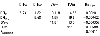
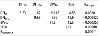
The χ 2 distance between the 40 matrices of the subpopulations and the generic matrices was smaller for the median covariance matrix than for the raw covariance matrix (mean χ 2 distance between subpopulations matrices and generic matrix of 55 for the median covariance matrix v. 59 for the raw covariance matrix, P < 0.01). It corresponded to a reduced deviation from the observed covariance matrices obtained from the 40 subpopulations. Simultaneously, the prediction was more accurate for 72% of subpopulations matrices with the median covariance matrix. The median covariance matrix is presented in Table 4. Values of obtained variance corresponded to coefficient of variation (CV) of 5% for DFI50, 6% for BW70 and DFI100, 11% for PDm and 58% for BGompertz.
The median covariance matrix among parametersFootnote 1 used to describe the change in feed intake and BW of crossbred pigs obtained from nine different sire lines and controlled in 10 different batches during the grower–finisher phase (n = 1288)
DFI = daily feed intake.
The covariance matrix contains variances (on the diagonal) and covariances (upper part). Matrix is obtained as a sum of covariance matrices from 40 populations separated by sex, batch and crossbreed, and scaled by a parameter depending on the number of populations.
DFI50 and DFI100: feed intake at 50 or 100 kg BW; BW70: BW at 70 days of age; PDm: mean protein deposition rate between 70 days of age and 110 kg BW; BGompertz: precocity of protein deposition curve.
1 DFI was modeled by a gamma function of BW (see details in text) using the parameters DFI50 and DFI100. The growth curve was parameterized using three parameters: BW70, PDm and the shape parameter of the Gompertz function describing the precocity of protein deposition (BGompertz). These three parameters determine the Gompertz function used to model protein deposition using the InraPorc model (see van Milgen et al., Reference van Milgen, Valancogne, Dubois, Dourmad, Sève and Noblet2008).
Discussion
Although the data were obtained from a single experimental farm, a wide range in performance data was obtained for pigs of different crossbreeds and sexes. Most model parameters were affected by batch, especially the characteristics of pigs at the beginning of the fattening period. Differences in BW70 resulted from differences in ADG during the preceding physiological stages. A significantly lower BW70 was observed for batches of pigs that were born, suckled or weaned in summer or early fall. During the lactation period, the growth rate of piglets depends on the milk production of sows, which is influenced mainly by ambient temperature (Black et al., Reference Black, Mullan, Lorschy and Giles1993). Ambient temperature was controlled in the experimental fattening rooms, but not in the lactation and post-weaning units, leading to possible differences in performance during this period. No significant differences in model parameters for growth were found among the crossbreeds. Similar results have been reported by Ferguson and Kyriazis (Reference Ferguson and Kyriazis2003) and Green et al. (Reference Green, Brotherstone, Schofield and Whittemore2003), who also compared different crossbreeds obtained from LW, LD or LW × LD sows. These authors suggested that the limited number of observations per subpopulation can result in a high variability of the parameters. Despite a greater number of pigs for each crossbreed in the present study, this was not sufficient to demonstrate differences among crossbreeds. The experimental design used in this study may also explain this result. Crossbreeds were all compared with a common control combination based on LW × PP sires.
The DFI50 and DFI100 of different types of pigs have been described by van Milgen and Noblet (Reference van Milgen and Noblet1999) using an asymptotic equation. Converting their data on a NE basis, the DFI50 ranged, respectively, from 16.6 to 18.6 MJ NE/day for PP boars and boars from a synthetic line, which was similar to the SL1 sire used in the present experiment. The differences were even greater for DFI100, as corresponding values were 21.6 and 26.3 MJ NE/day. In the present study, the differences in DFI50 and DFI100 between crossbreeds obtained from PP or SL1 sires were, respectively, 0.23 and 1.27 MJ NE/day in gilts, and 0.52 and 0.57 MJ NE/kg in barrows. These small differences in parameters describing the DFI curve are consistent with the absence of differences in ADFI. The differences between our results and those of van Milgen and Noblet (Reference van Milgen and Noblet1999) may be because of the choice of the equation used to describe DFI. Moreover, in the present study, the design of crossbreed including 50% of LW × LD type can attenuate the differences between crossbreeds in the DFI pattern.
Accurate characterization of animals
The gamma function was used to describe DFI, which was shown to fit DFI better than other feed intake equations such as linear, power or exponential functions (Vautier et al., Reference Vautier, Quiniou, van Milgen and Brossard2011). It was preferred because it allows for a decline in feed intake with increasing BW. This is consistent with the concept that a mature, non-producing animal should eat for maintenance. The interest of the Gompertz function to model PD has been discussed by van Milgen et al. (Reference van Milgen, Valancogne, Dubois, Dourmad, Sève and Noblet2008). The Gompertz function requires only three parameters, which is interesting with respect of the principle of parsimony (Wellock et al., Reference Wellock, Emmans and Kyriazakis2004a).
The advantage of using a mechanistic modeling is that the resulting parameters can be interpreted from a biological perspective. The DFI50 and DFI100 are partial indicators of the ADFI. The BW70 is used as an initial condition for simulation and is reliable to performance in preceding stages. The BGompertz describes the sigmoid evolution of PD rate when BW increases. The PDm is an indicator of the average growth potential during the period of calibration, instead of the protein mass at maturity used in the Gompertz function (Emmans and Fisher, Reference Emmans and Fisher1986). It is closely linked to ADG in the present study (r = 0.94) because of model assumptions, illustrating the role of PD as a driving force of BW growth (Whittemore et al., Reference Whittemore, Kerr and Cameron1995; van Milgen et al., Reference van Milgen, Valancogne, Dubois, Dourmad, Sève and Noblet2008).
Definition and description of a population
To generate a virtual population of pigs where each pig has its proper characteristics, the mean values of model parameters must be known, in addition to the covariance structure of model parameters. With regard to the significant influence of the batch and sex, mean parameters should be estimated for each group. However, an a priori knowledge of performance is not possible for a given batch on commercial farm. On-farm estimation of model parameters by sex on the basis of feeding strategy (ad libitum preferentially), ADG and slaughter data would be useful to obtain a minimum of information. However, as shown in this study, the important batch effect may limit the use of historical data for prediction purposes.
Including stochasticity in growth models can be performed by repeating simulations with a deterministic growth model. Each simulation is then based on a different set of parameters characterizing different animals in population. These parameters can be generated by multivariate random processes using the means and covariance structure of parameters (Ripley, Reference Ripley1987). As information on variation and covariance of parameters are scarce, pig populations have been generated by considering parameters as independent (Ferguson et al., Reference Ferguson, Gous and Emmans1997; Pomar et al., Reference Pomar, Kyriazakis, Emmans and Knap2003) or with a hypothetic pattern of correlation or covariance between parameters (Wellock et al., Reference Wellock, Emmans and Kyriazakis2004b; Morel et al., Reference Morel, Wood and Sirisatien2008). However, the simulated variation is typically overestimated when covariance among parameters is not taken into account. Traits such as ADG and DFI, and thus parameters used to describe them in models, are correlated and some of the variation in these traits is shared (Pomar et al., Reference Pomar, Kyriazakis, Emmans and Knap2003). To account for variability in performance by modeling, the covariance matrix of model parameters has to be known (Pomar et al., Reference Pomar, Kyriazakis, Emmans and Knap2003). In the current study, the CPC tests indicated differences in covariance structure among the 40 subpopulations, defined by the combination of batch, sex and crossbreed. From a statistical point of view, one should then evaluate a specific covariance matrix for each group of pigs. Real-time, on-farm estimation of the covariance matrix structure is not realistic and using the median covariance matrix is proposed as an alternative. Simple specific correlations have been described by Ferguson et al. (Reference Ferguson, Gous and Emmans1997) such as the correlation between BGompertz and protein mass at maturity. Morel et al. (Reference Morel, Wood and Sirisatien2008) have also proposed a covariance matrix with three parameters: potential for maximum PD, daily energy intake and the minimum ratio between lipid deposition and PD. However, these correlations were specific to their study. In the present study, the median covariance matrix was designed as a generic matrix to represent variation in a group of pigs between feed intake and growth parameters, as it integrated the differences in covariance matrices among different subpopulations. The covariance between parameters was consistent with the common pattern of correlations observed among groups, with a positive covariance between PDm and feed intake parameters and between PDm and BW70, and a negative covariance between BW70 and DFI50 and between BGompertz and DFI50 and DFI100. The CV for PDm (11%) was consistent with CV values ranging between 4% and 33% for maximum PD rate as collected by Knap (Reference Knap2000) from literature; but the high CV for BGompertz in this study exceeded the maximum of 41% reported by this author. The variation in DFI50 and DFI100 in the present study (CV of 5% to 6%) was similar to values reported by van Milgen and Noblet (Reference van Milgen and Noblet1999).
The proposed median covariance matrix showed a better ability than the raw covariance matrix to represent the covariance in different subpopulations. In the end, the median matrix presented should be preferred for the multivariate random generation of individuals for simulation, even if it may not be completely accurate. Considering a realistic covariance among model parameters will allow generating virtual populations of pigs having a realistic variation. Simulating performance of such populations will help to consider more precisely the effect of different nutritional strategies on mean performance but also on their variation. However, obtaining this information is currently not possible and the median covariance is the most suitable alternative.
Conclusion
This study illustrates the difficulty to account for variation in pig populations, because this variation not only exists within a population, but also among populations. In order to overcome this difficulty, we identified a common covariance pattern of growth model parameters through different groups. This approach is to be preferred over one where model parameters are assumed to be independent. Each population can then be represented by a vector of the mean values of parameters, which needs to be obtained for each production setting, and the generic covariance matrix proposed in this study. Although the approach developed here was used for a specific growth model, it can be applied to other mechanistic growth models.
Acknowledgments
This study was performed on behalf of the mixed technological unit (UMT) “Engineering for pig production systems” and was funded by the French Ministry of Agriculture, Food, Fisheries, Rural Affairs and Spatial Planning. B. Vautier gratefully acknowledges the ANRT, on behalf of the French Ministry of Higher Education and Research for partly supporting his PhD work.