

1. Introduction
Johannes Kepler (1571–1630) is well known for his work on celestial mechanics and stereometry. His achievements in astronomical research reached beyond the three laws on which his fame mainly rests today. It should be remembered that Kepler was active before calculus was invented by Newton and Leibniz, but even without the aid of a formal calculus, he was able to arrive at many important results for natural philosophy. He was the first natural philosopher whose analysis reached laws of nature in the modern meaning of the word: they were empirical, physical, and stated in mathematical terms, rather than primarily philosophical or pure mathematical ideas. His resulting work is considered to be an important contribution in the development of pre-calculus. Further, he posed many interesting problems that posed challenges in the years to come, and defining a problem is often as important as eventually solving the problem.
Like many of the leading natural philosophers before him, Kepler had a profound feeling for the harmony of the universe, and he saw his work as a God-given mission to understand the divine work and structure of creation.Footnote 1 His basic contributions to astronomy and astrophysics have been well studied (Beer and Beer Reference Beer and Beer1975; Stephenson Reference Stephenson1987; Davis Reference Davis1992). The tradition in which Kepler was trained made it natural for him to operate according to the principles of Aristotelian physics. But contrary to Aristotle, he also applied the principle of grounding astronomy in physics, and by doing this, he increased the use of physical methods. This involved the merging of two traditionally distinct disciplines, and instead of the usual approach of fixing the mean position of the sun, he fixed the actual position of the sun. In his pre-Newtonian physics, force was proportional to velocity, and Kepler treated a planet's orbit as the result of two forces: one rotating circumsolar like a “windmill,” and the other librational because it regulated the distance from the sun to the planet on the basis of a kind of planetary magnetism. These forces were strictly independent and mutually perpendicular, and Kepler was able to quantify them separately. In this way Kepler created a two-cause theoretical description of planetary motion in the solar system, and hence Copernican principles were for the first time implemented in firm astronomical practice.
Kepler was also a very able mathematician, and made important contributions to many different fields in mathematics (Belyi Reference Belyi1975; Costabel Reference Costabel1975). The summations that he carried out to determine the maximum capacity of wine barrels, and the volumes of other bodies, are widely known (Stereometria 1615). His efforts in this field were an extension of the work of Archimedes. Moritz Cantor called it – perhaps with some exaggeration – “the source and the inspiration for all later cubatures” (Cantor Reference Cantor1894, Vol. II, 823). In contrast to the Greek tradition, Kepler and other mathematicians of the 1600s started to dissect a given area or volume into an apparently infinite number of infinitesimal pieces, of a size and shape convenient to the solution of the problem. As a new tool in geometry, the concept of infinitesimals played an important role.
In many arithmetic books from the 1500s, one also finds the classical numeric method called regula falsi (rule of false position) to solve linear equations by a trial-and-error procedure. Any remark of the restriction to the linear case is often lacking, although some authors were clearly aware of this limitation (Smeur Reference Smeur1978).
Logarithms, which were discovered by John Napier (1550–1617), spread rapidly within mathematics during the years 1614–1630. Logarithms were exploited by natural philosophers like Kepler to speed up calculations. Kepler was deeply impressed by the discovery when he got a copy of Napier's book in 1619. Lacking any description of their construction, he recreated his own tables by a new procedure. Kepler's logarithms were different from Napier's work, which had started from visible geometric notions. Contrary to this, and to his normal preference for geometry, Kepler derived his numbers purely arithmetically by starting from the theory of proportions. Some years afterward he published his own theory and tables Chilias logarithmorum, composed in 1621–1622 and printed in 1624. Napier also invented mechanical devices to be used in his calculations, the so-called “Napier's bones” (Williams Reference Williams1983, 280–283). The name “bone” is related to the fact that the best material to be used for these mechanical devices was bone-like, such as ivory. They were used to do multiplication and extract square and cube roots.
Kepler was operating for the most part in a long-standing tradition of numerical calculation in astronomy, where astronomy was considered a branch of mathematics or geometry, with limited relationship to physics. The standard activity of the mathematical astronomers were abstract mathematics combined with the discipline of calculating the positions of the planets, and in this respect Kepler's work was as much about a new astronomical methodology as a new planetary theory. In his work, Kepler transcended the use of only geometrical tools as suitable in astronomy. From Tycho Brahe (1546–1601) he obtained a vast store of data, extending over more than 30 years of accurate naked-eye observations. As a natural philosopher Kepler was a committed problem solver. The new astronomy raised several problems that had to be worked out, and the main aim of the present paper is to show that Kepler's own justification of his astronomy was based on methods from numerical analysis. By these the non-circular geometry was made operational and computable several decades before the invention of the mathematical analysis (calculus). Kepler's work in computational mathematics has not been the subject of much attention, and in this article we will try to point out that in his astronomical publications we find important contributions. His achievements in this area were closer to his core interests than his well known theoretical work.
The term numerical analysis came into general use as late as 1947, when the Institute of Numerical Analysis was founded at the University of California in Los Angeles. By numerical analysis we shall mean the theory of constructive methods and algorithms, that is, the procedures that permit us to obtain the solution of a mathematical problem with arbitrary precision in a finite number of steps that can be performed rationally. The word algorithm was originally used in algebra, primarily to denote procedures that terminate after a finite number of steps, but in numerical analysis the algorithms are infinite.
2. Materials and Method
Kepler published two of the planetary laws in his well-known book Astronomia nova in 1609 (Kepler [Reference Kepler and Caspar1609] 1937, Vol. III). In his introduction, he compares his voyage of scientific discoveries with the thrilling narratives of Columbus and Magellan. However, recent research in the composition of Astronomia nova has shown that the account Kepler offers is not the real history of the course of his research (something he never claimed), but is rather a rhetorical pseudohistory (Voelkel Reference Voelkel2001), as also noted by Donahue in his introduction to the English translation (Kepler [Reference Kepler and Caspar1609] Reference Kepler and Donahue1992, 3). Kepler was familiar with classical rhetoric, and he had taught the subject in Graz before the turn of the century (Voelkel Reference Voelkel2001, 215). The argument in his book was carefully constructed to persuade the astronomers. Later in 1618–1621 Kepler published a textbook called Epitome astronomiae copernicanae (Kepler [1618–1621] Reference Kepler and Wallis1953, Vol. VII; Kepler 1995). This second book is written as a dialogue, and attempted to give a didactic and systematic presentation of his astronomy.
In this article we will focus on his presentation in these two books, together with the Tabulae Rudolphinae, which he published in 1627 (Kepler [1627] 1969, Vol. X), and on some of his letters and shorter papers (Caspar and Dyck Reference Caspar and von Dyck1930; Jardine Reference Jardine1984). Kepler wrote and published mainly in Latin, but today central parts of his collected works are also translated into German and English. I have used all this material for my work, and consider the sources we have at hand to be enough to understand the history and how the new ideas developed, although some important pieces of history still may be lost.
Very little was known about the absolute distances in the solar system when Kepler did his research. For the numerical work it was his practice to use a circle with radius of 100,000, the so-called auxiliary circle, as his unit, and defining a sine-function that is 100,000-times greater than the modern one. All fractional parts were ignored, because observations did not go further in precision. Kepler also expressed areas in terms of their ratio to the area of the circle, the measure of area being 360°, or 21,600′ (minutes of arc), or 1,296,000″ (seconds of arc). His reasoning at this point is easy to transform into modern standards using a unit circle and radians.
One problem we meet when studying old texts of this type is the lack of mathematical notation. Kepler's presentation is geometrical and rhetorical. Here I have tried to “translate” some of his terminology to a more modern type of notation. Of course, all such use of the new notation has to be a kind of interpretation, and is a difficult type of “balance.” A moderate use of mathematical notation is necessary to make this presentation accessible. But this kind of symbolism is modern, and in all of the sources the processes are written out as verbal and geometrical statements.
An example of this is Kepler's concept of small quantities, called infinitesimals (Aiton Reference Aiton and Kraft1973). In the discussion below, we will use δ as notation for some of these, but Kepler did not use any such notation. He used them to find areas and volumes, and called them by different names: partes minutae, particulae minutissimae, or divisiones minutissimae. In the beginning of his investigations the size of the infinitesimals was unspecified, but in Astronomia nova he quantified his micro-sectors as 1 degree. Later on in Epitome Kepler uses approximations that imply that they are more rigorously restricted to < 0.25 degrees. Then a circular or elliptical arc may be regarded as indistinguishable from a straight line, to the level of Kepler's exactitude.
3. Computational Contributions
3.1. Iterative adaptation of a model hypothesis
As noted above, Astronomia nova was mainly composed as a rhetorical narrative to convince the readers of the necessity of his approach and lead them through difficult and contentious material (Voelkel Reference Voelkel2001). In chapter 16 (Kepler [Reference Kepler and Caspar1609] Reference Kepler and Donahue1992, 249–270) he discusses the hypothesis vicaria, which was his last planetary hypothesis based on circular motion (Maeyama Reference Maeyama1990).
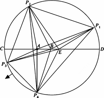
Angles are measurable through observations and were always the primary concern of the astronomers of the 1600s; even time was represented by an angle. In the derivation of his vicarious orbit, Kepler used opposition observations made with respect to the sun, so that the heliocentric longitude of Mars was directly known, because the geometry of the earth's orbit did not enter. With twelve observations of Mars at opposition at his disposal, he selected four that had a reasonably uniform distribution along the orbit, and by these he worked out a planetary model using a traditional equant and a circular orbit. The equant is the reference point at the line of apsides, around which Mars moves at a constant angular speed. But unlike previous astronomers, he allowed the equant to fall at an arbitrary place along the apsidal line. We show in fig. 1 a modified reproduction of one of the diagrams of chapter 16, where P1-P4 represent the four positions of Mars at the four oppositions, A, B, and E represent the sun, the center, and the equant, respectively, and CD is the line of apsides.
P1-P4 represent the four positions of Mars at the oppositions of 1587, 1591, 1593 and 1595. A, B and E represent the sun, the centre of the circle, and the equant, respectively. The arrow shows the direction of the vernal equinox.

At each of the four observations, both the heliocentric longitude was known (measured from A), and the angle about the equant (measured from E and called the mean anomaly) which is proportional to the time interval between the observations. The model is specified by four parameters: the eccentricity AB, the equant offset AE, the direction of the apsidal line AD, and the time when the planet was at the aphelion point D. Kepler was not able to find a geometrical solution of this problem, and he attacked it by two series of nested, wearisome iterations, by which he determined the best alignment of the sun, center, and equant with respect to orientation and distances. He describes his method of an inner iteration within the body of an outer one, as a “duplicem falsam positionem” (Kepler [Reference Kepler and Caspar1609] 1937, Vol. III, 153). First he guesses the direction of AD, which he knew fairly well but wanted to improve, together with the time of aphelion, and computed a pair of opposite angles in the quadrilateral P1P2P3P4, which should equal 180° if the four points lie on a circle. In the first trial they did not, so the direction AD is altered with a step value and the test made again. A combination of the two trials recommends a better position for AD, and the calculation is repeated. When this process has converged, Kepler calculated the triangle P2P4B to test if the center of the circle B fell on the line AE between the sun and the equant. This second process also has to be repeated by adjusting the time of aphelion, which is the same as rotating the model at a small angle around the equant E. In each case the first process has to be started again, until finally both processes succeed fairly well. The final result of these nested processes was a model that predicted the heliocentric longitude of Mars with a precision comparable with that of observations (Gingerich [1964] Reference Gingerich1993, figure 5).
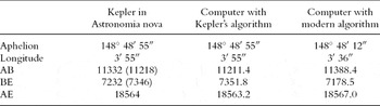
Kepler asks for sympathy from his readers because he had carried out the procedure more than 70 times. This can not be due to low efficiency of the algorithm since it takes about 9 trials to carry out Kepler's calculations, but was probably spent on redundant data differing only in the values chosen for the initial four observations (Gingerich [1973] Reference Gingerich1993), and only the final stage is printed in Astronomia nova. Table 1 presents the results from a computer implementation of Kepler's algorithm and input data, as also described in more detail by Robert Small (Small [1804] Reference Small1963, 330–338). We notice that Kepler's method and calculations are possible to reproduce on a computer. Results from an algorithm implemented by modern standards are also shown.
Orbital elements deduced from Kepler's four underlying observational sources in Astronomia nova chaps. 15–16. At the end of his computation, Kepler made an elementary numerical error (his second in this worked example), and the numbers included in parenthesis are without this fault.

However, the published worked example in Astronomia nova contains a strange error, as Kepler just forgot to add the step value to three of the four heliocentric angles at the beginning of the procedure. This initial numerical error might imply an inconstancy in the data, but with corrected input values Kepler's algorithm still performs well with almost the same solution as above (data not shown), as also noted by Owen Gingerich (Gingerich [1964] Reference Gingerich and Kraft1993). In general the procedure seems to be very robust and stable, and it is able to adjust the model parameters to fit the observation data. The method shows the existence, though not the uniqueness, of a solution (see Table 1).
Kepler's hypothesis vicaria was a preliminary success. Among the twelve oppositions, the largest disparity between his final model and the observations was only about 2′, which was the margin of observational error in the measurements themselves. This was better than the models of his predecessors. However, the assumed model later failed to give the correct distances between Mars and the sun. These relative distances can be obtained by considering the triangle Sun-Earth-Mars, obviously when they are not in opposition. By observing the latitude of Mars north and south of the plane of the ecliptic, and using some trigonometry, Kepler could determine how far Mars was from the sun. Hence, a paradox emerged: how can Mars have one required orbit according to his longitude model, and another when investigated directly according to distance? This problem ultimately forced Kepler to give up the circular orbits.
It is also of interest to note that in his Apologia pro Tychone contra Ursum (Jardine Reference Jardine1984), written at the end of 1600, Kepler compares the classical method of regula falsi by which one can obtain a solution of an equation through successive approximations, with the successive improvements of astronomical hypothesis in the quest for a better fit between observations and calculations:
In what is known as the “rule of the false,” . . . a number is sought which when handled by the prescribed rules will come to some particular value. Whatever number comes to mind is chosen and handled by the rules laid down, and if it comes to the value hoped for it is the number sought; but if it comes to less it is false. The same thing is tried out on another [number] and the two are compared, as are their deviations, and from the inspection of these things the true [number] is eventually elicited. I shall now say, using the same form of words, what in astronomical hypotheses is similar to this. Hypotheses are sought which will correspond to the motions of the heavens. The Alphonsine hypotheses are found to err, likewise the Copernican. But the skilful practitioner, having made a comparison of the two and having removed the sources of error, establishes some third [hypothesis] which avoids all error in the prediction of the motions of the heavens and in that way corrects both hypotheses. (Ibid.)Footnote 2
This “regula falsi in testing hypothesis” is applied as his very method to reach a better fit between data and model. By this approach, later described as a “rhetoric of failure” (Voelkel Reference Voelkel2001, 164), Kepler foreshadowed his own successful method (Hon Reference Hon1987).
3.2. Infinitesimal approach
Our next remark is Kepler's geometric approach in his solution of problems, using incremental micro-sectors. To illustrate Kepler's thinking on this subject, we have chosen his use of infinitesimals in his proof of the second planetary law in Epitome, book 5, part I, chaps. 3 and 4 (Kepler [1618–21] 1995, 135–143). The second law came out of his analysis of the transverse (in longum) component of motion, as seen from the sun. His first law had already been deduced as a consequence of the radial (in altum) component of motion.
His hypotheses at this stage are:
• The planetary orbits are elliptical;
• The velocity of a planet's motion transverse to its radius vector, vT, is vT = k/r, k = constant, r = radius (often called the Radius Law);
• Lines and areas can be considered as composed of increments or infinitesimal elements of the same dimension as the line or the area. We will use δ as notation.
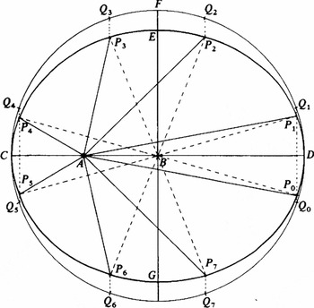
The only motion with non-constant velocity that was analyzed in physics up to this time was the motion of bodies with constant acceleration. Velocity was a difficult virtual concept in Kepler's natural philosophy, because the velocity of a planet was always changing. His theoretical analysis was done with geometry, and velocity was neither a geometrical magnitude nor a pure number. It could not be shown on a geometrical diagram of the orbit. In his proofs, Kepler instead employed increments of geometrical areas. These areas are not placed at random, but are two sectors around the symmetry lines CD and EG (see fig. 2).
A is the position of the sun and B is the center of the auxiliary circle. The planet is moving in the elliptic path P1, P2. . ., and Q1, Q2. . . is the position of a virtual planet projected on the auxiliary circle.

The circle around the ellipse is an auxiliary circle (often called the eccentric circle by astronomers) with radius a, and it is divided into equal increments, a·δβ, where we on Kepler's behalf stipulate δβ < 0.25 degrees. When it comes to numerical work it was Kepler's practice to put a = BD = 100,000 in the auxiliary circle, and the error tolerance was to ignore all fractional parts. This is the same as correcting all values to five decimal places. Within this error limit he could put 2 sin (δβ/2) = δβ, and cos (δβ/2) = 1. Accordingly, the circle arc in each division could be set equal to the corresponding chord, and the length from B perpendicular to the chord could be set equal to the radius in an auxiliary circle. Consequently areas of infinitesimal circle and ellipse segments could be approximated with infinitesimal triangles.
Following this practice, and using the geometric properties of the ellipse, Kepler found the two “area-twins” (details of the mathematics can be found in Stephenson Reference Stephenson1987, 161–165, and Davis Reference Davis2003):

Then Kepler exchanged B for the sun's center A. The sums of the areas are the same, because the heights in the “area-twins” are preserved (Kepler makes reference to one of Apollonius’ propositions).
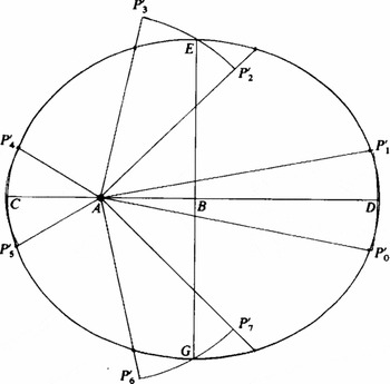
Now in order to use his Radius Law, Kepler replaces each area with a circle sector centered at A (see fig. 3). The radius of these circles is selected so that the areas are preserved.
The sun at position A, and the two particular “area-twins” used by Kepler.

Now, the sum of the heights in these two new “area-twins” is also the same (2a), but then

By the Radius Law, the time used in each of these sectors is related in the same ratio as their distances to the sun, and by the argument above, consequently also in the same ratio as their areas. So time can be represented geometrically, and he concludes (Kepler [1618–1621] 1995, 143):
Therefore the total area of the ellipse – which has been cut up at A into triangles – is distributed among the arcs in the same proportion wherein the total periodic time has been distributed among them. Therefore the single triangles are proportionally the most exact measures of their single arcs.
And on the same page he added some words to apologize for the presentation he had given in his earlier publication:
I confess that the thing is given rather obscurely there [Astronomia nova], and most of the trouble comes from the fact that there the distances are not considered as triangles, but as numbers and lines.
For Kepler the elements of time and space were infinitesimal magnitudes but never zero. The most probable interpretation of Kepler's infinitesimals in Epitome, is a kind of finite increments, which means discrete quantities smaller than a given limit. Originally they corresponded to a day, a natural step related to astronomical observations.
Kepler's approach is both geometric and numeric in nature, although the deduction of the second law is incomplete and not general. Ann Davis has shown that his method can be used to arrive at a general deduction of his law, using reasoning that lay entirely within his power (Davis Reference Davis2003). We may consider Kepler's second law to be a kind of computational technique.
3.3. Iterative approximation method for solving equations
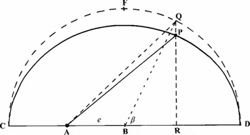
To compute areas inside the ellipse is not easy. There is no simple or exact way to find explicitly the position angle corresponding to a given time, and consequently there was no direct way to calculate the planet's position exactly from its date, as it had always been possible before Kepler. In fact it was the auxiliary circle that saved Kepler at this point (see fig. 4). One of the fundamental properties of the ellipse is the ratio-property:

A is the position of the sun and B is the center of the auxiliary circle. The planet is at P, and Q is its projection on the circle. Kepler's problem is to determine the angle β (the eccentric anomaly).

Kepler's law states that time is proportional to the ellipse area ADP. This area is composed of the triangle ARP and the segment RDP. By equation (1) the triangle is proportional to the triangle ARQ and the segment is proportional to the segment RDQ. Consequently time is proportional to the circle area ADQ which is β + e sin β. Here e is the constant AB and β the angle QBD called the eccentric anomaly. Analytically, Kepler expressed the problem by the equation

where M is the measurement used to designate time (the Mean anomaly). Kepler measured M as a fraction of the area of the full circle. The Mean anomaly is proportional to the time elapsed, and it is as a function of time that we wish to find the position of the planet P. So the important problem is to find β when M and e are given. This transcendental equation is called Kepler's equation and turned out to be a famous problem as it is fundamental in celestial dynamics (Colwell Reference Colwell1993). Kepler could only solve it in particular cases by approximations (Swerdlow Reference Swerdlow2000).
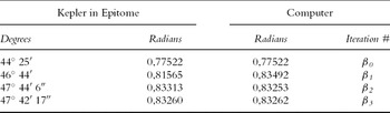
The problem was stated at the very end of Astronomia nova (Kepler [Reference Kepler and Caspar1609] Reference Kepler and Donahue1992, 600). In Epitome, book 5, part II, chap. 4 (Kepler [1618–1621] 1995, 158–59), he gives a numerical example with three iterations as shown in Table 2. The eccentricity e is determined from the area of the triangle ABF, which he says he earlier had calculated to be 11910″. Kepler had interchanged two digits here, because the preceding example six pages earlier used the number 19110″, a number which corresponds to e = 0.09265, the best estimate Kepler had for the planet Mars. Anyway, the new number will work well as a mathematical example, and determines e = 0.05774.
Kepler's numerical solution of his equation in Epitome, book 5, part II, chap. 4, compared with a simple computer iteration based on βn = M – e sin βn-1. Eccentricity e = 0.05774, and the Mean anomaly M = 50° 9′ 10″ (= 0.87533 in Radians). The convergence is quite rapid in this case.

Kepler's method can be described as a simple numerical “fixed point method,” that is, an iterative algorithm which generates a convergent sequence whose limit is the solution of the proposed problem:

He called his method to solve equations the regula positionum (rule of supposition) (Kepler [1618–1621] Reference Kepler and Wallis1953, Vol. VII, 392), probably an allusion to the classical method of regula falsi (rule of false position). But he made no closer examination of the speed of convergence or errors involved. Later, in his Tabulae Rudolphinae, Kepler solved the equation for a grid of uniformly spaced angles, which determined a set of non-uniformly spaced times. By an interpolation scheme the desired values of time could be determined, and hence no iterations were required in his Tabulae Rudolphinae at that point.
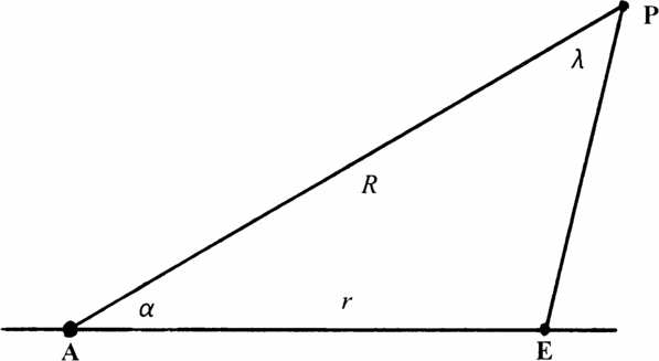
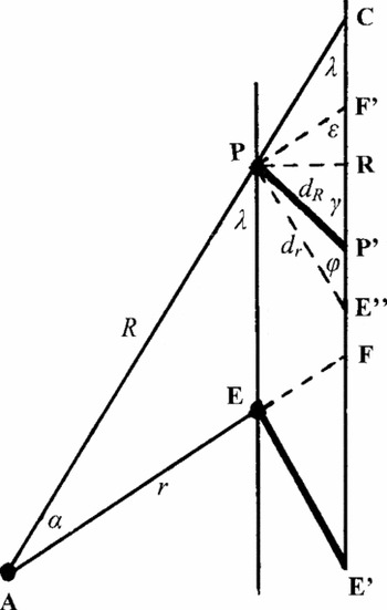
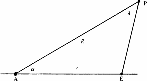
But Kepler applies similar iterative methods several times in Tabulae Rudolphinae. In chapter 9 and 22 (Kepler [1627] 1969, Vol. X, 66–69 and 144–146) he uses an iterative approach to find the angel λ between the sun (A) and the earth (E) as seen from a planet (P) (see fig. 5). Here the heliocentric angle α, and the ratio between the distances r/R, are assumed to be given, and in the triangle we have

This gives rise to the iterative procedure defined by

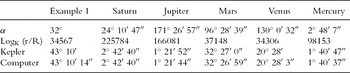
By repeating this procedure until λn ≈ λn−1, Kepler determined accurate iterative solutions of this equation for several cases, as shown in Table 3.
A is the position of the sun, E the earth, and P an outer planet.
Kepler's numerical computations of the angle λ in Tabulae Rudolphinae, chaps. 9 and 22, compared with computer solutions based on the same iterative procedure. Here the Keplerian logarithms are related to the natural logarithms by LogK(x) = ln(105/x).

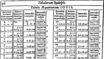
Kepler's planetary tables were completed in 1624, and printed in 1627 (see fig. 6). These Tabulae Rudolphinae made use of Kepler's logarithms and provided the means to calculate the position of any planet hundreds of years into the future or the past. In European history these tables were the third truly new set of planetary tables, following the tables of Ptolemy and Copernicus’ defenders, and they soon proved to be more accurate. Kepler designated these tables his principal astronomical result. The theory and methods he had developed in previous years were merely preparatory work to enable him to arrive at this long-awaited climax. The tables of Philip van Lansbergen (1561–1632) were the main competitor in the 1630s (Lansbergen Reference Lansbergen1632). They supported Copernican theory, but did not accept Kepler's ellipses.
Portion of one of the pages in the Tabulae Rudolphinae from 1627. This particular table provides data for predicting the position of Jupiter, and is used in converting the planet's mean anomaly (M) to eccentric anomaly (β), that is, in the solution of what was later called Kepler's transcendental equation. β runs in steps of 1° from 0 to 180°.

The Tabulae Rudolphinae were intended for general use among academics with the necessary knowledge of astronomy, and the first edition was as huge as 1,000 copies, a large number for a science book in those days. It consisted of about 40 different tables, and the reader was given around 200 “instructions for use” (praecepta) (Bialas Reference Bialas1969, 78). Instead of providing a sequence of solar and planetary positions for specified days (like modern almanacs), the Tabulae Rudolphinae were set up to apply interpolation for the calculation of solar and planetary positions for any time in the past or future. The finding of the longitude of a given planet at a given time was based on Kepler's equation and he exploited logarithms for this tabulation. The precise geocentric positions had to be worked out by combining the heliocentric positions of the planets and the earth that were calculated separately. Logarithmic tabulations were used to facilitate calculation. Originally Kepler had planned to explain in detail how he had calculated the tables. But he gave up this intention; after all it was partly fulfilled in Epitome.
3.4. Iterative computation of stationary points
From a geocentric perspective, retrograde motion was one of the major astronomical problems requiring attention. To all appearances, the planet would move in its direct order, gradually slow down and finally appear to stop (first stationary point). The planet would then appear to reverse its direction (undergo retrograde). After reversing direction the planet would again slow down and appear to stop a second time (second stationary point), reverse direction again, and continue to move in its original direction.
In fig. 7, A is the sun, P′P the daily motion of the planet, and E′E the daily motion of the earth. When E′P′ is parallel with EP, the planet will be observed as stationary from the earth. E″P is parallel with E′E and F′P is parallel with FE. PR is perpendicular to FC and PR is set to equal 1. The eccentric anomaly of the planet is assumed to be given, and the task is to find the position of the earth from where the planet will appear to be stationary.
The movement of the Earth (E′E) and a Planet (P′P) around the sun (A) at a stationary point of the orbit.

Kepler solved this task by computing the stationary angle α (angulus commutationis). Here he again applied a double iterative procedure (Kepler [1627] 1969, Vol. X, 71–73 and 161–166; Bialas Reference Bialas1970). First the angle α is assigned a start value. Then the ratio between the distances to the sun, AP/AE = R/r, and the ratio between the daily arcs, PP′/PE″ = dR/dr, may be computed. Secondly, based on the geometry of fig. 7, he executes an iterative procedure over the angle γ that can be expressed as follows:

Then let
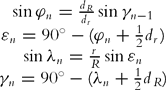
Repeat this until γn≈γn−1, and then we have

With this new value for α, both the ratio of distances and daily arcs may be corrected, and the iteration repeated all over again until the difference between α values are below a certain limit.
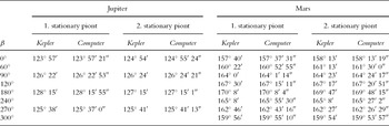
In the Tabulae Rudolphinae Kepler gave the stationary points of each planet in small inconspicuous tables consisting of four or eight eccentric anomalies of the planet. By examining the tables and Kepler's manuscripts, Volker Bialas was able to recognize the necessary initial conditions, including the time epoch, for the calculations (Bialas Reference Bialas1970). When checking the tables with a computer program based on the same algorithm as Kepler, he found almost no errors for Saturn and Jupiter, but considerable deviations for Mars and Mercury. Table 4 shows the results for Jupiter and Mars. For the main positions of Mars (β = 0, 90, 180, 270) the values are accurate within 3′, but the intermediate values may differ by more than 30′. This may indicate that the intermediate values are obtained by interpolation, and not by the wearisome iteration method.
Kepler's computations in Tabulae Rudolphinae of stationary points for Jupiter and Mars at some given values of the eccentric anomaly (β). The results are compared with computer solutions based on the same iterative procedure (Bialas Reference Bialas1970).

4. Discussion
4.1. Iterations and nested iterations
From a historical point of view it is of interest to ask who invented the iterative method of successive approximation, and how. This question at present cannot be satisfactorily answered. Hellenistic, Indian and Arab mathematicians used computations by successive approximation (Kennedy and Transue Reference Kennedy and Transue1956, 83). A trial and error procedure had been used since the time of Ptolemy to obtain parameters of circular planet models. Kepler was not the first one to explicitly use a method of approximation in which each new value is used to obtain the next value.
Heron of Alexandria (50 A.D.) already used this strategy to compute square roots (Chabert Reference Chabert1999, 202). And the Arab astronomer and mathematician Jamshid al-Kashi (ca. 1380–1429) also used iterative methods. This is found in The Treatise on the Chord and Sine that may have been unfinished at the time of his death and completed by his students. In this work al-Kashi computed sin 1° from the value of sin 3° to the same precision as he had computed π in an earlier work (Aaboe Reference Aaboe1954; Chabert Reference Chabert1999, 218). The iterative method proposed by al-Kashi was one of the great achievements in medieval algebra.
Kepler was not the first to labor with his particular equation and a numerical way of solving it. To our surprise the same equation is important in computing astronomical parallax. The Arab mathematician and astronomer Habash al-Hasib (ca. 770 – 870), who lived in Baghdad and Damascus, worked on it in connection with his eclipse theory and problems of lunar parallax. He found formulas for calculating the positions and orbits of celestial bodies that go beyond the Ptolemaic theory, and he calculated tables of sines, tangents, and standard astronomical functions (Kennedy and Transue Reference Kennedy and Transue1956). The algorithm of Habash gave a good approximation of lunar parallax after five repeating cycles of the equation. His work was probably unknown to Kepler, but our knowledge of what was known in sixteenth and seventeenth century Europe of Arabic scientific works is insufficient.
But as we have seen, Kepler's work added mathematical complexity to the astronomical models, and his innovative use of nested iterations seems to be a genuine contribution to computational mathematics. David Fabricius (1564–1617) was a clever astronomer who corresponded extensively with Kepler during the creation of Astronomia nova and challenged his methods and results. Some of this discussion was later reflected in Kepler's publications. But Fabricius was never convinced by Kepler's procedure for calculating the motion of Mars, and called it “intricate and difficult” (Voelkel Reference Voelkel2001, 200). Some of his criticism had to do with the indeterminacy in the derivation of the vicarious hypothesis, and the solution of the “transcendental” equation, since Kepler here was dealing with mathematical operations for which there were no direct procedures for solving. Kepler acknowledged the difficulty of the problems, but argued that “the outcome is wholly determined and unique” (ibid., 205). However, at the end he had to leave a rigid treatment of “transcendental” equations for a new “great Apollonius” (Kepler [Reference Kepler and Caspar1609] Reference Kepler and Donahue1992, 601), and the vicarious hypothesis for a “great Apollo” (ibid., 256), a funny announcement of the assumed fundamental character of the problems.
4.2. The reception of Kepler's work
Kepler did not get much apparent response from the leading natural philosophers of his time. Bacon, Hobbes, Pascal, Galileo, and Descartes did not notice what are today considered to be Kepler's major achievements (Applebaum Reference Applebaum1996), although they were not the mathematical astronomers to whom his work was directed.
Kepler's way of arguing in Astronomia nova and Epitome seemed initially to have confused many of his colleagues. Objections were raised against his method of summing infinitely small quantities as early as 1616 by Alexander Anderson, and in 1635 by Paul Guldin (Belyi Reference Belyi1975). In 1622 Peter Crüger, professor of mathematics at Danzig commented: “The author seems, as usual, to obscure the matter deliberately. However, I will study all these things later at leisure with my whole strength though I do not see what use this will be. These theories are based upon uncertain foundations and are mere guesswork” (Russell Reference Russell1964, 8).
Five years later, when Kepler published his accurate Tabulae Rudolphinae, Crüger became convinced of the realistic results of the theory. It was on the bases of these tables that many astronomers of the 1600s studied his other works. The tables covered all the planets, and their empirical success increased attention to Kepler's work considerably among mathematical astronomers (Russell Reference Russell1964). But some objected to the approximation and difficult calculations required by elliptical orbits, and Henry Briggs at Oxford found them unsatisfactory without giving his reasons (Applebaum Reference Applebaum1996). Modern recomputation has shown that the tables contain some errors (Bialas Reference Bialas1970), but in general they did improve planetary positions by an entire order of magnitude (Gingerich [1968] Reference Gingerich1993, 386).
Jeremiah Horrocks (ca. 1619–1641) was one of the young astronomers in England who mastered Kepler's work and promoted the new theory of planetary motions. In 1637 he developed a method of approximation necessary for finding areas of ellipse-segments which was simpler than Kepler's method, and gave results with almost the same precision (Applebaum Reference Applebaum1996). He also made adjustments to various planetary parameters, and also predicted a solar transit of Venus to take place in 1639 (Kollerstrom Reference Kollerstrom2004). Kepler's principles were gradually recognized as successful tools for predictions and discoveries, although general acceptance did not occur until Newton.
In his scientific work Kepler often had to deal with problems where a proper theory of infinitesimal calculus would have been of great help. The methods he proposed were criticized as being “ungeometrical,” imprecise, and based on tedious approximations. His astronomy teacher Michael Maestlin (1550–1631) at the University of Tübingen was generally supportive of Kepler's work, but later criticized him harshly for his use of logarithms in astronomy. In one of the introductions to logarithms Kepler commented that his mathematical colleagues had told him “it is not seemly for a professor of mathematics to be childishly pleased about any shortening of the calculations.”Footnote 3 However, Kepler did not let the deficiency stop him, as he was a tireless and ingenious approximator (Stephenson Reference Stephenson1987, 62). For example, his calculations on the planet Mars consist of nearly 900 folio pages with small handwriting. Kepler's arrangement to work within a model with a chosen level of precision constituted a vital break away from the Greek tradition. And it made it unnecessary for him to suppose that the infinitesimal interval vanished to zero, but he gave no further analysis of the error involved. It was not until Gauss (1777–1855) that a systematic study of truncation errors was begun (Goldstein Reference Goldstine1977).
4.3. The calculating machine
Kepler was in constant need of some kind of computing power. Could this be achieved in a more mechanical way? A mechanical calculator is a machine that can automatically perform arithmetical operations. In these years Wilhelm Schickard (1592–1635) was the first inventor with the necessary technical skill to design and make a pioneering mechanical calculating machine (Hammer Reference Hammer1958; Freytag-Löringhoff Reference Freytag-Löringhoff and Seck1978). Schickard was professor of Hebrew, mathematics, astronomy, and other subjects at the University of Tübingen. He was also known to be a good mechanic, and had made some of the illustrations in Kepler's books. They first met in Tübingen in 1617 and eventually knew each other well and collaborated on several occasions (Williams Reference Williams1983, 284), including on Kepler's logarithm book Chilias logarithmorum.
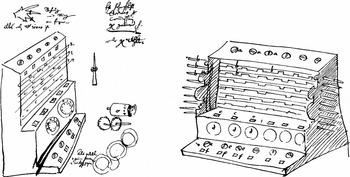
One result of these projects was that Schickard produced the first workable mechanical calculator in 1623. In devices like this, a main problem to be solved is that of recording carries and borrows resulting from additions and subtractions. Schickard solved this by employing an intricate system of mutilated and auxiliary gears. This mechanism is located in the mechanical middle section of the calculator where additions and subtractions are done (see fig. 8). In the upper part, the multiplications are done by the medieval method par gelosia, sometimes called lattice multiplication. This technique is closely related to the use of “Napier bones,” which Schickard probably knew (Freytag-Löringhoff Reference Freytag-Löringhoff and Seck1978, 305; Kistermann Reference Kistermann and Seck1995, 260). Divisions could not be done directly, but had to be performed by multiplication with the reciprocal value of the divisor. Reciprocal value tables existed for this use. In this way the calculator could be used for all contemporary types of calculations. In the bottom part of the calculator we find a manual memory where the results are stored. There are no direct connections between the three parts of the machine; the independent components are just housed in one box. Schickard informed Kepler of his mechanical calculator, and of a second copy of it, in letters written in 1623 and 1624:
What you have done by calculation I have just tried to do by way of mechanics. I have constructed a machine consisting of eleven complete and six incomplete sprocket wheels, which can calculate. . . . [It] immediately computes the given number automatically, adds, subtracts, multiplies, and divides. Surely you will beam when you see how [it] accumulates left carriers of tens and hundreds by itself or while subtracting takes something away from them. . . . I had placed an order with a local man, Johan Pfister, for the construction of a machine for you; but when half-finished, this machine, together with some other things of mine, especially several metal plates, fell victim to a fire which broke out unseen during the night. . . . I take the loss very hard, now especially, since there is no time to produce a replacement soon. (Freytag-Löringhoff Reference Freytag-Löringhoff and Seck1978, 289–290)
Schickard's drawings of his mechanical calculator (Freytag-Löringhoff Reference Freytag-Löringhoff and Seck1978, 296–97). The drawing to the left (The Stuttgart draft) was probably made for persons in the mechanical workshop. It was published by A. Georgi in 1912 (Freytag-Löringhoff Reference Freytag-Löringhoff and Seck1978, 291). To the right is the completed calculator as presented to Kepler in the letter from 1624 (The Pulkovo draft). This drawing was rediscovered by Hammer around 1935. During the time between the drawings the calculator had increased from 5 to 6 digits. Both drawings were more or less unknown until 1957 (Hammer Reference Hammer1958).

Schickard's calculator could use only six digits because of mechanical limitations in the wheels that were in production at this time. When the numbers became larger, Schickard had provided a small bell which rang each time an overflow occurred. A set of brass rings could be slipped over the fingers of the operator to count the overflow (see the top of fig. 8).
In a letter to Philipp von Hessen written in 1623, Kepler mentioned the need for seven or at most eight digits; five would not be enough for the trigonometric values (Kistermann, Reference Kistermann and Seck1995, 254). Large numbers had to be multiplied by splitting them into smaller portions, treating them separately, and adding up the partial sums. Such a system could have worked well in practice with the precision required by Kepler (Kistermann Reference Kistermann2001). But judging from the letters, nothing indicates that the calculator was used in realistic astronomical calculations and work. It seems to have been a prototype for testing. It was in some sense more advanced than Pascal's mechanical calculator, which came about 20 years later, and could perform only linear operations like addition and subtraction. Schickard's design was a true three-function calculator with six-digit accumulator.
Two years after Kepler died, Schickard published a pamphlet giving a brief outline of Kepler's astronomical theory (Russell Reference Russell1964, 11). But the calculator is not mentioned – the logarithms and mathematical tables had established themselves as mainstream in computational science for the coming 300 years. The prototype called the Calculating Clock was forgotten. No trace of it has been found in museums and scientific collections. It turned out to be a dead end, although to our knowledge, it was the first invention of such a device. From Schickard's diagrams it has been possible to reconstruct a complete and functional calculating machine (Freytag-Löringhoff Reference Freytag-Löringhoff and Seck1978; Kistermann Reference Kistermann2001).
4.4. Relation to the Newton-Raphson method
Later Newton (1642–1727) was the first to show novel interest in Kepler's equation, and he proposed three solutions of it through the various editions of the Principia and in other writings (Colwell Reference Colwell1993, 51). In the first edition of Principia (1687), Book I, prop. XXXI, Newton demonstrates how “to find the place of a body moving in a given ellipse at any assigned time.” In his comments on this difficult problem, he proposed a geometric solution, hard to follow. In the later editions he suspended this impractical method, and introduced an iterative procedure. This description is Newton's first publication of what we today know as the “Newton-Raphson method” (Whiteside Reference Whiteside1974, 316–319).
So the general “Newton-Raphson” iterative method has a historic relation to the Kepler problem. In nearly every decade since then there have appeared papers devoted to Kepler's Equation and its solution (Colwell Reference Colwell1993), and mathematics like the cycloid and the Bessel functions were introduced. Many eminent mathematicians have worked on it, including Lagrange (1771), Gauss (1809), Bessel (1816–17), and Laplace (1823) (Belyi Reference Belyi1975). Kepler's own iterative solution was applied by Leonard Euler (1707–1783) and others. Euler was aware that the method is slow when e is close to 1, and he had to make huge numerical calculations. But the problem never had the appeal of Fermat's great theorem, or the depth and intractability of the many-body problem. With modern calculators and computer software, there are no limits on finding quick solutions of great accuracy. Excel was used to prepare Tables 2 and 3.
5. Conclusions
Several methodological innovations were required by the new astronomy. Kepler mainly justified them as truth-linked, by requiring converging support from both the theoretical and the empirical hypothesis (Martens Reference Martens2000, 111). In this way he mapped the mathematical onto the physical, and he became an active promoter of the new art of computing. His background in the traditional principles of Greek mathematics and physics was in definite areas in great contrast to his excitement for reforms in natural philosophy, and his input to the upcoming synthesis was to transcend the classical use of only geometrical methods as appropriate in astronomy. His main improvements within computational mathematics were in the area of numerical analysis. In this paper we have traced iterative methods as a common theme in three of his major astronomical publications. Kepler posed important problems, allowed approximations, used increments, iterations, nested iterations, and prepared precompiled mathematical lookup tables for practical use. In effect he was also dealing with the summation of an unbounded number of infinitesimals. This “atomistic” approach to the solution of a difficult mathematical problem represents an important step in the early history of numerical analysis, which offered much of value to his successors, although it lacked a firm logical foundation.
Kepler's astronomical research was a stimulating laboratory for the early development of numerical analysis. His iterative methods were also inspired by the classical method of regula falsi. The problem at hand could not be solved by formal geometry, only by approximations – that is by an iterative trial-and-error procedure which had to be continued until all the quantities in the equation fitted together tolerably well. His treatment was not rigorous, although it was mathematical and numerically robust. Kepler's contributions were mainly based on intuition, with a strong metaphysical flavor, and embedded concepts of great importance for the further development of mathematics. His use of nested iterations was new within natural philosophy, and the “Kepler equation” was one of the first transcendental equations to be studied. The equation was probably new to Kepler, but is today known to have been studied by Arab astronomers in a different context. We would describe his iterative solution as a numerical “fixed point method.” Later Newton developed a technique called the “Newton-Raphson method” to solve the same equation.
Schickard's mechanical calculator was designed at the turning point in the development of computational mathematics and technology. But the innovative calculator that once operated in Tübingen never came into regular use. However, it is of interest to note that the first calculator of this type was created in an explicit scientific context. Mechanical computing naturally belonged to the visions of pioneering work in modern science, although Schickard's design of the six-digit calculator was forgotten. But Schickard and Kepler were genuine scientific innovators, and not just pale predecessors of Pascal and Newton.
When Kepler gave the new physical astronomy both a mechanistic treatment and a mathematical representation, an important and vital new relationship between mathematics and natural philosophy was established. A great need for computing power was one of the problems at the time when the new sciences were founded. And in this context Newton and Leibniz's mathematical analysis can be seen as an elegant, but abstract, by-pass operation for the problem of getting lost in calculations. So when we are introducing numerical techniques on computers in our mathematical lessons, we are close to the genetic approach, well rooted in both early history of mathematics and in modern scientific practice.
Acknowledgement
The author thanks Jørgen Albretsen at Aalborg University for his implementation of the hypothesis vicaria, and for compiling Table 1.