2 Problem setting

The Boussinesq equations, with constant rotation and stable stratification are:

(2.1) $$\begin{eqnarray}\displaystyle & \displaystyle \unicode[STIX]{x2202}_{t}\boldsymbol{u}+\unicode[STIX]{x1D735}p+\boldsymbol{u}\boldsymbol{\cdot }\unicode[STIX]{x1D735}\boldsymbol{u}=f\boldsymbol{u}\times \hat{z}-N\unicode[STIX]{x1D703}\hat{z}+\unicode[STIX]{x1D708}\unicode[STIX]{x1D6FF}\boldsymbol{u}, & \displaystyle\end{eqnarray}$$

(2.2) $$\begin{eqnarray}\displaystyle & \displaystyle \unicode[STIX]{x2202}_{t}\unicode[STIX]{x1D703}+\boldsymbol{u}\boldsymbol{\cdot }\unicode[STIX]{x1D735}\unicode[STIX]{x1D703}=Nw+\unicode[STIX]{x1D705}\unicode[STIX]{x1D6FF}\unicode[STIX]{x1D703}, & \displaystyle\end{eqnarray}$$

with $\boldsymbol{u}=(u,v,w)$ the incompressible velocity field, $\unicode[STIX]{x1D735}\boldsymbol{\cdot }\boldsymbol{u}=0$ and $p$ the pressure; $\unicode[STIX]{x1D703}$ represents temperature (or density) fluctuations, in units of a velocity, since we want to stress the energetics of these flows. These fluctuations are superimposed on a stably stratified background with a linear vertical profile $\bar{\unicode[STIX]{x1D703}}(z)=\unicode[STIX]{x1D703}_{0}+z\unicode[STIX]{x2202}_{z}\bar{\unicode[STIX]{x1D703}},~\unicode[STIX]{x2202}_{z}\bar{\unicode[STIX]{x1D703}}<0$ . Introducing the buoyancy $b=N\unicode[STIX]{x1D703}$ (note the choice of sign), with point-wise vertical flux $b(\boldsymbol{x})w(\boldsymbol{x})$ , as well as the integrated buoyancy flux

(2.3) $$\begin{eqnarray}\displaystyle & \displaystyle B_{f}=\langle N\unicode[STIX]{x1D703}w\rangle , & \displaystyle\end{eqnarray}$$

one recovers the more standard form of the equations in terms of $b$ . $N=\sqrt{-(g/\unicode[STIX]{x1D703}_{0})\unicode[STIX]{x2202}_{z}\bar{\unicode[STIX]{x1D703}}}$ is the Brunt–Väisälä frequency, and $\unicode[STIX]{x1D708}=\unicode[STIX]{x1D705}$ are the viscosity and thermal diffusivity. The Boussinesq equations are integrated using direct numerical simulations. A cubic box of $n_{p}^{3}=1024^{3}$ points is used for 56 runs (see table 1), with a linear dimension $L_{box}=2\unicode[STIX]{x03C0}$ , resulting in wavenumbers in the range $1\leqslant k\leqslant k_{M}=n_{p}/3$ using a standard 2/3 dealiasing rule. All length scales defined below are thus expressed in terms of the fundamental length $L_{box}=2\unicode[STIX]{x03C0}$ , which of course can be rescaled to the physical problem when necessary. Another smaller set of runs, at lower resolutions, is also analysed (see table 2). The pseudo-spectral code we use, GHOST (Geophysical High-Order Suite for Turbulence), is parallelized in a hybrid fashion with both MPI and Open-MP (Mininni et al. Reference Mininni, Rosenberg, Reddy and Pouquet2011) and demonstrates scalability to in excess of 130 000 cores. It includes many solvers for fluid and magnetohydrodynamic turbulence, and it now also has the capability to simulate a non-cubic geometry (Oks, Mininni & Pouquet Reference Oks, Mininni and Pouquet2018). GHOST has been tested in the purely stratified case against the numerical results of Kimura & Herring (Reference Kimura and Herring1996) for random initial conditions, and of Riley & deBruynKops (Reference Riley and deBruynKops2003) for the Taylor–Green flow.

Table 1.

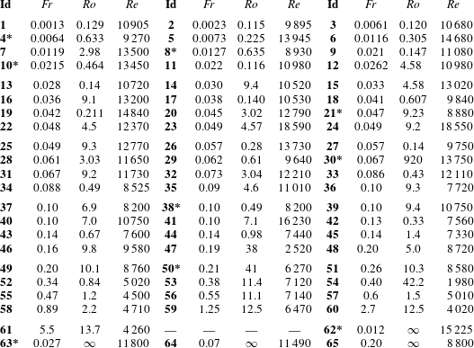
Nomenclature of the runs performed on grids of $1024^{3}$ points, with Id, $Fr,Ro$ and $Re$ the identification of runs and their Froude, Rossby and Reynolds numbers, the runs being ordered by $Fr$ (see also Rosenberg et al. (Reference Rosenberg, Marino, Herbert and Pouquet2016)). Initial conditions are centred on the large scales and are isotropic for the velocity field, and zero for the temperature. Runs 62 to 65 are purely stratified. Note that the 9 runs marked with a star are not included in the present study (see § 3.1); they are specifically runs $\text{Id}=4$ , 8, 10, 21, 30, 38, 50, 62 and 63.

For the runs of table 1, the potential energy is initially zero, and initial conditions for the initial velocity, with a non-zero vertical component, are isotropic, random and centred on the large scales ( $2\unicode[STIX]{x03C0}/L_{0}=k_{0}=2.5$ ); energies are defined as:

(2.4a-c ) $$\begin{eqnarray}\displaystyle E_{V}=\frac{1}{2}\int \Vert \boldsymbol{u}(\boldsymbol{x})\Vert ^{2}\,\text{d}^{3}\boldsymbol{x},\quad E_{P}=\frac{1}{2}\int |\unicode[STIX]{x1D703}(\boldsymbol{x})|^{2}\,\text{d}^{3}\boldsymbol{x},\quad E_{T}=E_{V}+E_{P}, & & \displaystyle\end{eqnarray}$$

$E_{T}$ being the total energy. They can also be written in terms of their respective isotropic Fourier spectra, with $\int E_{V,P}(k)\,\text{d}k=E_{V,P}$ . Similarly, the kinetic, potential and total rates of energy dissipation are:

(2.5a-c ) $$\begin{eqnarray}\displaystyle \unicode[STIX]{x1D716}_{V}=\unicode[STIX]{x1D708}\int \Vert \unicode[STIX]{x1D74E}(\boldsymbol{x})\Vert ^{2}\,\text{d}^{3}\boldsymbol{x},\quad \unicode[STIX]{x1D716}_{P}=\unicode[STIX]{x1D705}\int \Vert \unicode[STIX]{x1D735}\unicode[STIX]{x1D703}(\boldsymbol{x})\Vert ^{2}\,\text{d}^{3}\boldsymbol{x},\quad \unicode[STIX]{x1D716}_{T}=\unicode[STIX]{x1D716}_{V}+\unicode[STIX]{x1D716}_{P}. & & \displaystyle\end{eqnarray}$$

Note that $\unicode[STIX]{x1D716}_{V}$ can be measured relative to its dimensional evaluation of kinetic energy dissipation for a fully turbulent flow as:

(2.6a-d ) $$\begin{eqnarray}\unicode[STIX]{x1D6FD}\equiv \unicode[STIX]{x1D716}_{V}/\unicode[STIX]{x1D716}_{D},\quad \unicode[STIX]{x1D716}_{D}\equiv u_{rms}^{3}/L_{int},\quad u_{rms}=[\langle |\boldsymbol{u}|^{2}\rangle ]^{1/2},\quad L_{int}=2\unicode[STIX]{x03C0}{\displaystyle \frac{\displaystyle \int [E_{V}(k)/k]\,\text{d}k}{\displaystyle \int E_{V}(k)\,\text{d}k}},\end{eqnarray}$$

where $L_{int}$ is the integral scale (Monin & Yaglom Reference Monin and Yaglom1979). $\unicode[STIX]{x1D6FD}$ is a key parameter of the phenomenological and theoretical understanding of the interactions between waves and turbulence (Zakharov, L’vov & Falkovich Reference Zakharov, L’vov and Falkovich1992), as also discussed in § 3.3.

The governing dimensionless parameters of the Boussinesq equations measure the strength of nonlinear interactions relative to dissipation, rotation and stratification; they are the Reynolds ( $Re$ ), Rossby ( $Ro$ ) and Froude ( $Fr$ ) numbers, defined as usual as:

(2.7a-c ) $$\begin{eqnarray}\displaystyle Re=\frac{u_{rms}L_{int}}{\unicode[STIX]{x1D708}},\quad Ro=\frac{u_{rms}}{fL_{int}},\quad Fr=\frac{u_{rms}}{NL_{int}}, & & \displaystyle\end{eqnarray}$$

with the Prandtl number $Pr=\unicode[STIX]{x1D708}/\unicode[STIX]{x1D705}$ taken equal to unity. The buoyancy Reynolds number, the Richardson number and the turbulent intensity are defined as:

(2.8a-c ) $$\begin{eqnarray}\displaystyle {\mathcal{R}}_{B}\equiv ReFr^{2},\quad Ri\equiv [N/\langle \unicode[STIX]{x2202}_{z}u_{\bot }\rangle ]^{2},\quad {\mathcal{R}}_{I}\equiv \unicode[STIX]{x1D716}_{V}/[\unicode[STIX]{x1D708}N^{2}]. & & \displaystyle\end{eqnarray}$$

$Ri$ is based on a shear time computed on vertical gradients of the horizontal wind, namely $\unicode[STIX]{x1D70F}_{shear}=[\langle \unicode[STIX]{x2202}_{z}u_{\bot }\rangle ]^{-1}$ . All these parameters are discussed further in §§ A.1 and A.2. In the presence of stratification, a variety of length scales can be relevant (Thorpe Reference Thorpe1987; Mater & Venayagamoorthy Reference Mater and Venayagamoorthy2014), e.g.

(2.9a-c ) $$\begin{eqnarray}\displaystyle L_{B}=2\unicode[STIX]{x03C0}\sqrt{E_{V}}/N,\quad L_{Ell}=2\unicode[STIX]{x03C0}\sqrt{E_{P}}/N,\quad \ell _{Oz}=2\unicode[STIX]{x03C0}\sqrt{\unicode[STIX]{x1D716}_{V}/N^{3}}, & & \displaystyle\end{eqnarray}$$

or the buoyancy, Ellison and Ozmidov scales. In purely stratified flows, $L_{B}$ is the scale for which the vertical Froude number becomes of order one (Billant & Chomaz Reference Billant and Chomaz2001); it measures the thickness of the vertical layers. On the other hand, the Ellison scale corresponds to the vertical distance travelled by a particle of fluid before being completely mixed, and it is thought to be significantly smaller than the integral scale in strongly stratified flows, as we shall show later (see figure 6 b). $L_{B}$ and $L_{Ell}$ vary as $1/N$ , but differ by a field amplitude ratio, $\sqrt{E_{V}/E_{P}}$ . Finally, the Ozmidov scale is the scale beyond which isotropy is thought to be recovered together with a classical Kolmogorov range.

Table 2.

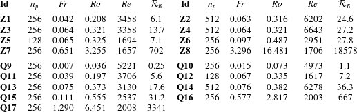
Parameters for two other sets of DNS identified by Id and ordered, for each set, by their Froude number $Fr$ , with $Ro$ and $Re$ the Rossby and Reynolds numbers computed at the time of maximum of enstrophy for each run. ${\mathcal{R}}_{B}=ReFr^{2}$ , and $n_{p}^{3}$ is the total number of grid points for each run. In runs $\boldsymbol{Z}\boldsymbol{x}$ , $x=[1,8]$ , the initial conditions are large-scale isotropic and random for the velocity field, and zero for the temperature as for the runs of table 1, whereas in the $\boldsymbol{Q}\boldsymbol{x}$ runs, $x=[9,17]$ , initial conditions are in geostrophic balance for velocity and temperature fluctuations. For both sets, $N/f\approx 5$ , a value close to what is found in the ocean.

3 Global behaviour and scaling

3.1 Overview of the runs

Runs with an emphasis on realistic parameters for the mesosphere and lower thermosphere, and which overlap with the present data base, were investigated for the energy partition between waves and slow modes and the link with kinetic–potential energy exchanges in Marino et al. (Reference Marino, Rosenberg, Herbert and Pouquet2015b ), as well as for parametric characteristic time scale variations in Rosenberg et al. (Reference Rosenberg, Marino, Herbert and Pouquet2016) (see also Rosenberg et al. Reference Rosenberg, Marino, Herbert and Pouquet2017). Here, the runs on grids of $1024^{3}$ points cover the following parameter ranges (see table 1): $0.11\leqslant Ro\leqslant 41$ , $1985\leqslant Re\leqslant 18\,590$ , $0.001\leqslant Fr\leqslant 5.5$ , $0.02<{\mathcal{R}}_{B}<1.2\times 10^{5}$ and $2.47\leqslant N/f\leqslant 312$ . Two purely stratified runs are included as well. Note that, even though the ratio in values of Reynolds numbers across all these runs is close to ten, most runs are within a factor ${\approx}4$ of each other in $Re$ , with as high a value as can be realized on the chosen grid, thus breaking large-scale balance toward isotropization, as studied already in Herring (Reference Herring1980) using a closure model of turbulence (see Pumir, Xu & Siggia (Reference Pumir, Xu and Siggia2016), Iyer, Sreenivasan & Yeung (Reference Iyer, Sreenivasan and Yeung2017) and Rubinstein, Clark & Kurien (Reference Rubinstein, Clark and Kurien2017) for recent references).

Two other small series of runs at lower resolutions have been performed (see table 2). The first study ( $\boldsymbol{Q}$ runs) is focused on the role of initial conditions, taking now geostrophically balanced fields at $t=0$ , which should radiate waves much less initially. The second small set of ( $\boldsymbol{Z}$ ) runs deals with the variation of effective dissipation $\unicode[STIX]{x1D6FD}$ defined in (2.6) with Reynolds number at fixed $N/f=5$ , with $Re$ varying by a factor in excess of 10, between $1650$ and $18\,590$ , when including runs of table 1.

All statistics are computed dynamically around the peak of dissipation, when the flow is most developed and starts its self-similar temporal decay. This is in contrast to what is done in Stretch et al. (Reference Stretch, Rottman, Venayagamoorthy, Nomura and Rehmann2010), where the data for mixing are taken when more than 90 % of the energy has dissipated, after approximately ten turnover times. Specifically, our data are averaged on a number of outputs around the peak of enstrophy, covering a relative variation in the amplitude of enstrophy of ${\approx}2.5\,\%$ . This results in using of the order of 18 outputs on average for each run, with no more than 49 and no fewer than 6; the physical time interval on which these averages were performed is of the order of a fraction of a turnover time. We find that $u_{rms}$ and $L_{int}$ do not vary much across the first large parametric study, from 0.66 to 0.89 for the former, and from 1.39 to 2.78 for the latter. Note that some of the runs tabulated in Rosenberg et al. (Reference Rosenberg, Marino, Herbert and Pouquet2016) have been removed from the data set in table 1, which has been reduced from 65 to 56 runs. This is because of various factors: archiving issues in view of the large data base that was created several years ago, or because the variation of enstrophy at peak was insufficient to satisfy the averaging criterion, or because some of the data files were corrupted.

The accuracy of the computations is quantified through the ratio of the maximum to the Kolmogorov dissipation wavenumber, $k_{M}/k_{\unicode[STIX]{x1D702}}$ , with $k_{\unicode[STIX]{x1D702}}=[\unicode[STIX]{x1D716}_{V}/\unicode[STIX]{x1D708}^{3}]^{1/4}$ ; this is done under the assumption that the small scales have recovered a Kolmogorov spectrum, i.e. that the Ozmidov length scale is resolved, or for ${\mathcal{R}}_{B}\geqslant 1$ , which is the case for the majority of our runs. For all flows of table 1, we have $0.39\leqslant k_{\unicode[STIX]{x1D702}}/k_{M}\leqslant 1.3$ , with approximately 17 % slightly under-resolved runs which all have $N/f\geqslant 10$ . We have also checked that the overall shape of the curves plotted in the figures did not depend on the resolution.

Strong activity develops at small scales, with layer destabilization, as found as well by a number of authors in the purely stratified case. An example of such structures is given in the visualizations found in Rosenberg et al. (Reference Rosenberg, Pouquet, Marino and Mininni2015) for a flow which corresponds rather closely to some of the runs computed in this data base (specifically, runs $\text{Id}=11$ , 19, 33 and 43), but done on a grid of $4096^{3}$ points, allowing for a substantially higher Reynolds number. Prominent in this flow with $N/f=4.95$ , $Fr\approx 0.0242$ , $Re\approx 54\,000$ , is the juxtaposition of large-scale eddies and an intense vortical activity at their rims in what can be called vortex lanes. Such a complex small-scale flow corresponds to local overturning instabilities, with local Richardson numbers well below 0.25 for a substantial portion of the flow (see e.g. figures 10 and 11 in Rosenberg et al. (Reference Rosenberg, Pouquet, Marino and Mininni2015)).

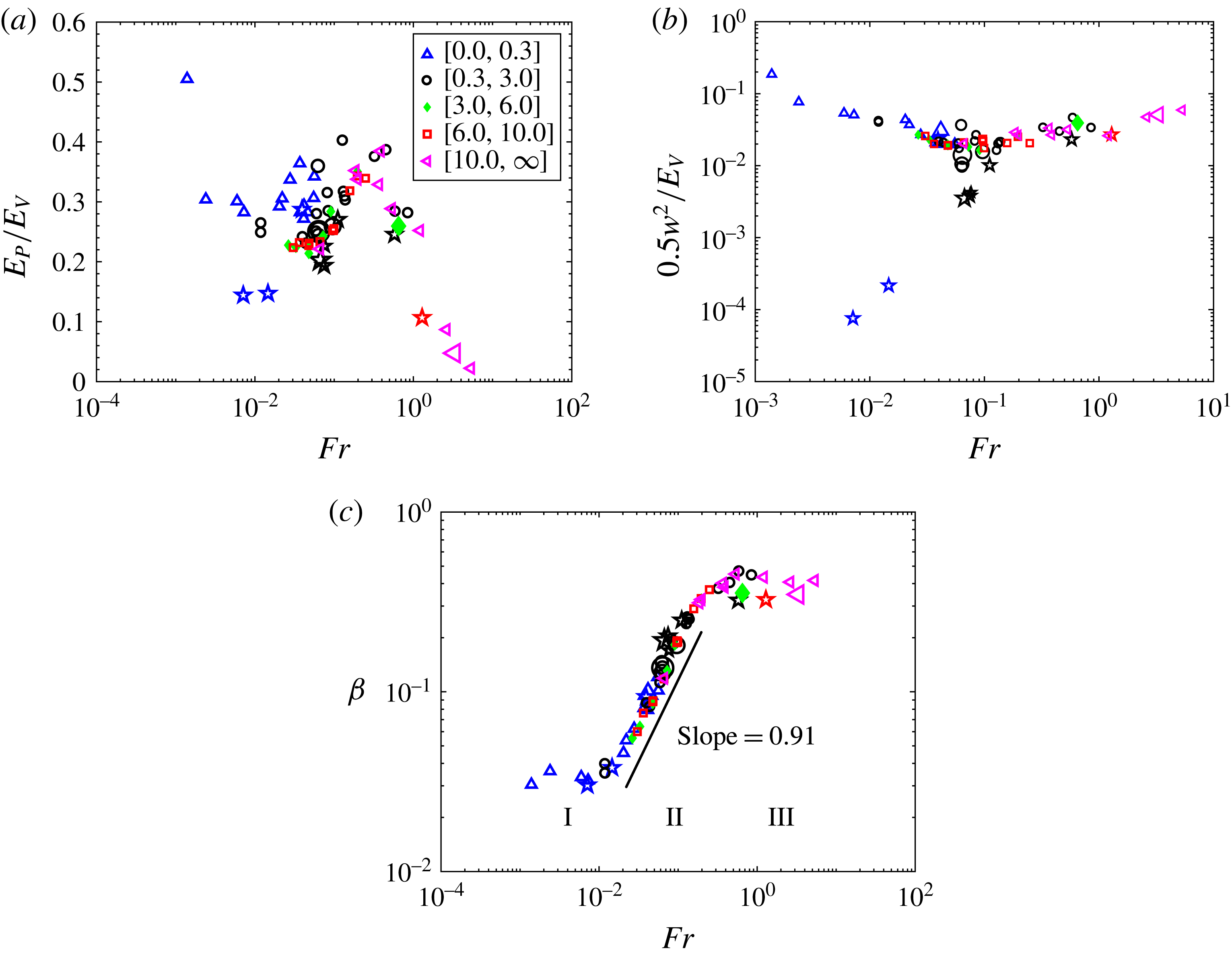
In all the figures in the present work, different symbols are used for different binning, mainly in Rossby number; stars/asterisks are used for runs with QG initial conditions (ICs), whereas the hollow shapes are always for the $\unicode[STIX]{x1D703}(t=0)=0$ ICs. Furthermore, the sizes of all symbols refer to the resolution and Reynolds number (see caption of figure 1).

Figure 1.

Variation with Froude number of the ratio of potential to kinetic energy (a), of vertical to kinetic energy (b) and of the rate of kinetic energy dissipation compared to its dimensional evaluation, $\unicode[STIX]{x1D6FD}=\unicode[STIX]{x1D716}_{V}/\unicode[STIX]{x1D716}_{D}$ (c). Colours/symbols indicate binning in Rossby number for all runs: blue triangles for $0<Ro\leqslant 0.3$ , black circles for $0.3<Ro\leqslant 2.9$ , filled green diamonds for $2.9<Ro\leqslant 6.0$ , red squares for $6.0<Ro\leqslant 10.0$ and magenta inverted triangles for $Ro>10$ (see inset). The runs of table 2 are indicated either by a star for those with quasi-geostrophic initial conditions ( $Q$ runs), or by a hollow symbol for the runs with $\unicode[STIX]{x1D703}(t=0)=0$ ; their relative size is proportional to viscosity, thus inversely proportional to $Re$ and to numerical resolution. We define the three dynamical regimes as: I for strong waves ( $Fr\lesssim 0.01$ ), II for eddy–wave interactions ( $0.01\lesssim Fr\lesssim 0.2$ ) and III for strong stratified turbulence ( $Fr\gtrsim 0.2$ ), as indicated in (c); note the quasi-linear scaling of $\unicode[STIX]{x1D6FD}$ with $Fr$ in regime II, namely $\unicode[STIX]{x1D6FD}\sim Fr^{0.91}$ .

3.2 Energy ratios

We show in figure 1 the variation of central energetic quantities, as a function of Froude number, with binning in Rossby number. The widths of the bins are chosen so as to have approximately the same number of data points in each bin, as for all other figures. The energy ratio $r_{E}\equiv E_{P}/E_{V}$ (left) varies roughly between 0.2 and 0.4, as long as the velocity and temperature remain coupled through buoyancy, i.e. for $Fr<1$ . At high $Fr$ , $E_{P}/E_{V}$ becomes negligible since the velocity is no longer constrained effectively by the waves and we have a quasi-passive scalar regime with $\unicode[STIX]{x1D703}(t=0)=0$ for most of the runs. The scaling in $Fr^{-2}$ at high $Fr$ , as advocated for oceanic turbulence in Wells, Cenedese & Caulfield (Reference Wells, Cenedese and Caulfield2010) (see also Maffioli, Brethouwer & Lindborg (Reference Maffioli, Brethouwer and Lindborg2016) for purely stratified flows), may be present as well, although we have a scarcity of points in that domain. We thus conclude that in the intermediate regime of wave–vortex interactions:

(3.1) $$\begin{eqnarray}\displaystyle & \displaystyle \unicode[STIX]{x1D703}_{rms}\sim u_{rms}. & \displaystyle\end{eqnarray}$$

The result $r_{E}\approx 1$ from below (see also Mater, Schaad & Venayagamoorthy (Reference Mater, Schaad and Venayagamoorthy2013)) is compatible with the experimental, observational and numerical data compiled in Zilitinkevich et al. (Reference Zilitinkevich, Elperin, Kleeorin, Rogachevskii, Esau, Mauritsen and Miles2008). We also find $\unicode[STIX]{x1D716}_{P}/\unicode[STIX]{x1D716}_{V}\approx 1/3$ , as measured in the stratosphere (Lindborg Reference Lindborg2006). In fact, such a quasi-equipartition of energy is present in a large range of wavenumbers, as shown in Marino et al. (Reference Marino, Rosenberg, Herbert and Pouquet2015b ) in the forced case. It immediately implies that the Ellison scale $L_{Ell}$ goes as $L_{int}Fr$ , for which in fact the scaling is excellent (see figure 6 b below), and that $L_{Ell}\sim L_{B}\sim u_{rms}/N$ . Note also that a pattern is discernible in $E_{P}/E_{V}$ with, on average, higher relative vertical velocity and higher relative potential energy at low Rossby number. As a function of Reynolds number, $r_{E}$ decreases on average for $Re$ larger than ${\approx}10^{4}$ , because of the initial conditions (not shown).

The ratio of vertical to total kinetic energy $\langle w^{2}/2\rangle /E_{V}$ is given in figure 1(b). At low $Fr,{\mathcal{R}}_{B}$ , with weak nonlinear mode coupling, its high value for the runs of table 1 is due to initial conditions, taken with a rough equipartition between velocity modes in all directions, in order to let anisotropy develop dynamically. A similar reduction in vertical velocity for rapidly rotating flows in the absence of stratification was observed in laboratory experiments (van Bokhoven et al. Reference van Bokhoven, Clercx, van Heijst and Trieling2009), together with a weaker dissipation. In an intermediate range of parameters, around $Fr\approx 0.1$ , there is a small plateau, the stratification being strong enough to prevent most of the vertical motions; so,

(3.2) $$\begin{eqnarray}\displaystyle & \displaystyle w_{rms}\lessapprox u_{rms}. & \displaystyle\end{eqnarray}$$

As turbulence strengthens with increasing $Fr$ , vertical motions develop slowly after that plateau, with an approximate scaling $\langle w^{2}\rangle \sim \langle u_{\bot }^{2}\rangle Fr^{1/4}$ . The origin of such a weak scaling is not clear, and no scaling is found in terms of $N/f$ . We recall here that the vertical velocity $w\hat{e}_{z}$ is also a direct measure of wave activity since, in a wave–vortex decomposition, as performed e.g. in Bartello (Reference Bartello1995), Herbert et al. (Reference Herbert, Marino, Pouquet and Rosenberg2016), vortical modes have vanishing $w$ . The presence of rotation facilitates vertical motions in the form of upward propagating inertial waves along Taylor columns that would form if there was no stratification, as clearly observed, including when the small scales develop strong vorticity (Davidson, Staplehurst & Dalziel Reference Davidson, Staplehurst and Dalziel2006; Mininni, Rosenberg & Pouquet Reference Mininni, Rosenberg and Pouquet2012): the vertical velocity is leaving a trace of the influence of rotation on the system and its increase is consistent with a wave–vortex analysis. The scaling in (3.2) may seem unexpected. Dimensional analysis using incompressibility at large scale would predict $w_{rms}/u_{rms}\sim Fr$ , ruled out by the data with isotropic ICs, but in agreement with the data with QG initial conditions at low Froude numbers, with this energy ratio reaching the value obtained with the isotropic ICs for $Fr\approx 0.1$ . We know that strong vertical velocities develop for intermediate $Fr$ when the buoyancy and nonlinear terms balance each other, leading to a ‘saturation’ vertical energy spectrum $E_{\Vert }\sim N^{2}k_{\Vert }^{-3}$ . The model developed in Rorai, Mininni & Pouquet (Reference Rorai, Mininni and Pouquet2014), adding the buoyancy flux to a Vieillefosse description of intermittency for FDT, leads to $E_{\Vert }\approx E_{P}\approx E_{V}$ under the hypothesis that the characteristic vertical scale is the buoyancy scale. In these intermittent regions identified by low Richardson numbers, high vertical velocities appear, due to strong turbulent stirring leading to overturning of layers. Note that it is argued in Maffioli & Davidson (Reference Maffioli and Davidson2016) that gradients are much larger in the vertical, or that $w$ is really at small scale. Thus, these authors advocate $\langle w^{2}\rangle \sim \unicode[STIX]{x1D716}_{V}/N$ . With $\unicode[STIX]{x1D716}_{V}\sim \unicode[STIX]{x1D716}_{D}Fr$ (see § 3.3 below), this leads again to $w/u_{\bot }\sim Fr$ . On the other hand, in their paper, $\unicode[STIX]{x1D6FD}$ is viewed as a constant denoted $A_{k}<1$ , independent of dimensionless parameters, so their estimate is rather $w/u_{\bot }\sim Fr^{1/2}$ , unlike our data at high $Fr$ .

3.3 Effective versus dimensional dissipation and the three regimes of RST

The dissipation efficiency of rotating stratified flows $\unicode[STIX]{x1D6FD}$ is shown in figure 1(c) as a function of $Fr$ ; it clearly displays three regimes. For small $Fr$ up to $Fr\approx 0.01$ , $\unicode[STIX]{x1D716}_{V}$ is low and constant. Similar low dissipation efficiency, of the order of a few per cent, is obtained for runs corresponding to the upper troposphere and lower stratosphere region, with low Froude numbers, as analysed for example in Paoli et al. (Reference Paoli, Thouron, Escobar, Picot and Cariolle2014) using a sub-grid model. We find that, above $Fr\approx 0.01$ , $\unicode[STIX]{x1D6FD}$ grows quasi-linearly with $Fr$ , with a least-square fit giving a slope of 0.91 after which $\unicode[STIX]{x1D6FD}$ saturates, for $Fr\gtrsim 0.2$ . Thus,

(3.3) $$\begin{eqnarray}\displaystyle & \displaystyle \unicode[STIX]{x1D6FD}=\unicode[STIX]{x1D716}_{V}/\unicode[STIX]{x1D716}_{D}\sim Fr\quad [\text{Intermediate regime, II}], & \displaystyle\end{eqnarray}$$

thereby defining the three dynamical regimes of RST, namely I, II and III, ordered by increasing $Fr$ . Such a scaling is also found when examining the small-scale energy flux in the forced case in the presence of an inverse cascade (Marino, Pouquet & Rosenberg Reference Marino, Pouquet and Rosenberg2015a ). $\unicode[STIX]{x1D6FD}$ saturates at a value close to unity for highly turbulent flows at higher Froude numbers, as found as well in Maffioli & Davidson (Reference Maffioli and Davidson2016), although their values at peak of enstrophy are a bit higher. This may be related to the fact that they compute in boxes of small aspect ratio, between $1/4$ and $1/6$ , a geometry that can favour vertical gradients and shear, and which can lead to a more active turbulence, as found in Oks et al. (Reference Oks, Mininni and Pouquet2018). When the turbulence strengthens, so does the direct energy cascade through baroclinic instability, frontogenesis and nonlinear coupling of eddies (McWilliams Reference McWilliams2016). It should finally be noted that we do not expect actual transitional values of $\unicode[STIX]{x1D6FD}$ , between regimes I and II, and II and III, to be similar for similar control parameters in different flow geometries, but we do expect the scaling $\unicode[STIX]{x1D6FD}\sim Fr$ to hold, as shown here contrasting isotropic versus QG initial conditions (see also the dimensional argument in the appendix indicating how the transfer time to small scales is moderated by the stratification).

Figure 2.

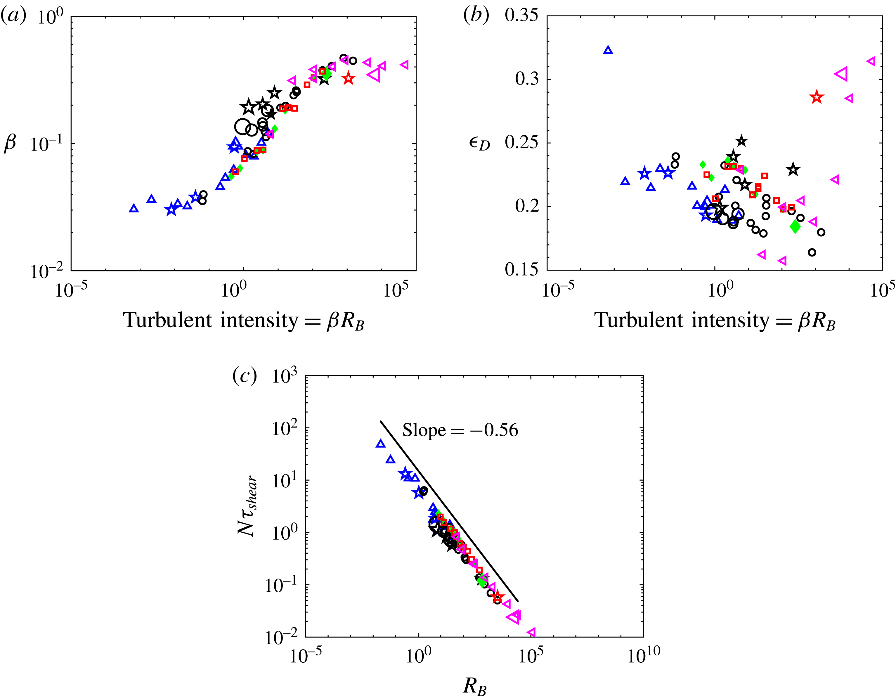
Variation of $\unicode[STIX]{x1D6FD}=\unicode[STIX]{x1D716}_{V}/\unicode[STIX]{x1D716}_{D}$ (a) and $\unicode[STIX]{x1D716}_{D}=u_{rms}^{3}/L_{int}$ (b) with turbulent intensity ${\mathcal{R}}_{I}=\unicode[STIX]{x1D716}_{V}/[\unicode[STIX]{x1D708}N^{2}]=\unicode[STIX]{x1D6FD}{\mathcal{R}}_{B}$ . (c) Shows $Ri^{1/2}\equiv N\unicode[STIX]{x1D70F}_{shear}$ as a function of the buoyancy Reynolds number ${\mathcal{R}}_{B}=ReFr^{2}$ , with $\unicode[STIX]{x1D70F}_{shear}=\langle \unicode[STIX]{x2202}_{z}u_{\bot }\rangle$ . All plots have binning in Rossby number, and symbols are as described in the caption of figure 1. The scaling $N\unicode[STIX]{x1D70F}_{shear}\approx {\mathcal{R}}_{B}^{-0.56}$ extends through regimes I and II with lower ${\mathcal{R}}_{B}$ and $Fr$ , and possibly regime III.

If we now examine the variations of $\unicode[STIX]{x1D6FD}$ with ${\mathcal{R}}_{I}=\unicode[STIX]{x1D716}_{V}/[\unicode[STIX]{x1D708}N^{2}]$ , we see in figure 2(a) that we again have good scaling throughout, with $\unicode[STIX]{x1D6FD}\sim {\mathcal{R}}_{I}^{1/3}\sim \unicode[STIX]{x1D6FD}^{1/3}{\mathcal{R}}_{B}^{1/3}$ . It is easy to show that this is compatible with (3.3), since $\unicode[STIX]{x1D6FD}\sim {\mathcal{R}}_{B}^{1/2}\sim Fr$ , omitting a dependency in $Re^{1/3}$ , although it appears clearly in figure 2 that, at fixed ${\mathcal{R}}_{I}$ and lower $Re$ , $\unicode[STIX]{x1D6FD}$ is measurably larger since $Fr$ is larger. This indicates that care must be taken when interpreting data as a function of dimensionless parameters. In ${\mathcal{R}}_{B}$ , the transitions between the three regimes occur respectively for ${\approx}2$ and ${\approx}200$ . Such values are relevant for example in the ocean thermocline, where ${\mathcal{R}}_{B}\approx 10{-}100$ (Fleury & Lueck Reference Fleury and Lueck1994), as well as in lakes in which an average for ${\mathcal{R}}_{B}$ is ${\approx}200$ (Bouffard & Boegman Reference Bouffard and Boegman2013).

The dimensional kinetic energy dissipation $\unicode[STIX]{x1D716}_{D}$ (figure 2 b) is constant across parameters, and across initial conditions, except for very small or large $Fr$ values. A slight trend towards smaller values at higher ${\mathcal{R}}_{I}$ , which can be attributed to smaller root mean square (r.m.s.) velocities, is discernible. Finally, we show in figure 2(c) that $Ri^{1/2}\sim {\mathcal{R}}_{B}^{-1/2}$ , a scaling compatible with $Ri\sim Fr^{-2}$ at constant Reynolds number. At low $Fr$ , this relation gives the strength of vertical gradients (slanted because of rotation), and at higher $Fr$ , it indicates a progressive return to isotropy and to only a single time scale determining the dynamics, transfer and dissipation of such turbulent flows. Note that the three results in (3.1–3.3) may not be entirely new but, taken together, they define the key ingredients for establishing the scaling of the mixing efficiency which is discussed in § 4.

4 Mixing and dissipation

4.1 Definitions of mixing efficiency and flux Richardson number

Irreversible mixing is found in the laboratory to be triggered by merging Kelvin–Helmholtz billows (Patterson et al. Reference Patterson, Caulfield, McElwaine and Dalziel2006), which are highly unstable as $Re$ increases. In the absence of rotation, parameter space has been separated into three regions in terms of $Fr$ and $Re$ (Luketina & Imberger Reference Luketina and Imberger1989): for small $Re$ and $Fr$ , waves are dominant and there are no turbulent motions, whereas for high $Fr$ and $Re$ , isotropic turbulence prevails. The intermediate region with roughly $Fr\leqslant 1,~{\mathcal{R}}_{B}\geqslant 10$ is where turbulence is anisotropic and strongly interacting with waves. The data on which these conclusions are based come from the analysis of turbulent plumes active in tidal estuary flows (Stillinger, Helland & van Atta Reference Stillinger, Helland and van Atta1983; Stacey, Monismith & Burau Reference Stacey, Monismith and Burau1999). We find similar transitions with mild rotation, as shown in § 3.3.

In terms of the temporal evolution of vertical kinetic and potential energy density, one is led to compare the buoyancy flux $B_{f}=N\langle w\unicode[STIX]{x1D703}\rangle$ with the dissipation rates, the Coriolis force not affecting the energy balance. Performing space averaging, one can write:

(4.1a,b ) $$\begin{eqnarray}\displaystyle & \displaystyle D_{t}E_{V}=-B_{f}+\unicode[STIX]{x1D716}_{V},\quad D_{t}E_{P}=B_{f}+\unicode[STIX]{x1D716}_{P}. & \displaystyle\end{eqnarray}$$

In order to quantify the relative magnitudes of these terms, several expressions have been introduced in the literature. Concerning the momentum equation, one traditionally defines the flux Richardson number $R_{f}$ and its associated mixing efficiency $\unicode[STIX]{x1D6E4}_{f}$ as:

(4.2a,b ) $$\begin{eqnarray}\displaystyle R_{f}=\frac{B_{f}}{B_{f}+\unicode[STIX]{x1D716}_{V}},\quad \unicode[STIX]{x1D6E4}_{f}=\frac{R_{f}}{1-R_{f}}=\frac{B_{f}}{\unicode[STIX]{x1D716}_{V}}. & & \displaystyle\end{eqnarray}$$

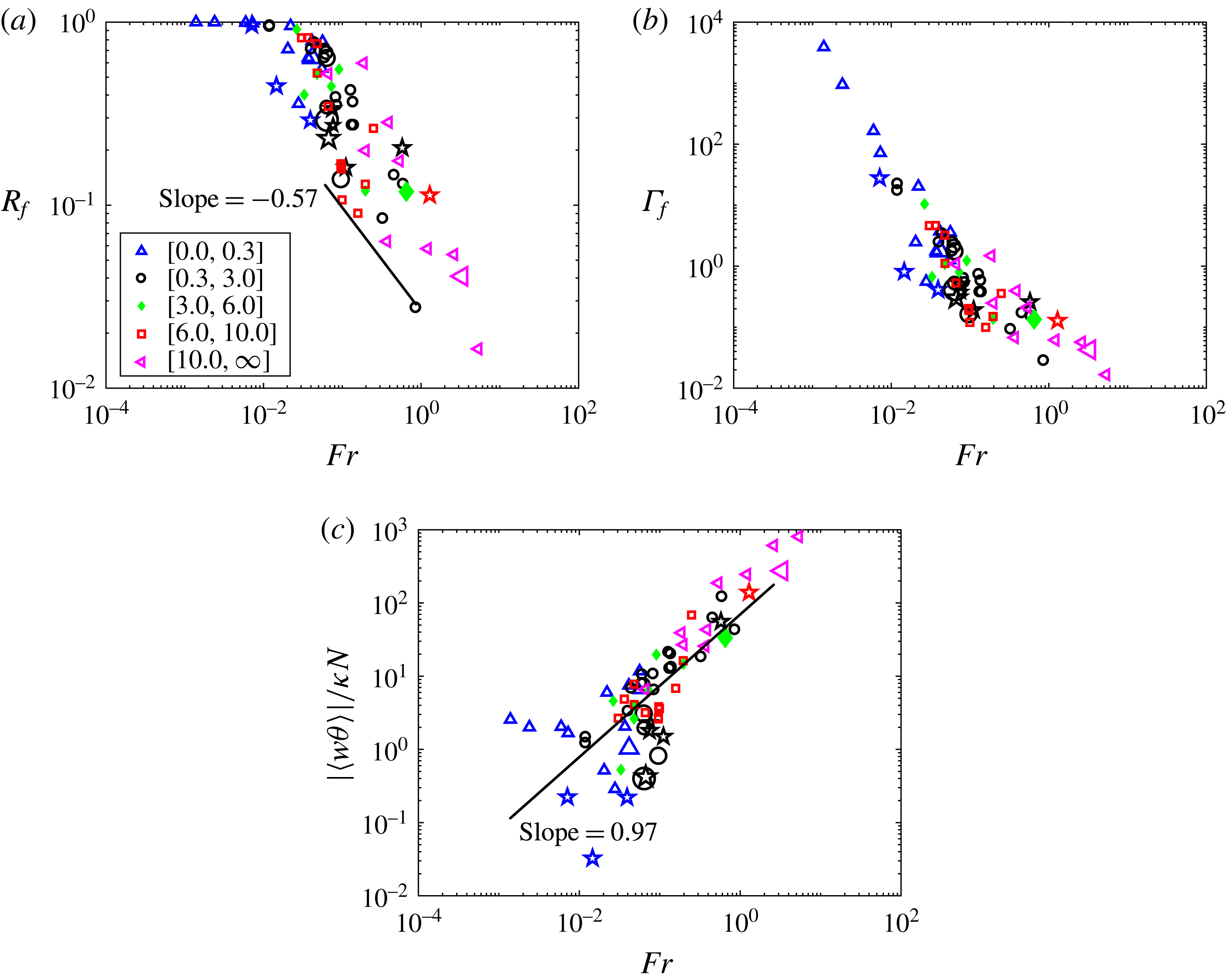
The functional variation of $R_{f}$ with gradient Richardson number is central to numerical studies of geophysical flows. The mixing efficiency $\unicode[STIX]{x1D6E4}_{f}$ is singular for $R_{f}=1$ , i.e. for fully mixed potential and kinetic modes (see Mashayek & Peltier (Reference Mashayek and Peltier2013), Salehipour & Peltier (Reference Salehipour and Peltier2015), Mashayek et al. (Reference Mashayek, Salehipour, Bouffard, Caulfield, Ferrari, Nikurashin, Peltier and Smyth2017) for a discussion on the definitions of mixing efficiency). This corresponds to negligible kinetic energy dissipation, i.e. a limit of zero Froude number. As we shall see in figure 3, $\unicode[STIX]{x1D6E4}_{f}$ does reach high values at low $Fr$ , in excess of $10^{3}$ . Many recent works indicate variations with parameters as $Re$ grows.

Figure 3.

Variation with Froude number of the flux Richardson number $R_{f}$ and of the mixing efficiency $\unicode[STIX]{x1D6E4}_{f}$ (a,b), both defined in (4.2), as well as of the effective diffusivity $\unicode[STIX]{x1D705}_{\unicode[STIX]{x1D70C}}/\unicode[STIX]{x1D705}$ (c), with $\unicode[STIX]{x1D705}_{\unicode[STIX]{x1D70C}}=N^{-1}\langle w\unicode[STIX]{x1D703}\rangle$ . Binning is performed in $Ro$ (see figure 1 for symbols). A transition at $Fr\approx 0.02$ is seen in all three plots. Scalings are given as indications.

4.2 Mixing and effective diffusivity as a function of parameters

We evaluate $\unicode[STIX]{x1D6E4}_{f}$ at peak of dissipation, whereas in Stretch et al. (Reference Stretch, Rottman, Venayagamoorthy, Nomura and Rehmann2010), it is computed as the ratio of two time integrals after more than $90\,\%$ of the energy has dissipated. Since energy decay in turbulence is self-similar, these two methods should lead to comparable scalings. We show in figure 3(a,b) $R_{f}$ and $\unicode[STIX]{x1D6E4}_{f}$ as a function of Froude number. At low $Fr$ , $\unicode[STIX]{x1D716}_{V}$ is negligible compared to $B_{f}$ , and $R_{f}\approx 1$ . A sharp transition occurs for $Fr\approx 0.02$ , with $R_{f}$ decreasing continuously thereafter, with no visible saturation. The decline in $R_{f}$ begins in the intermediate range in which waves and vortices interact strongly. Similarly, $\unicode[STIX]{x1D6E4}_{f}$ shows a transition for $Fr\approx 0.02$ , with a change in slope from $\unicode[STIX]{x1D6E4}_{f}\approx Fr^{-2}$ to ${\approx}Fr^{-1}$ , as $Fr$ grows (approximate scalings), and with a variation of several orders of magnitude. At higher $Fr$ (regimes II and III), a power-law scaling seems likely, as for $R_{f}$ . The variation of $R_{f}$ with Richardson number mirrors its variation in terms of $Fr$ (not shown). Another example of strong variation of $\unicode[STIX]{x1D6E4}_{f}$ is found in Bluteau, Jones & Ivey (Reference Bluteau, Jones and Ivey2013) where $\unicode[STIX]{x1D6E4}_{f}=0.2$ is only valid in the range $7<{\mathcal{R}}_{B}<100$ , whereas we find it for $100\lesssim {\mathcal{R}}_{B}\lesssim 1000$ .

The overall variation of $\unicode[STIX]{x1D6E4}_{f}$ with $Fr$ and ${\mathcal{R}}_{B}$ is similar to that found in the absence of rotation but with shear (Mater & Venayagamoorthy Reference Mater and Venayagamoorthy2014). These authors further note that the centroid of such a curve depends on what flows are studied, as for example in the data of Lozovatsky & Fernando (Reference Lozovatsky and Fernando2013) where the centroid is shifted to higher ${\mathcal{R}}_{B}$ . This presents a challenge, since parameterization schemes are mostly based on DNS, which may still be at too low a value of ${\mathcal{R}}_{B}$ , and since using ${\mathcal{R}}_{B}$ implies studying variations in terms of both stratification (through $Fr$ ) and of turbulence (through $Re$ ). The variations with Reynolds and buoyancy Reynolds numbers are discussed further in § 7.

Figure 4.

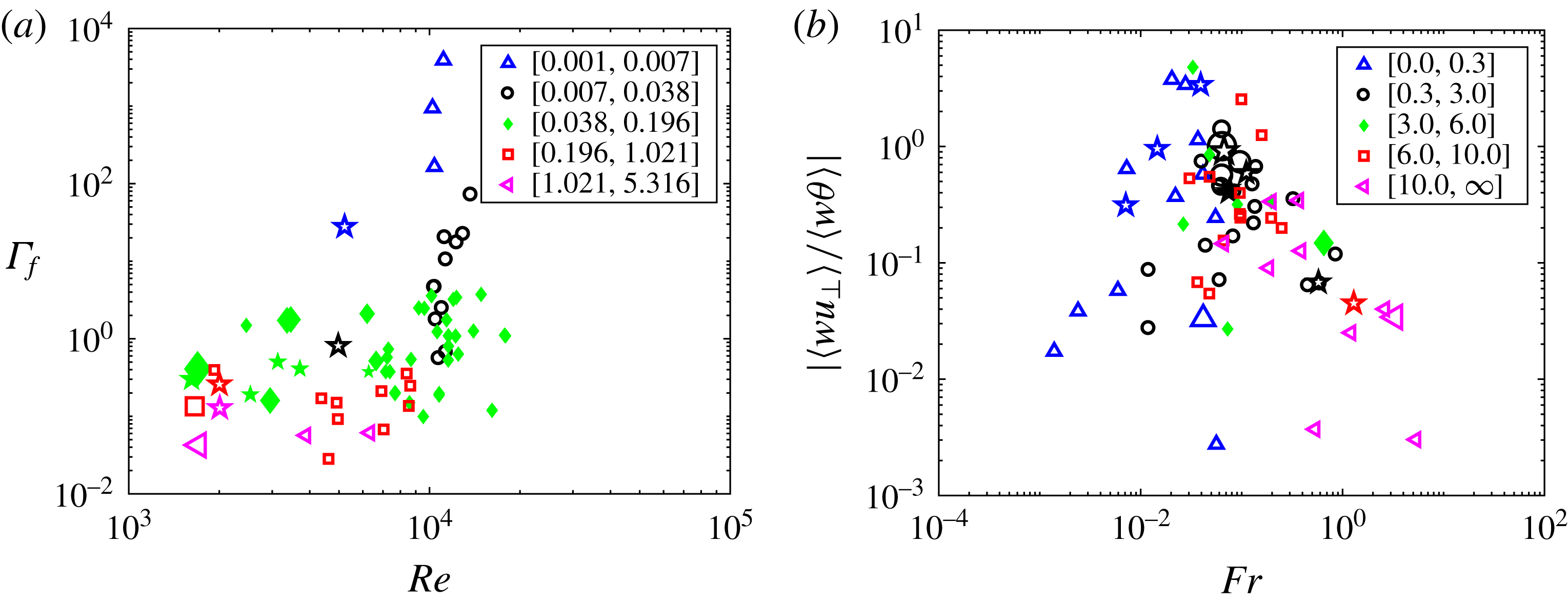
(a) Variation of mixing efficiency $\unicode[STIX]{x1D6E4}_{f}$ with Reynolds number, with binning in Froude number (see inset). (b) Variation with $Fr$ of the ratio of the vertical flux of horizontal velocity to the vertical flux of buoyancy, with binning in Rossby number. The size of symbols for both plots is described in the caption of figure 1.

In figure 3(c) we plot the effective diffusivity $\unicode[STIX]{x1D705}_{\unicode[STIX]{x1D70C}}$ , relative to the molecular diffusivity $\unicode[STIX]{x1D705}$ . It is proportional to the buoyancy flux $B_{f}$ . Taking the notation in Ivey et al. (Reference Ivey, Winters and Koseff2008):

(4.3a,b ) $$\begin{eqnarray}\displaystyle \unicode[STIX]{x1D705}_{\unicode[STIX]{x1D70C}}=B_{f}/N^{2},\quad \unicode[STIX]{x1D705}_{\unicode[STIX]{x1D70C}}/\unicode[STIX]{x1D705}=\langle w\unicode[STIX]{x1D703}\rangle /[N\unicode[STIX]{x1D705}]; & & \displaystyle\end{eqnarray}$$

$\unicode[STIX]{x1D705}_{\unicode[STIX]{x1D70C}}$ is comparable to $\unicode[STIX]{x1D705}$ at low $Fr$ , and its increase with $Fr$ is close to a linear variation, a least-square fit giving $\unicode[STIX]{x1D705}_{\unicode[STIX]{x1D70C}}/\unicode[STIX]{x1D705}\approx Fr^{0.97}$ . Finally, a saturation begins to occur at high $Fr$ . This behaviour can be interpreted as being due to an increase in buoyancy flux because of more vigorous stirring when ${\mathcal{R}}_{B}$ increases, at relatively constant $Re$ . When comparing the high- $Fr$ values of $\unicode[STIX]{x1D705}_{\unicode[STIX]{x1D70C}}/\unicode[STIX]{x1D705}$ to the model proposed in Barry et al. (Reference Barry, Ivey, Winters and Imberger2001), a rough agreement is obtained. Similarly, when examining a compilation of observational data for both salinity and temperature in the ocean together with numerical data for purely stratified flows, it is found in Bouffard & Boegman (Reference Bouffard and Boegman2013) that a transition occurs in $\unicode[STIX]{x1D705}_{\unicode[STIX]{x1D70C}}$ , at ${\mathcal{R}}_{B}\approx 100$ , between a ${\mathcal{R}}_{B}^{3/2}$ and a ${\mathcal{R}}_{B}^{1/2}$ scaling (see also Shih et al. (Reference Shih, Koseff, Ivey and Ferziger2005) for the latter). This enhancement of dissipation and of transport coefficients, such as anomalous diffusivity, is expected in turbulent flows as shown in numerous studies of FDT (Ishihara, Gotoh & Kaneda Reference Ishihara, Gotoh and Kaneda2009), as well as in the strongly stratified case (Ivey et al. Reference Ivey, Winters and Koseff2008). In this latter instance, it is probably due to strong intermittency, a signature of strongly stably stratified flows (Rorai et al. Reference Rorai, Mininni and Pouquet2014), such as in the planetary boundary layer (Finnigan Reference Finnigan1999), or in the ocean (D’Asaro et al. Reference D’Asaro, Lee, Rainville, Harcourt and Thomas2011).

We show in figure 4(a) the mixing efficiency $\unicode[STIX]{x1D6E4}_{f}$ as a function of Reynolds number. Around $Re\approx 10^{4}$ , which covers many of the runs of table 1, $\unicode[STIX]{x1D6E4}_{f}$ takes on a variety of values corresponding to how strongly the flow is stratified, with variations in excess of 1000. However, at lower $Re$ (for most of the runs of table 2), $\unicode[STIX]{x1D6E4}_{f}$ remains at lower values, the peak in $\unicode[STIX]{x1D6E4}_{f}$ being linked to the development of small-scale instabilities as $Re$ and ${\mathcal{R}}_{B}$ grow. Finally, another measure of the small-scale mixing efficiency of a flow is the ratio of the vertical fluxes of horizontal velocity to that of temperature fluctuations, as analysed in Zilitinkevich et al. (Reference Zilitinkevich, Elperin, Kleeorin, Rogachevskii and Esau2013). It is shown in figure 4(b) as a function of $Fr$ ; no clear scaling emerges although one could advocate a $Fr^{-1}$ decrease for regimes II and III. Also, this ratio appears to be higher in the intermediate regime, on average.

Figure 5.

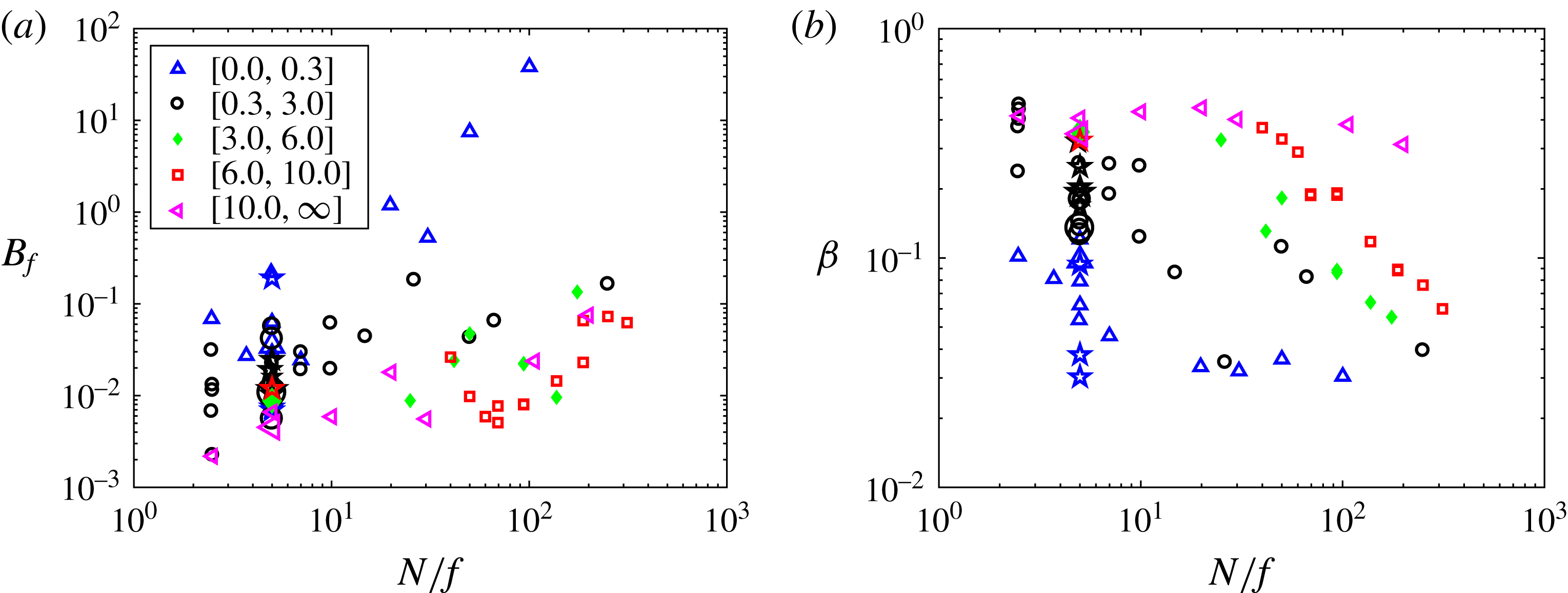
Variation with $N/f=Ro/Fr$ of the buoyancy flux $B_{f}=\langle Nw\unicode[STIX]{x1D703}\rangle$ (a), and of the dissipation efficiency $\unicode[STIX]{x1D6FD}=\unicode[STIX]{x1D716}_{V}/\unicode[STIX]{x1D716}_{D}$ (b), with binning in $Ro$ (see inset); symbols are as in figure 1. For a given $N/f$ , both can take a large range of values.

5 The combined roles of rotation and stratification

The addition of rotation leads to the propagation of inertia–gravity waves whose dispersion relation depends on $N/f$ . Thus, the atmosphere, with $N/f\sim 100$ , and the ocean where $N/f\lesssim 10$ may differ in their statistical properties. For all runs of this paper, $N/f\geqslant 2.5$ , so that stratification dominates. It is thus not surprising that the classical picture of mixing in stratified flows has not been changed in a significant way when weak rotation is included but in the absence of scale separation and of forcing. We do see an effect of rotation on the magnitude of the potential energy (see e.g. figure 1 a), strong rotation altering the large scales where the energy is contained. It was shown in Marino et al. (Reference Marino, Pouquet and Rosenberg2015a ) that rotation and stratification play complementary roles in the relative strength of the direct and inverse constant-flux energy cascades in the forced case: the small-scale cascade is weaker the smaller the Froude number, and conversely the large-scale cascade is stronger the smaller $Ro$ is, in both cases affecting the effective dissipation of energy in the small scales and thus, presumably, the mixing properties of such flows. For the flows of table 1, all micro Rossby numbers, $R_{\unicode[STIX]{x1D714}}=\unicode[STIX]{x1D714}_{rms}/f$ , are larger than $3.1$ , with $Ro\geqslant 0.11$ . Thus, the small-scale vorticity created by the nonlinear dynamics of the flow, including in the presence of strong waves, is dominant at small scale, compared to the imposed rotation; note that such values for $R_{\unicode[STIX]{x1D714}}$ are plausible for geophysical flows.

Figure 5(a,b) gives the variations with $N/f$ of the buoyancy flux $B_{f}$ and of the dissipation efficiency $\unicode[STIX]{x1D6FD}$ . At a given $N/f$ , there is less buoyancy flux the higher the Rossby number, and for a given bin in $Ro$ , $B_{f}$ is larger the higher $N/f$ : as the Froude number increases, the buoyancy flux decreases. The efficiency of dissipation is higher the higher the Rossby number (figure 5 b), again at fixed $N/f$ . Perhaps the scaling of $\unicode[STIX]{x1D6FD}$ with $Fr$ is somewhat modified by rotation, leading to the slightly sub-linear law observed in figure 1(c); there may be less direct energy transfer for strong rotation, as is observed in the forced case (Marino et al. Reference Marino, Pouquet and Rosenberg2015a ), and thus it takes a higher Froude number to reach a given level of dissipation. A clear effect of the Rossby number on dissipation in RST was also shown in the forced case in Pouquet et al. (Reference Pouquet, Marino, Mininni and Rosenberg2017).

Thus, the absence in the overall statistical properties of clear scaling in $Ro$ simply shows that the energy transfer to the small scales is dominated by a combination of stratification and turbulence. However, the primary purpose of this study is not to examine the role of rotation directly. Such a study would be helped by analysing flows with $N/f<1$ , a parameter range which is relevant neither to the atmosphere nor to the ocean. For $N/f>1$ , the most important role of rotation in such flows is the triggering of an inverse cascade of energy to the large scales, attenuating the energy transfer to the small scales (Pouquet & Marino Reference Pouquet and Marino2013; Marino et al. Reference Marino, Pouquet and Rosenberg2015a ; Pouquet et al. Reference Pouquet, Marino, Mininni and Rosenberg2017). In the absence of forcing and of scale separation, such an inverse cascade cannot develop in general.

6 The Ellison scale and a generalized mixing efficiency

Figure 6.

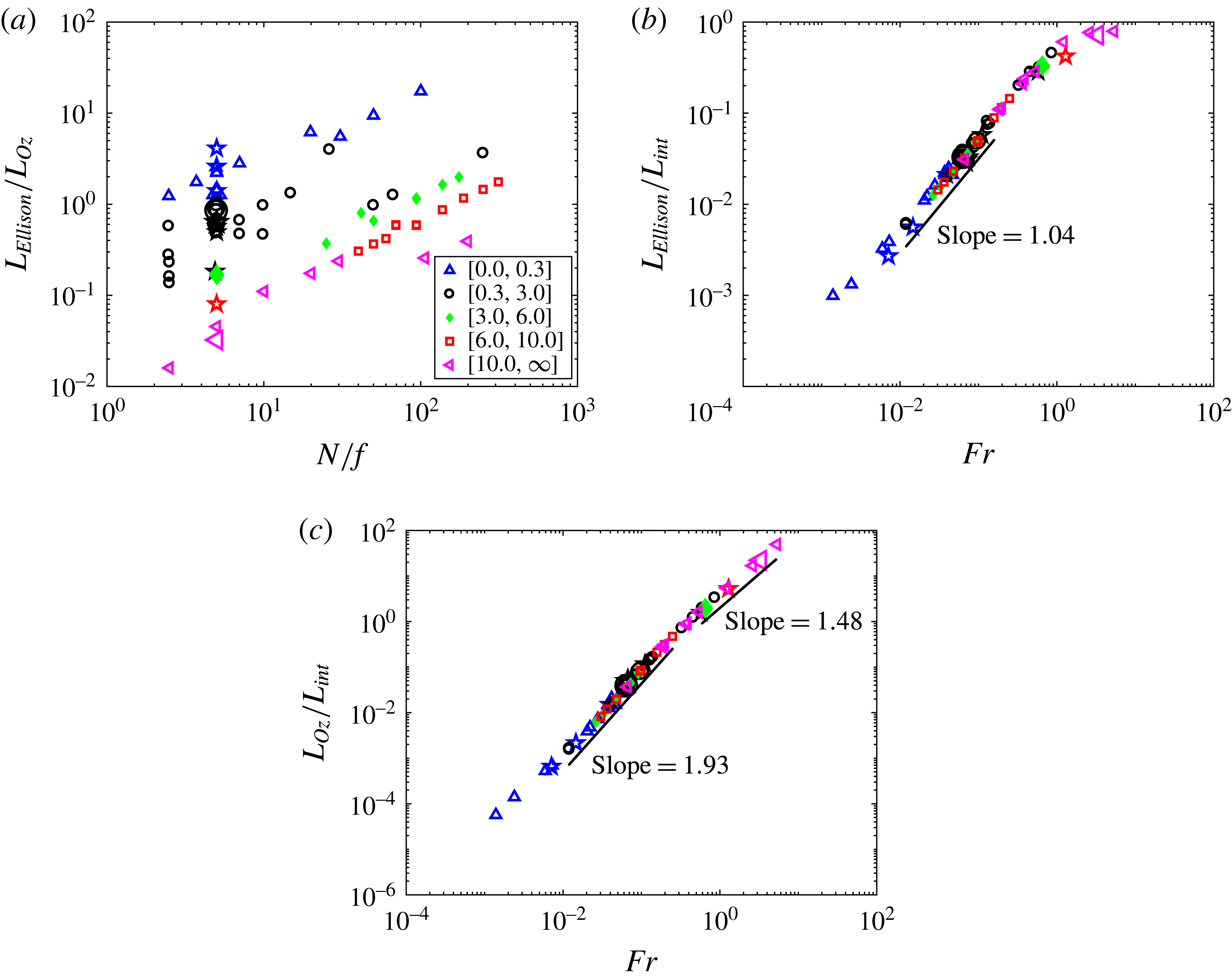
Ellison scale $L_{Ell}=\unicode[STIX]{x1D703}_{rms}/N$ relative to the Ozmidov scale $\ell _{Oz}$ (a) or the integral scale $L_{int}$ (b), as a function of $N/f$ (a), and of $Fr$ (b). (c) $\ell _{Oz}/L_{int}$ as a function of $Fr$ . All plots have binning in $Ro$ (and see caption of figure 1). Note the small dispersion in the scaling of length scales versus Froude number (approximate scalings are given).

Similarly to characteristic time scales, one can also examine characteristic length scales. A comparison of the Thorpe and Ellison scales in stratified turbulence was performed in Mater et al. (Reference Mater, Schaad and Venayagamoorthy2013) (see also Dillon (Reference Dillon1982)). The Thorpe scale $L_{T}$ corresponds to the vertical distance a parcel of fluid must be moved to produce a stable density profile, suppressing inversions, and as such gives an idea of the size of local mixing structures in the fluid; it was computed as a function of ${\mathcal{R}}_{B}$ for the purely stratified case in Métais & Herring (Reference Métais and Herring1989). In Mater et al. (Reference Mater, Schaad and Venayagamoorthy2013), $L_{T}$ is found to be strongly linearly correlated with the Ellison scale $L_{Ell}$ . Furthermore, the Thorpe length normalized by the Ozmidov scale is found to vary as $Fr^{-3/2}$ for $Fr>1$ and as $Fr^{-1/2}$ for $Fr<1$ , the latter with an excellent scaling for $0.05\leqslant Fr\leqslant 0.3$ . Thus, $L_{T}\sim L_{B}$ for $Fr<1$ , whereas $L_{T}\sim L_{int}$ for $Fr>1$ . In the latter case, stratification is weak and structures in density follow the integral length scale, whereas in the former case of strong stratification, density changes occur over the vertical layer width, i.e. the buoyancy scale. Note that this also implies that, at small Froude number, $L_{T}/L_{int}\sim Fr$ and that $E_{P}\sim E_{V}$ (Mater et al. Reference Mater, Schaad and Venayagamoorthy2013).

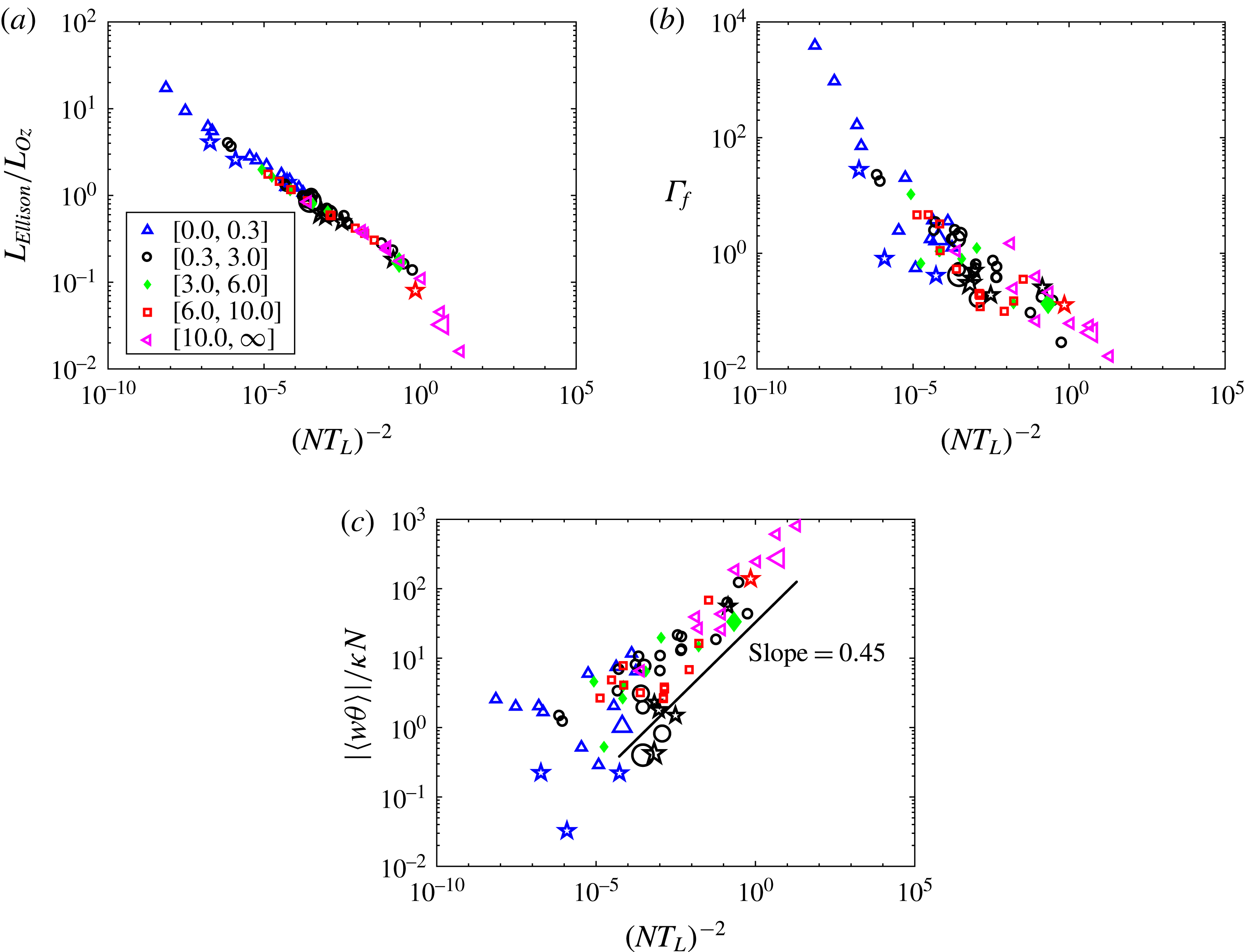
Figure 6 shows the variations of $L_{Ell}$ normalized by the Ozmidov scale (a) and integral scale (b), as a function of $N/f$ (a), and of $Fr$ (b), with binning in Rossby number. We conclude that the Ellison scale is larger, the larger $Fr$ is, as expected. As a function of Froude number, $L_{Ell}/\ell _{Oz}$ decreases, in a linear fashion for the intermediate regime, and with little dispersion among the runs (not shown). One could argue that with $\ell _{Oz}=[\unicode[STIX]{x1D716}_{V}/N^{3}]^{1/2}$ , for small Froude number, $\ell _{Oz}/L_{int}\sim Fr^{2}$ in the intermediate regime in which $\unicode[STIX]{x1D6FD}\sim Fr$ , whereas for high $Fr$ , $\ell _{Oz}/L_{int}\sim Fr^{3/2}$ , in rough agreement with scaling laws, as indicated in figure 6(c) giving $\ell _{Oz}/L_{int}=f(Fr)$ with least-square fits of respectively $1.93$ and $1.48$ , the transitions taking place for $Fr\approx 0.01$ and $Fr\approx 0.2$ , in agreement with the transitions for $\unicode[STIX]{x1D6FD}$ (see figure 1 c).

On the other hand, the linear variation $L_{Ell}/L_{int}\sim Fr$ in figure 6(b), with a least-square fit giving ${\sim}Fr^{1.04}$ , is a direct consequence of the scaling law $\unicode[STIX]{x1D703}_{rms}\sim u_{rms}$ . The only transition in this power-law behaviour takes place for $Fr=O(1)$ , in which case $L_{Ell}\lesssim L_{int}$ , with $L_{Ell}$ remaining smaller than $L_{int}$ because of the $1/k$ factor in the definition of $L_{int}$ . There is also an indication of a slight saturation at low $Fr$ .

Another measure of the relative importance of terms in the Boussinesq equations is defined through the ratio of the two dissipative terms for momentum and temperature, which can differ even at unit Prandtl number. We use the following definitions (see also Osborn (Reference Osborn1980), Venayagamoorthy & Koseff (Reference Venayagamoorthy and Koseff2016)):

(6.1a,b ) $$\begin{eqnarray}\displaystyle & \displaystyle R_{f}^{\ast }=\frac{\unicode[STIX]{x1D716}_{P}}{\unicode[STIX]{x1D716}_{T}},\quad \unicode[STIX]{x1D6E4}_{f}^{\ast }=\frac{R_{f}^{\ast }}{1-R_{f}^{\ast }}=\frac{\unicode[STIX]{x1D716}_{P}}{\unicode[STIX]{x1D716}_{V}}, & \displaystyle\end{eqnarray}$$

with $\unicode[STIX]{x1D716}_{T}=\unicode[STIX]{x1D716}_{V}+\unicode[STIX]{x1D716}_{P}$ already defined in (2.5). $\unicode[STIX]{x1D6E4}_{f}^{\ast }$ , called the irreversible mixing efficiency in Mater & Venayagamoorthy (Reference Mater and Venayagamoorthy2014), relates to the partition of energy dissipation between the kinetic and potential modes, i.e. to the importance of the waves versus nonlinear eddies at small scales. 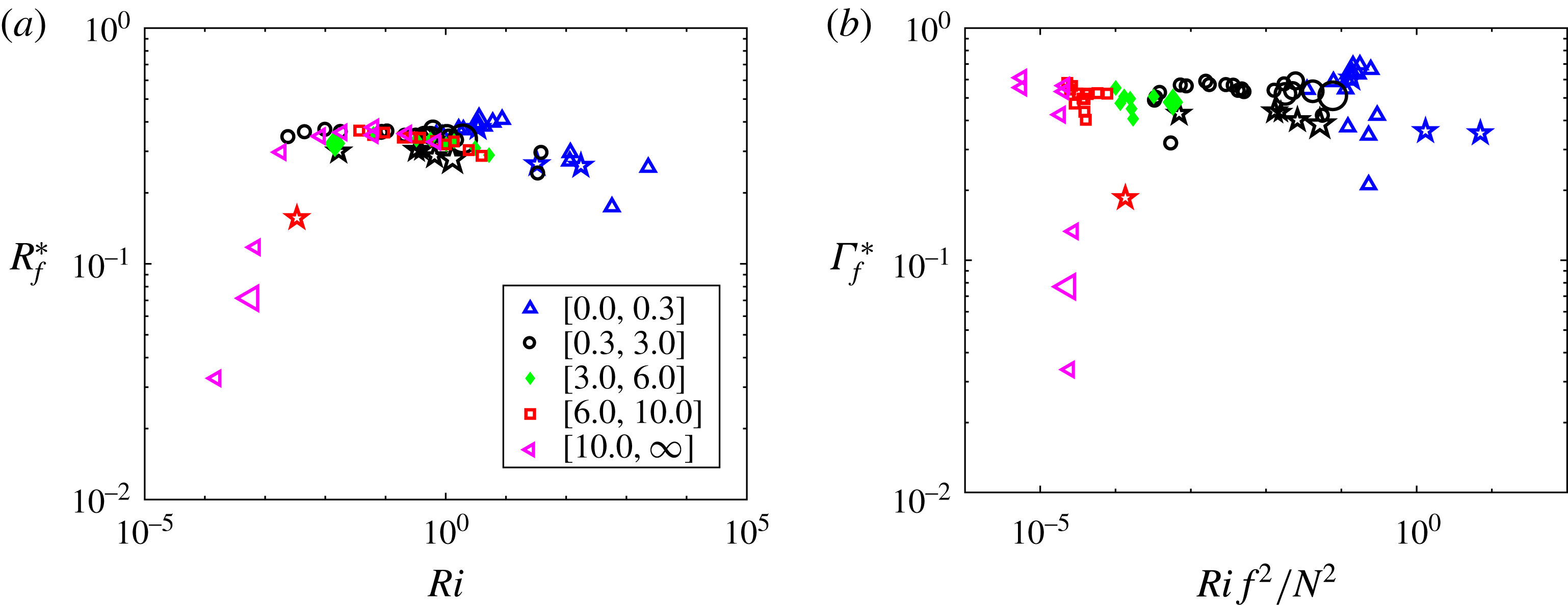$R_{f}^{\ast }$ is shown in figure 7(a) as a function of Richardson number $Ri$ . In the first regime of strong waves ( $Ri>1$ ), it is small since the influence of initial conditions prevails, and similarly for the low $Ri$ regime in which the potential–kinetic exchanges are inefficient, leading to an abrupt decrease in $R_{f}^{\ast }$ . For intermediate values of $Ri$ , almost from $10^{-3}$ to roughly $10$ , $R_{f}^{\ast }$ stays rather constant in a range between $0.3$ and $0.4$ . Note also that these data are consistent with the variations of $\unicode[STIX]{x1D716}_{V}$ and $\unicode[STIX]{x1D716}_{P}$ with $Fr$ studied in Sozza et al. (Reference Sozza, Boffetta, Muratore-Ginanneschi and Musacchio2015) in a thin layer box.

Figure 7.

Potential energy dissipation normalized by total dissipation, $R_{f}^{\ast }=\unicode[STIX]{x1D716}_{P}/\unicode[STIX]{x1D716}_{T}$ , versus Richardson number $Ri$ (a), and $\unicode[STIX]{x1D6E4}_{f}^{\ast }=\unicode[STIX]{x1D716}_{P}/\unicode[STIX]{x1D716}_{V}$ versus $Rif^{2}/N^{2}=[\unicode[STIX]{x1D70F}_{shear}f]^{2}$ (b). Binning is performed in $Ro$ (see inset, and caption of figure 1).

We finally examine in figure 7(b) the variations of $\unicode[STIX]{x1D6E4}_{f}^{\ast }$ with $Rif^{2}/N^{2}=[\unicode[STIX]{x1D70F}_{shear}f]^{2}$ , thus combining the effects of stratification and rotation. A rather small variation of $\unicode[STIX]{x1D6E4}_{\ast }\approx 0.5$ is obtained, with the low points corresponding to small $f$ . There is a slow decline for small $Ro$ and large $Ri$ which may be related to sensitivity to initial conditions at low $Fr$ : in regime I, $\unicode[STIX]{x1D716}_{V}\approx \unicode[STIX]{x1D716}_{P}$ is compatible with $E_{P}\approx E_{V}$ since, when the waves are strong to moderate, there is little nonlinear transfer and the dissipation is mostly contained in the large scales. Also, the highest value of $\unicode[STIX]{x1D6E4}_{f}^{\ast }\approx 0.7$ for $Fr\approx 0.01$ , corresponds obviously to flows with comparable kinetic and potential energy dissipation. This is likely associated in that regime with strong waves and intermittent bursts which are due to wave breaking which temporarily relax the flow to a quasi-equipartition of kinetic and potential energies across a wide range of scales, the more so the smaller the scale, as observed for example in Rosenberg et al. (Reference Rosenberg, Pouquet, Marino and Mininni2015). Our results corroborate those of Venayagamoorthy & Koseff (Reference Venayagamoorthy and Koseff2016): different measures of mixing, such as $\unicode[STIX]{x1D6E4}_{f}$ or $\unicode[STIX]{x1D6E4}_{f}^{\ast }$ , give rather equivalent information, although it is not clear if this result will persist in the presence of forcing, at much higher buoyancy Reynolds numbers.

7 Role of Reynolds number

The variation of the intensity of the turbulence in rotating stratified flows can be measured by the Reynolds number, as well as by the buoyancy Reynolds number. Having high enough $Re$ and ${\mathcal{R}}_{B}$ is known to be important for turbulent flows, to allow for coherent structures to develop including in the presence of strong stratification (see e.g. Laval, McWilliams & Dubrulle (Reference Laval, McWilliams and Dubrulle2003)). However, from a numerical point of view, having high $Re,{\mathcal{R}}_{B}$ for low $Fr$ is quite challenging and remains a goal for the near future. 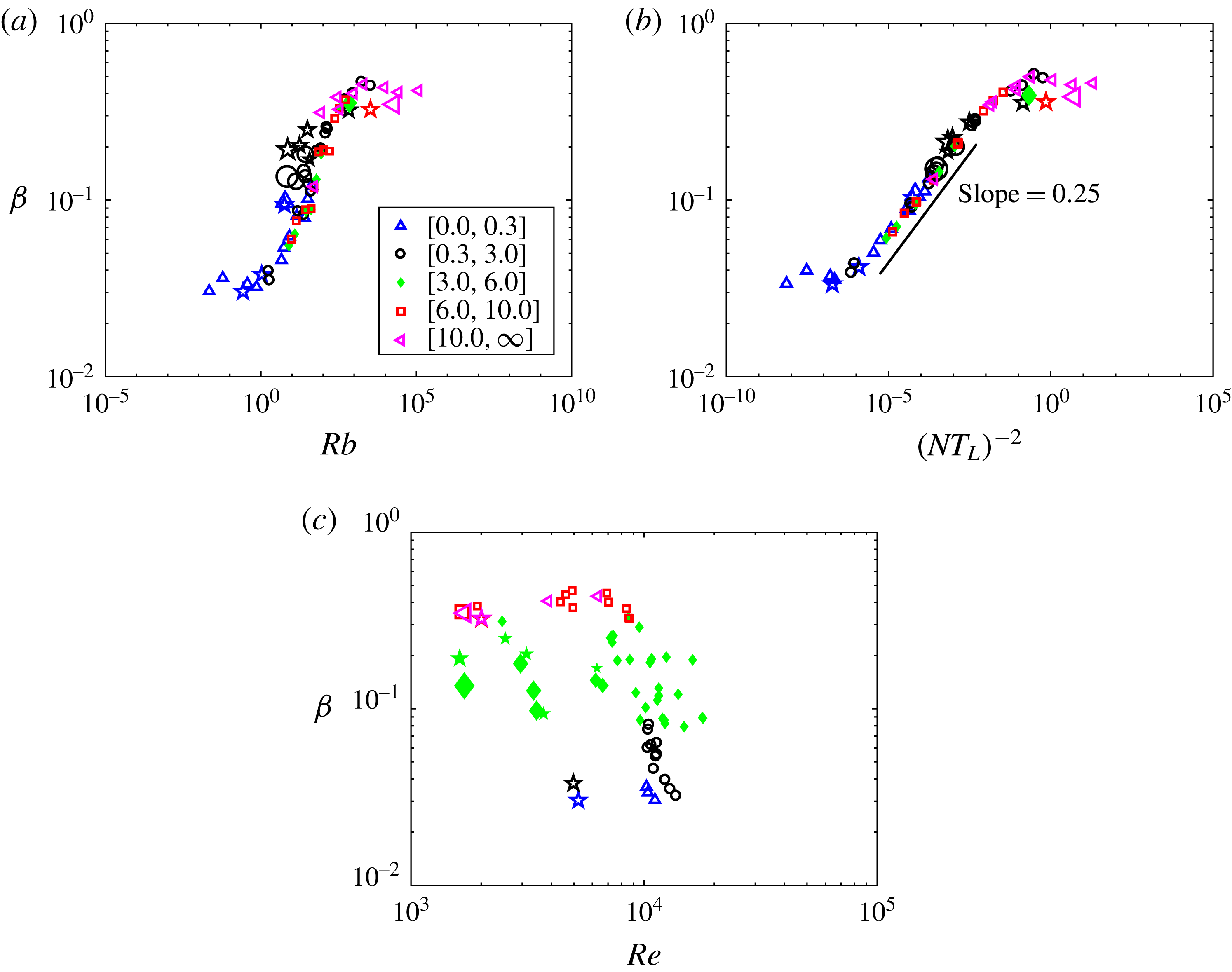When taking the data for the runs of tables 1 and 2 for a possible scaling of the dissipation efficiency $\unicode[STIX]{x1D6FD}$ with ${\mathcal{R}}_{B}$ , we observe some scatter (see figure 8 a). Specifically, we see that in the intermediate regime ( ${\mathcal{R}}_{B}$ between 10 and a few $100$ ), at fixed ${\mathcal{R}}_{B}$ , there is a measurable variation in $\unicode[STIX]{x1D6FD}$ , by contrast to regime I, and to a lesser extent regime III. This scatter in regime II is larger than when examining variations with the Froude number itself, irrespective of the rotation (see figure 1 c). In figure 8 b, we see that overall, there is markedly less scatter when plotting $\unicode[STIX]{x1D6FD}$ as a function of the parameter $[NT_{L}]^{-2}$ as discussed in Mater & Venayagamoorthy (Reference Mater and Venayagamoorthy2014) (see § A.1), with $T_{L}\equiv E_{V}/\unicode[STIX]{x1D716}_{V}$ the effective kinetic energy transfer time. Expressing $\unicode[STIX]{x1D716}_{V}=\unicode[STIX]{x1D6FD}\unicode[STIX]{x1D716}_{D}$ , we see that $NT_{L}=[\unicode[STIX]{x1D6FD}Fr]^{-1}$ ; thus, the choice of the abscissa in figure 8(b) is to be able to make a direct comparison with ${\mathcal{R}}_{B}$ which scales as $Fr^{2}$ at fixed $Re$ . We also note that the regime transitions in terms of Richardson number occur for $Ri\approx 0.1$ and $Ri\approx 10$ (not shown).

The difference in data point scatter between figure 8(a,b) can be attributed to the variations with Reynolds number, as displayed in figure 8(c). It shows clearly that the Reynolds number alone does not allow for predicting the effectiveness of dissipation, and consequently that of mixing efficiency, with a wide scattering of data points for $\unicode[STIX]{x1D6FD}$ , irrespective of the initial conditions tested in this paper. However, we see that at a given $Re$ , QG initial conditions lead to a substantially lower dissipation efficiency. We further note that Reynolds numbers are still quite low for these runs, when comparing with geophysical flows. Similar conclusions can be drawn for the variation with $Re$ of the ratio of the Ellison scale normalized by the integral scale (not shown). Finally, in order to connect with laboratory experiments in particular, it might be useful to study more in depth regime I at low ${\mathcal{R}}_{B}$ , so that one can investigate the possibility of a dependence on $Re$ of the dissipation efficiency $\unicode[STIX]{x1D6FD}$ because of viscous coupling between layers (Riley & deBruynKops Reference Riley and deBruynKops2003; Brethouwer et al. Reference Brethouwer, Billant, Lindborg and Chomaz2007).

Figure 8.

Dissipation efficiency $\unicode[STIX]{x1D6FD}=\unicode[STIX]{x1D716}_{V}/\unicode[STIX]{x1D716}_{D}$ as a function of (a) ${\mathcal{R}}_{B}$ ; (b) $[NT_{L}]^{-2}$ ; (c) $Re$ (see § A.1 for a discussion of $NT_{L}=NE_{V}/\unicode[STIX]{x1D716}_{V}$ ). Note the scaling $\unicode[STIX]{x1D6FD}\sim [NT_{L}]^{-1/2}$ in (b).

8 Discussion, conclusion and perspectives

A parametric study of mildly rotating stratified turbulence without forcing leads to a rather systematic quantitative assessment of its mixing and dissipative properties which depend on the Froude number provided the Reynolds number is high enough. Three different regimes are observed, in agreement with previous studies of purely stratified flows. These regimes are also identifiable in terms of the interaction parameter ${\mathcal{R}}_{I}$ . The three basic laws illustrated in figure 1 are compatible with an intermediate regime characterized by the dynamics of waves and eddies interacting nonlinearly weakly, even though the full weak turbulence formalism leading to a set of closed integro–differential equations in terms of energy spectra cannot work for stratified flows when the Froude number in the vertical is of order unity (Billant & Chomaz Reference Billant and Chomaz2001). It is thus somewhat remarkable that the simple phenomenology embodied in the parameter $\unicode[STIX]{x1D6FD}\sim Fr$ , i.e. the efficiency of the turbulent dissipation, based on a ratio of characteristic time scales (see (A 4)), may still apply on average for such flows.

Together with $\unicode[STIX]{x1D703}_{rms}\sim u_{rms}$ and a scaling for $w/u_{\bot }$ going as a quasi-constant at intermediate $Fr$ , these laws imply that the mixing efficiency $\unicode[STIX]{x1D6E4}_{f}\sim Fr^{-2}$ as soon as $Fr>0.01$ , and $\unicode[STIX]{x1D6E4}_{f}\sim Fr^{-1}\sim {\mathcal{R}}_{B}^{-1/2}$ for $Fr\lesssim O(1)$ . We emphasize that the actual values of the control parameter for the change of regimes may depend on the geometry and topology of such flows. In the intermediate regime, $\unicode[STIX]{x1D6FD}\sim Fr$ , showing the connection between buoyancy flux and nonlinear transfer leading to dissipation, with $\unicode[STIX]{x1D6E4}_{f}\unicode[STIX]{x1D6FD}^{2}\sim 1$ . Note that, with ${\mathcal{R}}_{I}\sim Fr{\mathcal{R}}_{B}$ , this scaling law in the intermediate regime differs when expressed using ${\mathcal{R}}_{I}$ . Finally the mixing efficiency measured in terms of the ratio of potential to kinetic energy dissipation, is shown to be rather constant. The scaling $\unicode[STIX]{x1D6E4}_{f}\sim Fr^{-1}\sim {\mathcal{R}}_{B}^{-1/2}$ , in regime III at high $Fr$ and ${\mathcal{R}}_{B}$ , simply stems from the decoupling of the velocity and temperature, together with $\unicode[STIX]{x1D6FD}\approx 1$ , leading to $B_{f}\sim N$ .

Note also that $\unicode[STIX]{x1D6E4}_{f}$ and $R_{f}$ seem to be more sensitive to parameters with a clear indication of the three physical regimes in terms of $Fr$ , ${\mathcal{R}}_{B}$ or ${\mathcal{R}}_{I}$ , than either $\langle wu_{\bot }\rangle /\langle w\unicode[STIX]{x1D703}\rangle$ or $E_{P}/E_{V}$ . Furthermore, if $w^{2}/u_{\bot }^{2}\sim Fr$ as advocated in Maffioli & Davidson (Reference Maffioli and Davidson2016), then the phenomenological arguments developed in our paper lead straightforwardly to $\unicode[STIX]{x1D6E4}_{f}\sim {\mathcal{R}}_{B}^{-3/4}$ , which cannot be entirely ruled out given the scatter in data points for $\unicode[STIX]{x1D6E4}_{f}$ , although it is not compatible with the data of figure 1(b) with $w_{rms}/u_{rms}\sim 1$ . We verified that taking as initial conditions geostrophically balanced flows did not alter our conclusions; similarly, having non-zero potential energy, but still unbalanced and with $w\not =0$ ICs, we obtained the same fundamental scalings.

Local variations in Richardson number may trigger local density micro-structures, as observed in the ocean (Phillips Reference Phillips1972; Peltier & Caulfield Reference Peltier and Caulfield2003). If the agreement of our results, without shear but with rotation, with previous results mainly for sheared purely stratified flows is striking, it remains to be seen whether it will persist in the presence of forcing, i.e. in the presence of a strong inverse cascade. We note that Waite & Bartello (Reference Waite and Bartello2006) already observed three regimes in the presence of forcing, with a switch for the energy cascade from predominantly inverse to direct.

Within the confines of the present parametric study with a wide range of buoyancy Reynolds numbers, $\unicode[STIX]{x1D6E4}_{f}$ is in fact rather variable, as in the purely stratified case. Rotation is essential for the existence of a dual constant-flux cascade of energy, implying two-dimensional (horizontal) lateral mixing as well as vertical. If such mixing occurs in proportion to the ratio of the inverse to direct cascade, it will scale as $[RoFr]^{-1}$ (Marino et al. Reference Marino, Pouquet and Rosenberg2015a ). In the absence of forcing, with large-scale initial conditions and with rotation weaker than stratification, all effects associated with the presence of rotation are severely quenched. As discussed in Mashayek & Peltier (Reference Mashayek and Peltier2013), shear can induce vortex pairing at moderate Reynolds number, reinforcing the potential for an inverse cascade in the presence of rotation but, on the other hand, as $Re$ increases, three-dimensional instabilities take over and shearing leads to enhanced dissipation.

Another issue, when incorporating rotation or stratification, will be to consider the role of anisotropy on statistics, spectra and structures, the role of non-local interactions among scales, and the role of potential vorticity $P_{V}$ and the magnitude of its nonlinear part; these will be the topic of future work. Several other extensions of the present study are desirable. On the one hand, a larger scanning in terms of Reynolds numbers is needed, but only feasible today at values comparable to or lower than what is presently achieved in this paper, without using modelling such as eddy viscosity or hyper-viscosity, or some other partial truncation of modes such as computing in boxes with small aspect ratio. From the numerical standpoint, the condition $\ell _{Oz}\gg \unicode[STIX]{x1D702},~{\mathcal{R}}_{I}\gg 1$ for strong and stratified turbulence to develop is hard to fulfil even with resolutions allowed by high-performance computing using available present-day technology. For example, in de Bruyn Kops (Reference de Bruyn Kops2015), the highest buoyancy Reynolds number that is reached, on a grid of $8192^{2}\times 4096$ points, is ${\approx}220$ , still quite low compared to atmospheric and oceanic values (see also Iyer et al. (Reference Iyer, Sreenivasan and Yeung2017) for a FDT run on a grid of $8192^{3}$ points with a Taylor Reynolds number of $1300$ ). In the context of the turbulent planetary boundary layer (see e.g. Sukoriansky, Galperin & Staroselsky (Reference Sukoriansky, Galperin and Staroselsky2005)), one can write simplified expressions for vertical mixing, governed by vertical velocity, and horizontal mixing on the basis of a return to isotropy model; this leads to agreement between these models, and laboratory and atmospheric data. One can also model the time evolution of a mixing event by following characteristic length scales (Smyth et al. Reference Smyth, Moum and Caldwell2001).

For the oceans, the collapsing of mixing efficiency at high ${\mathcal{R}}_{I,B}$ embodied in the $\unicode[STIX]{x1D6E4}_{f}\sim {\mathcal{R}}_{B}^{-1/2}$ scaling, might imply the lessening of water mass motions in the ocean, by at least a factor of 2 as found for the Antarctic bottom water (de Lavergne et al. Reference de Lavergne, Madec, Le Sommier, Nurser and Garabato2016). The tide impinging upon oceanic bottom topography leads to the formation of small scales which, beyond the Ozmidov scale, become isotropic. This could imply that the strong dissipation and mixing which are observed, for example at the Hawaiian ridge (Klymak et al. Reference Klymak, Pinkel and Rainville2008), are propagating upward, in particular at mid latitudes where rotation plays a role, to scales of the order of 1 km. This may lead to exchanges of light and dense waters and abyssal sinking (Ferrari et al. Reference Ferrari, Mashayek, McDougall, Nikurashin and Campin2016), thereby affecting the net circulation patterns of the ocean. Thus, a better understanding of the dynamics of rotating stratified turbulence, and of the scaling of its mixing and dissipative properties with control parameters, may lead to better parametrization schemes to model more accurately these global phenomena.