



1. Introduction
Magnetohydrodynamic (MHD) turbulence is prevalent in natural environments, such as the solar wind, which is characterised by high Reynolds numbers (
 ${\textit{Re}}$
) (Coleman Jr. Reference Coleman1968; Jokipii & Hollweg Reference Jokipii and Hollweg1970; Parker Reference Parker1979; Matthaeus & Goldstein Reference Matthaeus and Goldstein1982; Tu & Marsch Reference Tu and Marsch1995; Bruno & Carbone Reference Bruno and Carbone2013). With regard to engineering implications, the solar wind influences space weather, affecting satellite operations. Understanding cross-scale energy transfer is critical for analysing and modelling MHD turbulence. The classical (steady-state) energy cascade scenario describes energy that transfers from large to small scales at a steady rate until it dissipates in the dissipation range (Taylor Reference Taylor1938; von Kármán & Howarth Reference von Kármán and Howarth1938; Kraichnan Reference Kraichnan1971). The Kolmogorov similarity hypothesis in isotropic hydrodynamic (HD) turbulence leads to an exact relation in the inertial range, known as the four-fifths (4/5) law (Kolmogorov Reference Kolmogorov1941a
,
Reference Kolmogorovb
), between the third-order structure function of velocity and the mean turbulent energy dissipation rate,
 $\bar {\varepsilon }$
. This has been generalised to a four-thirds law (Frisch Reference Frisch1995; Antonia et al. Reference Antonia, Ould-Rouis, Anselmet and Zhu1997),
 \begin{equation} \langle \delta u_\parallel (\delta \boldsymbol{u})^2 \rangle = -\frac {4}{3} \bar {\varepsilon } r, \end{equation}
where
 $\delta \boldsymbol{u}=\boldsymbol{u}(\boldsymbol{x}+\boldsymbol{r})-\boldsymbol{u}(\boldsymbol{x})$
denotes the velocity increments and
 $\delta u_\parallel$
its longitudinal projection. Here,
 $\boldsymbol{r}$
is the lag vector and
 $r = |\boldsymbol{r}|$
its length. Angle brackets,
 $\langle \boldsymbol{\cdot }\rangle$
, indicate ensemble averaging.
Analogous relations exist for MHD turbulence (Hossain et al. Reference Hossain, Gray, Pontius, Matthaeus and Oughton1995; Politano & Pouquet Reference Politano and Pouquet1998b ):
 \begin{equation} \langle \delta z_\parallel ^{\mp } (\delta \boldsymbol{z}^{\pm })^2 \rangle = -\frac {4}{3} \bar {\varepsilon }^{\pm } r, \end{equation}
where
 $\boldsymbol{z}^{\pm }=\boldsymbol{u}\pm \boldsymbol{b}$
are the Elsässer variables and
 $\boldsymbol{b}$
denotes the fluctuating magnetic field;
 $\boldsymbol{b}$
is scaled by
 $\sqrt {4\pi \rho }$
so that it is in Alfvén speed units, where
 $\rho$
denotes the uniform mass density. The Elsässer increments are computed by
 $\delta \boldsymbol{z}^{\pm } (\boldsymbol{x},\boldsymbol{r})= \boldsymbol{z}^{\pm } (\boldsymbol{x}+\boldsymbol{r}/2) - \boldsymbol{z}^{\pm }{} (\boldsymbol{x}-\boldsymbol{r}/2)$
, and the longitudinal increments are defined as
 $\delta z_\parallel ^{\pm }=\delta \boldsymbol{z}^{\pm } \boldsymbol{\cdot }\hat {\boldsymbol{r}}$
, where
 $ \hat {\boldsymbol{r}} = \boldsymbol{r} / |\boldsymbol{r}|$
. Here
 $\bar {\varepsilon }^{\pm }$
represent the globally averaged dissipation rates of Elsässer energies. This law has also been explored in the presence of anisotropy in a directional averaged form (Wang et al. Reference Wang, Chhiber, Adhikari, Yang, Bandyopadhyay, Shay, Oughton, Matthaeus and Cuesta2022; Jiang et al. Reference Jiang, Li, Yang, Zhou, Matthaeus and Wan2023, Reference Jiang, Gao, Yang, Pecora, Gao, Li, Oughton, Matthaeus and Wan2026) and a fully derivative form, also called ‘lag polyhedral derivative ensemble’ (Pecora et al. Reference Pecora, Servidio, Primavera, Greco, Yang and Matthaeus2023a
,
Reference Pecorab
).
The aforementioned arguments ignore an important aspect of turbulence, namely the intermittency that is typically present in turbulence (e.g. Novikov Reference Novikov1971; Kraichnan Reference Kraichnan1974; Frisch, Sulem & Nelkin Reference Frisch, Sulem and Nelkin1978; Sreenivasan Reference Sreenivasan1985; Lohse & Grossmann Reference Lohse and Grossmann1993). Following Novikov (Reference Novikov1971, p. 231), we (loosely) define intermittency as meaning that the distribution of coherent structures in a flow is non-uniform. Scalar quantities that are sensitive to this non-uniform distribution (e.g. local energy dissipation rates, squared velocity gradients, kurtosis of components of the velocity) may be useful indicators of the presence and strength of intermittency. The local dissipation rate was found to be intermittent in HD turbulence (e.g. Meneveau & Sreenivasan Reference Meneveau and Sreenivasan1991; Stolovitzky, Kailasnath & Sreenivasan Reference Stolovitzky, Kailasnath and Sreenivasan1992) and in the solar wind (e.g. Matthaeus et al. Reference Matthaeus, Wan, Servidio, Greco, Osman, Oughton and Dmitruk2015; Wan et al. Reference Wan, Matthaeus, Roytershteyn, Parashar, Wu and Karimabadi2016). To take into account the effect of intermittency, Kolmogorov revised his earlier theory and proposed the refined similarity hypothesis (RSH) (Kolmogorov Reference Kolmogorov1962), following the suggestions of Landau and Oboukhov (Oboukhov Reference Oboukhov1962; Landau & Lifshitz Reference Landau and Lifshitz1987). Instead of using the globally averaged dissipation rate in (1.1) and (1.2), one makes use of a locally averaged energy dissipation rate,
 $\varepsilon _r$
, defined as
 \begin{equation} \varepsilon _r = \frac {6}{\pi r^3} \int _{|\boldsymbol{h}|\leqslant r/2} \varepsilon (\boldsymbol{x}+\boldsymbol{h}) \, \mathrm{d} \boldsymbol{h}, \end{equation}
where
 $\varepsilon (\boldsymbol{x})$
represents the local (pointwise) energy dissipation rate and the integration is taken over a sphere of diameter
 $r$
centred on given point
 $\boldsymbol{x}$
. Introducing the dimensionless stochastic variable
 \begin{equation} \beta = \frac {\delta u_\parallel }{(r\varepsilon _r)^{1/3}}, \end{equation}
Kolmogorov’s first refined similarity hypothesis (RSH1) states that the probability density function (PDF) of
 $\beta$
depends only on the local Reynolds number
 ${\textit{Re}}_r = r(r\varepsilon _r)^{1/3} / \nu$
for
 $r \ll L$
, where
 $L$
is the integral length scale and
 $\nu$
is kinematic viscosity. Kolmogorov’s second refined similarity hypothesis (RSH2) further asserts that if
 ${\textit{Re}}_r \gg 1$
, the PDF of
 $\beta$
is universal and independent of
 ${\textit{Re}}_r$
. The two hypotheses can also be interpreted in terms of structure functions according to (Hosokawa & Yamamoto Reference Hosokawa and Yamamoto1992, Chen et al. Reference Chen, Doolen, Kraichnan and Wang1995)
 \begin{equation} \langle \delta u_\parallel \, | \, \varepsilon _r \rangle = g({\textit{Re}}_r) [r\varepsilon _r]^{1/3} , \end{equation}
where
 $\langle \delta u_\parallel \, | \, \varepsilon _r \rangle$
is the average of
 $\delta u_\parallel$
conditioned on
 $\varepsilon _r$
and
 $g({\textit{Re}}_r)$
is a function of
 ${\textit{Re}}_r$
. The RSH1 indicates that the function
 $g({\textit{Re}}_r)$
becomes universal when
 $r \ll L$
, and then becomes a constant when
 ${\textit{Re}}_r \gg 1$
, if RSH2 also holds.
A large amount of work has been devoted to validating the RSH in HD turbulence. Wang et al. (Reference Wang, Chen, Brasseur and Wyngaard1996) systematically examined the validity of RSH using data from direct numerical simulations (DNS) of homogeneous isotropic turbulence. They found that the distribution of
 $\varepsilon _r$
in the inertial range follows a log-normal distribution as proposed by Kolmogorov (Reference Kolmogorov1962); but this does not hold for high-order moments (above the fifth order) of
 $\varepsilon _r$
. Iyer, Sreenivasan & Yeung (Reference Iyer, Sreenivasan and Yeung2015) numerically validated the RSH based on (1.4) and (1.5) with a homogeneous isotropic turbulence dataset at the Taylor Reynolds number
 ${\textit{Re}}_{\lambda } \approx$
650. The RSH has also been successfully explored by experiments. For example, Stolovitzky et al. (Reference Stolovitzky, Kailasnath and Sreenivasan1992) examined the RSH in the inertial range using atmospheric measurement data. Lawson et al. (Reference Lawson, Bodenschatz, Knutsen, Dawson and Worth2019) employed three-dimensional (3-D) scanning particle image velocimetry technology to obtain accurate 3-D averaged
 $\varepsilon _r$
for the first time, and verified the validity of RSH1 in the form of the radial and transverse structure functions. In a recent work, Yao et al. (Reference Yao, Yeung, Zaki and Meneveau2024) analysed the characteristics of the Hill equation in the inertial range with the RSH framework and validated the applicability of the RSH in forward and inverse energy cascades with isotropic DNS data.
In the Kolmogorov RSH picture, the predominant refinement is to accommodate non-uniform dissipation, which also forms the basis of intermittency. Many quantities in MHD turbulence, including the dissipation, admit highly non-uniform distributions in space (Wan et al. Reference Wan, Matthaeus, Roytershteyn, Parashar, Wu and Karimabadi2016; Schekochihin Reference Schekochihin2022), which have frequently been associated with the emergence of coherent structures. Merrifield et al. (Reference Merrifield, Müller, Chapman and Dendy2005) studied the extended self-similarity and explored the scaling in MHD turbulence. Their results suggest that dissipation through the formation of current sheets determines the level of intermittency in the cascade. Comparing the PDF of the current intensity with a Gaussian distribution, Greco et al. (Reference Greco, Matthaeus, Servidio, Chuychai and Dmitruk2009) identified that the regions with the strongest intermittency lie at the boundaries between adjacent magnetic islands, wherein the current intensity is an order of magnitude higher than the average. The effect of intermittency has also led to anomalous scalings of structure functions, i.e. the departure of the scaling exponent (
 $\zeta _n$
) from Kolmogorov’s prediction,
 $\zeta _n=n/3$
, where
 $n$
is the moment order (Kolmogorov Reference Kolmogorov1941a
,
Reference Kolmogorovb
). Therefore, in HD turbulence, several intermittent models (She & Lévêque Reference She and Lévêque1994; Chen et al. Reference Chen, Doolen, Kraichnan and Wang1995; Frisch Reference Frisch1995; Sreenivasan & Antonia Reference Sreenivasan and Antonia1997; Anselmet, Antonia & Danaila Reference Anselmet, Antonia and Danaila2001; Boffetta, Mazzino & Vulpiani Reference Boffetta, Mazzino and Vulpiani2008) of the scaling law have been proposed. The She–Lévêque scaling (She & Lévêque Reference She and Lévêque1994) was generalised to MHD turbulence (Politano & Pouquet Reference Politano and Pouquet1995) and evaluated using solar wind observational data (Politano & Pouquet Reference Politano and Pouquet1995; Wu et al. Reference Wu, Huang, Wang, Yuan, He and Yang2023). Recently, Pouquet et al. (Reference Pouquet, Marino, Politano, Ponty and Rosenberg2025) proposed a new framework to model the intermittency with the scaling of kurtosis (
 $K$
) and skewness (
 $S$
), i.e.
 $K \propto S^\alpha$
, where
 $\alpha$
is the scaling exponent. For anisotropic MHD turbulence, arising in response to an external mean magnetic field, Müller et al. (Reference Müller, Biskamp and Grappin2003) proposed an anomalous scaling model. Wu et al. (Reference Wu, Huang, Wang, Yuan, He and Yang2023) investigated intermittency and its impact on the Kolmogorov similarity hypothesis using observational data. They found that the scaling laws of higher-order moments caused by intermittency conform to a log-Poisson distribution, while the scaling laws of higher-order moments after removing intermittency align with the unmodified Kolmogorov similarity hypothesis. It is imperative to extend the RSH to MHD turbulence as a consideration of intermittency therein. The abundant work on the RSH in HD turbulence provides a roadmap for analogous studies in MHD turbulence, which, however, are presently lacking in the literature.
Previous studies of the RSH have a particular leaning towards the use of the homogeneous and isotropic model. This is a helpful starting point, and while there may be physical justifications for the homogeneous isotropic turbulence model in some cases, this preference does not take into account more complex and realistic conditions in astrophysical and space physics MHD flows, which typically involve background magnetic fields, helicity effects, different velocity and magnetic driving mechanisms and other effects. For example, anisotropy is intrinsic to turbulence containing a mean magnetic field
 $\boldsymbol{B}_0$
(Shebalin, Matthaeus & Montgomery Reference Shebalin, Matthaeus and Montgomery1983; Matthaeus et al. Reference Matthaeus, Ghosh, Oughton and Roberts1996; Horbury, Forman & Oughton Reference Horbury, Forman and Oughton2008; Oughton et al. Reference Oughton, Matthaeus, Wan and Osman2015), as observed in solar wind turbulence (Matthaeus, Goldstein & Roberts Reference Matthaeus, Goldstein and Roberts1990). Anisotropic MHD turbulence influenced by an external mean magnetic field demonstrates that eddies exhibit greater elongation along local magnetic field lines (Cho & Vishniac Reference Cho and Vishniac2000). The use of forcing is a common method for reaching a statistically steady state (Yang et al. Reference Yang, Linkmann, Biferale and Wan2021) and can affect the transfer of energy on a local scale (Mininni Reference Mininni2011), making it a significant factor in the evaluations of the RSH. Additionally, cross-helicity plays a significant role in energy transfer. Briard & Gomez (Reference Briard and Gomez2018) found that in decaying, isotropic MHD turbulence, the cross-helicity spectrum scales as
 $k^{-5/3}$
at high Reynolds numbers but approaches
 $k^{-2}$
at low Reynolds numbers. Thus, for broad applicability, we complement our results based on homogeneous and isotropic MHD turbulence with the possible impacts of anisotropy (as introduced by a mean magnetic field), external forcing on velocity or magnetic fields and non-zero cross-helicity,
 $H_c = 2 \langle \boldsymbol{u} \boldsymbol{\cdot }\boldsymbol{b} \rangle /(\langle \boldsymbol{u}^2\rangle +\langle \boldsymbol{b}^2\rangle )$
.
The rest of this paper is organised as follows. Section 2 proposes two formulations of the RSH for MHD turbulence, based on the RSH of HD turbulence (also called the simple form) and the third-order law of MHD turbulence (also called the mixed form). Section 3 describes the numerical methodology, including the governing equations, the simulation set-up and the local averaging procedure. Section 4 examines the scaling exponents and PDFs of the normalised increments in the proposed RSH forms (Wang et al. Reference Wang, Chen, Brasseur and Wyngaard1996; Iyer et al. Reference Iyer, Sreenivasan and Yeung2015; Lawson et al. Reference Lawson, Bodenschatz, Knutsen, Dawson and Worth2019), and presents a detailed comparison of the simple and mixed forms. Additionally, we investigate how external forcing, anisotropy and cross-helicity affect the RSH to broaden its applicability. The closing section contains a discussion and a summary of key conclusions.
2. Refined similarity hypothesis
This section presents two formulations of Elsässer increments to assess the RSH in MHD turbulence.
Following Kolmogorov’s RSH for HD turbulence, see (1.4) and (1.5), it is natural to propose an analogous form for MHD turbulence, which we also call the ‘simple form’:
 \begin{equation} \langle \delta z_\parallel ^{\pm } \, | \, \varepsilon _r^{\pm } \rangle = g({\textit{Re}}_r^{\pm })(\varepsilon _r^{\pm })^{\alpha ^{\pm }}r^{\theta ^{\pm }}, \end{equation}
where
 $\alpha ^{\pm } = \theta ^{\pm } = {1}/{3}$
on the basis of dimensional considerations; the local Reynolds number
 ${\textit{Re}}_r^{\pm } = rU_r^{\pm } / \nu$
for
 $r \ll L$
, where
 $U_r^{\pm }=(r\varepsilon _r^{\pm })^{1/3}$
is a characteristic local speed.
Additionally, inspired by the third-order law of MHD turbulence, i.e. (1.2), an alternative form employing a mixed structure function can be proposed, which we refer to as the ‘mixed form’:
 \begin{equation} \Bigl \langle \left ( \delta z_\parallel ^{\mp } (\delta \boldsymbol{z}^{\pm })^2\right )^{ {1}/{3}} \Big | \, \varepsilon _r^{\pm } \Bigr \rangle = g({\textit{Re}}_r^{\pm })(\varepsilon _r^{\pm })^{\alpha ^{\pm }}r^{\theta ^{\pm }}. \end{equation}
Based on the RSH for HD turbulence, we conjecture that for MHD turbulence, the dimensionless function
 $g({\textit{Re}}_r^{\pm })$
in either (2.1) or (2.2) becomes universal when
 $r \ll L$
(where
 $L$
is again the integral length scale) to satisfy RSH1, and becomes constant when
 ${\textit{Re}}_r^{\pm } \gg 1$
to satisfy RSH2. A question we wish to elucidate herein is the degree to which our two proposed RSH forms – simple and mixed – give satisfactory agreement with simulation (and other) data.
Recalling the approach of Kolmogorov (Reference Kolmogorov1962), the RSH can also be described with the PDF of a stochastic variable; see (1.4). The analogous variables in MHD turbulence are
 \begin{equation} \beta _1^{\pm } = \frac {\delta z_\parallel ^{\pm }}{(r\varepsilon _r^{\pm })^{1/3}} \quad \text{or} \quad \beta _2^{\pm } = \frac {\left ( \delta z_\parallel ^{\mp } (\delta \boldsymbol{z}^{\pm })^2\right )^{ {1}/{3}}}{(r\varepsilon _r^{\pm })^{1/3}} = \frac {V^\pm }{U_r^\pm }, \end{equation}
where
 $V^\pm = ( \delta z_\parallel ^{\mp } (\delta \boldsymbol{z}^{\pm })^2 )^{ {1}/{3}}$
for simplicity. The variables
 $\beta _1^{\pm }$
and
 $\beta _2^{\pm }$
correspond to the simple form in (2.1) and the mixed form in (2.2), respectively. The RSH1 suggests that the PDFs of
 $\beta _1^{\pm }$
and
 $\beta _2^{\pm }$
only depend on
 ${\textit{Re}}_r^{\pm }$
when
 $r \ll L$
, and RSH2 suggests that they become independent of
 ${\textit{Re}}_r^{\pm }$
in the high-
 ${\textit{Re}}_r^{\pm }$
limit.
Note that we use absolute values of increments throughout our analysis, since the power-law scaling is absent without using the absolute value after performing tests in our cases, consistent with Wang et al. (Reference Wang, Chen, Brasseur and Wyngaard1996). Also, except for the study of cross-helicity effects, we have verified that the
 $\boldsymbol{z}^-$
-based statistics exhibit behaviour almost identical to that of the
 $\boldsymbol{z}^+$
-based statistics. Therefore, we will only show
 $\boldsymbol{z}^+$
-based results, i.e.
 $ \langle |\delta z_\parallel ^{+}| \, \big | \, \varepsilon _r^{+} \rangle = g({\textit{Re}}_r^+)(\varepsilon _r^{+})^{\alpha ^{+}}r^{\theta ^{+}}$
and
 $\beta _1^+ = {|\delta z_\parallel ^{+}|}/{U_r^{+}}$
for the simple form, or
 $\langle |V^+| \, | \, \varepsilon _r^{+} \rangle = \langle ( |\delta z_\parallel ^{-}| (\delta \boldsymbol{z}^{+})^2 )^{ {1}/{3}} \, | \, \varepsilon _r^{+} \rangle = g({\textit{Re}}_r^+)(\varepsilon _r^{+})^{\alpha ^{+}}r^{\theta ^{+}}$
and
 $ \beta _2^+ =|V^+|/{U_r^{+}}={ ( |\delta z_\parallel ^{-}| (\delta \boldsymbol{z}^{+})^2 )^{{1}/{3}}}/{U_r^{+}}$
for the mixed form.
Our procedure to assess these two forms is as follows. Firstly, based on (2.1) and (2.2), we test the scaling exponents for the local energy dissipation rate (
 $\varepsilon _r^{+}$
), the lag length (
 $r$
) and their derivatives. Secondly, the RSH is verified directly by examining the PDFs of
 $\beta _1^+$
and
 $\beta _2^+$
, and their dependence on
 ${\textit{Re}}_r^{+}$
. We start with the homogeneous and isotropic MHD model, which is then generalised to consider the impacts of anisotropy (as introduced by a mean magnetic field), external forcing on velocity or magnetic fields and non-zero cross-helicity.
3. Numerical methods
3.1. Governing equations
To investigate the two proposed forms of the RSH for MHD turbulence, we employ several high-fidelity simulation datasets. The governing equations for incompressible MHD turbulence are written as (e.g. Biskamp Reference Biskamp2003)
 \begin{eqnarray} \frac {\partial \boldsymbol{u}} {\partial t} + (\boldsymbol{u} \boldsymbol{\cdot }\boldsymbol{\nabla })\boldsymbol{u} &=& -\boldsymbol{\nabla }(p + \frac {|\boldsymbol{b}+\boldsymbol{B_0}|^2}{2}) + (\boldsymbol{b} \boldsymbol{\cdot }\boldsymbol{\nabla })\boldsymbol{b} + (\boldsymbol{B_0} \boldsymbol{\cdot }\boldsymbol{\nabla })\boldsymbol{b} \nonumber \\ & & + \; \nu {\nabla} ^{2}\boldsymbol{u} + \sqrt {a}\boldsymbol{f}_{\!v} , \end{eqnarray}
 \begin{eqnarray} \frac {\partial \boldsymbol{b}} {\partial t} + (\boldsymbol{u} \boldsymbol{\cdot }\boldsymbol{\nabla })\boldsymbol{b} & = & (\boldsymbol{b} \boldsymbol{\cdot }\boldsymbol{\nabla })\boldsymbol{u} + (\boldsymbol{B_0} \boldsymbol{\cdot }\boldsymbol{\nabla })\boldsymbol{u} + \eta {\nabla} ^{2}\boldsymbol{b} + \sqrt {1-a}\boldsymbol{f}_{\!b}, \end{eqnarray}
 \begin{eqnarray} \boldsymbol{\nabla }\boldsymbol{\cdot }\boldsymbol{u} & = & 0, \end{eqnarray}
 \begin{eqnarray} \boldsymbol{\nabla }\boldsymbol{\cdot }\boldsymbol{b} & = & 0, \end{eqnarray}
where
 $\boldsymbol{u}$
and
 $\boldsymbol{b}$
represent the velocity vector and the fluctuating magnetic field, respectively. An external mean magnetic field,
 $\boldsymbol{B}_0 = B_0 \boldsymbol{e_z}$
, is imposed along the
 $z$
direction. The variable
 $p$
is the thermal pressure;
 $\nu$
and
 $\eta$
denote the kinematic viscosity and the magnetic diffusivity coefficients, respectively. A large-scale force,
 $\boldsymbol{f}_{\!v}$
or
 $\boldsymbol{f}_{\!b}$
, is applied to achieve a statistically stationary state using either
 $a=0$
or 1, referred to respectively as magnetic and mechanical driving, meaning that the forcing is only added to the magnetic or velocity fields, as in Yang et al. (Reference Yang, Linkmann, Biferale and Wan2021). The forcing is solenoidal (divergence-free) to avoid introducing compressive effects to the velocity field.
3.2. Configuration set-up
We solve the Fourier-space governing equations numerically using a pseudo-spectral method, incorporating the two-thirds rule for dealiasing (Orszag Reference Orszag1971, Reference Orszag1972; Gottlieb & Orszag Reference Gottlieb and Orszag1977; Orszag & Tang Reference Orszag and Tang1979; Canuto et al. Reference Canuto, Quarteroni, Hussaini and Zang2007). Our simulations are conducted in a cubic domain
 $[0,2\pi )^3$
, with periodic boundary conditions and the second-order Adams–Bashforth method for time integration. Two resolutions (
 $1024^3$
and
 $2048^3$
) have been used. All simulations are initialised with random velocity and magnetic fluctuations in the wavenumber band
 $1\leqslant k\leqslant 5$
, following a spectrum
 $1/[1+(k/k_0)]^{11/3}$
with
 $k_0=3$
. The initial kinetic (
 $E_v$
) and magnetic (
 $E_b$
) energies are set to be
 $E_v=E_b=0.5$
. We use unit magnetic Prandtl number (
 $\nu =\eta$
) throughout. The large-scale external force is exerted solely on the first two wavenumber shells (
 $k=1,2$
) to provide room for a wide inertial range. For simulations at a resolution of
 $1024^3$
, a constant energy injection rate is set through a random Gaussian-distributed forcing with
 $\delta (t)$
time correlation function, as used in Yang et al. (Reference Yang, Linkmann, Biferale and Wan2021). Using this same forcing method with our
 $ 2048^3$
simulations induces convergence issues; therefore, for these runs we instead fix the energy at the first two wavenumber shells to prescribed values (She, Jackson & Orszag Reference She, Jackson and Orszag1991; Chen et al. Reference Chen, Doolen, Kraichnan and She1993; Cao, Chen & Doolen Reference Cao, Chen and Doolen1999). The simulations are fully resolved, satisfying
 $k_{\textit{max}}\eta _{k,v} \gt 1.5$
, where
 $k_{\textit{max}}$
is the maximum resolved wavenumber and
 $\eta _{k,v} = (\nu ^3/\varepsilon _v)^{1/4}$
is the (velocity field) Kolmogorov scale.
More details are listed in table 1. Our dataset comprises four simulation groups:
Simulation details including initial set-up (mean magnetic field
 $B_0$
, forcing parameter
 $a$
and cross-helicity
 $H_c$
) and several observables. Parameters
 $\varepsilon _{v}=\nu \sum _{\boldsymbol{k}} k^2 \langle |\hat {\boldsymbol{u}}(\boldsymbol{k},t)|^2 \rangle$
and
 $\varepsilon _{b}=\eta \sum _{\boldsymbol{k}} k^2 \langle |\hat {\boldsymbol{b}}(\boldsymbol{k},t)|^2 \rangle$
represent the kinetic and magnetic dissipation rates, respectively;
 $ {\textit{Re}}_{\lambda ,u} = {u_{\textit{rms}}\lambda _u}/{\nu }$
and
 $ {\textit{Re}}_{\lambda ,b} = {u_{\textit{rms}}\lambda _b}/{\eta }$
are kinetic and magnetic Taylor Reynolds numbers, with Taylor microscales
 $ \lambda _u = \sqrt {15 \nu u_{\textit{rms}}^2/\varepsilon _u}$
and
 $ \lambda _b = \sqrt {15 \eta b_{\textit{rms}}^2/\varepsilon _b}$
;
 $ u_{\textit{rms}} = \sqrt { \langle |\boldsymbol{u}|^2/3 \rangle }$
and
 $ b_{\textit{rms}} = \sqrt { \langle |\boldsymbol{b}|^2/3 \rangle }$
are the root-mean-square velocity and magnetic fields;
 $\eta _{k,v}$
is the Kolmogorov length scale;
 $k_{\textit{max}}$
is the maximum resolved wavenumber (a third of the total grid in one direction); and
 $T_e=L_{v}/u_{\textit{rms}}$
, where
 $L_v=3\pi /4 \; [ \sum _k \; k^{-1}E_v(k)]/E_v$
is the integral length scale for the velocity field, where
 $E_v = \sum_k E_v(k)$
is the total kinetic energy. For forced Cases A–D, analyses are conducted over a statistically stationary period, listed in the ‘Averaging period’ column. Averaging periods are given as
 $t_{{start}} {-} t_{{end}}$
(
 $\Delta t$
), where
 $\Delta t$
is the sampling interval. For example, 4.0–9.0 (
 $\Delta t = 0.3$
) indicates sampling from
 $4.0T_e$
to
 $9.0T_e$
with increment
 $0.3T_e$
. For the decaying Case E, the observables are computed near the instant with peak energy dissipation rates.

Table 1. Long description
The table presents simulation details for four groups, labeled A to E. It includes columns for initial set-up parameters such as mean magnetic field, forcing parameter, and cross-helicity, as well as observables like kinetic and magnetic dissipation rates, Taylor Reynolds numbers, root-mean-square velocity and magnetic field, Kolmogorov length scale, and maximum resolved wavenumber. The table also lists the averaging period for each case. Row 1: Case A, B0 0, a 1, Grid 2048^3, H_c approximately 0.39, ε_v 0.85, ε_b 438, Re_λ,v 156, Re_λ,b 2.20, k_maxηk,v and Averaging period 4.0−9.0 (Δt = 0.3). Row 2: Case B, B0 0, a 1, Grid 1024^3, H_c approximately 0.59, ε_v 1.39, ε_b 290, Re_λ,v 89, Re_λ,b 1.86, k_maxηk,v and Averaging period 5.0−19.0 (Δt = 0.5). Row 3: Case C, B0 0, a 0, Grid 1024^3, H_c approximately 0.80, ε_v 1.50, ε_b 82, Re_λ,v 201, Re_λ,b 2.10, k_maxηk,v and Averaging period 3.5−6.0 (Δt = 0.25). Row 4: Case D, B0 5, a 1, Grid 1024^3, H_c approximately 0.81, ε_v 0.80, ε_b 467, Re_λ,v 166, Re_λ,b 1.71, k_maxηk,v and Averaging period 9.0−18.0 (Δt = 0.5). Row 5: Case E, B0 Decay, Grid 1024^3, H_c 0.46, ε_v 0.10, ε_b 0.14, Re_λ,v 99, Re_λ,b 2.90, k_maxηk,v and Averaging period 1.6−1.8 (Δt = 0.1).
-
(i) Case A (
 $2048^3$
): to systematically examine the RSH in the simple and mixed forms.
-
(ii) Cases B and C (
$1024^3$
): to study the effects of forcing scheme (
$a=0$
and 1). -
(iii) Cases B and D (
$1024^3$
): to study the effects of anisotropy (
$B_0=0$
and 5). -
(iv) Cases B and E (
$1024^3$
): to study the effects of cross-helicity (
$H_c \approx 0$
and
$0.46$
) (the
$H_c \approx 0$
simulations actually have very small (though not exactly zero) cross helicity, of the order of
$10^{-2}$
).


For forced cases, all analyses were conducted within the statistically stationary period, with sampling performed over several large-eddy turnover times
 $T_e$
(see table 1). For example, for Case A about 17 snapshots equally spaced over 5
 $T_e$
were used. For the decaying case (Case E), we used three instants near the time of peak energy dissipation rate.
Figure 1 displays the energy spectra and the normalised third-order structure function for Case A (see also Ye et al. Reference Ye, Yang, Jiang, Li, Wan, Shi and Oughton2025). In figure 1(a–c), the spectra of the total energy, velocity and magnetic fields are compensated by
 $k^{5/3}$
,
 $k^{3/2}$
and
 $k^{5/3}$
, respectively. The scaling exponents for the velocity and magnetic fields follow Alexakis (Reference Alexakis2013) and that for the total energy follows Verma, Jha & Verma (Reference Verma, Jha and Verma2026). For the cases with forcing on the velocity field, the magnetic field consistently exhibits a narrower inertial range than the velocity field. For Case A, the inertial range of the velocity field spans approximately
 $k \approx [10,80]$
, while that of the magnetic field is limited to
 $k \approx [20,50]$
. One can also determine a lag-space inertial range through the satisfaction of the third-order law (1.2). If an inertial range is present, the plot of
 $-3\langle \delta z_\parallel ^{\mp } (\delta \boldsymbol{z}^{\pm })^2 \rangle /(4\bar {\varepsilon }^{\pm }r)$
versus
 $r$
should exhibit a plateau at unity over the inertial range. Here we define the inertial range as the scales over which the third-order law is satisfied to an accuracy of
 $5\,\%$
(i.e.
 $-3\langle \delta z_\parallel ^{\mp } (\delta \boldsymbol{z}^{\pm })^2 \rangle /(4\bar {\varepsilon }^{\pm }r)\geqslant 0.95$
) and the corresponding inertial range is
 $ r^* \approx [25, 95]$
in figure 1(d), where
 $r^*$
is the lag length normalised by the Kolmogorov length scale
 $\eta _{k,v}$
. These two estimates of the inertial range are approximately consistent.
Orientation plots. Compensated energy spectra for (a) total energy of velocity and magnetic fields multiplied by
 $k^{5/3}$
, (b) velocity fields multiplied by
 $k^{3/2}$
and (c) magnetic fields multiplied by
 $k^{5/3}$
. The dashed lines mark the inertial range over which the spectra exhibit
 $k^{-3/2}$
and
 $k^{-5/3}$
power laws for velocity and magnetic fields according to Alexakis (Reference Alexakis2013) and that for the total energy follows Verma et al. (Reference Verma, Jha and Verma2026). (d) Third-order structure function normalised with the globally averaged dissipation rate for Case A only, where
 $r^* = r/\eta _{k,v}$
is the lag length normalised by the Kolmogorov length scale. The vertical dash-dotted lines mark the inertial range boundaries based on
 $5\,\%$
deviation from the asymptotic structure function value of
 $1$
.

Figure 1. Long description
The image contains four graphs analyzing magnetohydrodynamic turbulence. The first three graphs (a, b, c) show compensated energy spectra for total energy, velocity fields, and magnetic fields respectively, each multiplied by different factors. The dashed lines in these graphs mark the inertial range where the spectra exhibit specific power laws. The fourth graph (d) presents the third-order structure function normalized with the globally averaged dissipation rate for Case A, with vertical dash-dotted lines indicating the inertial range boundaries. The x-axes represent different variables such as wave number and normalized lag length, while the y-axes represent compensated energy and normalized structure function values. The graphs illustrate the energy transfer across scales in MHD turbulence.
3.3. Local averaging method
The present study employs a line average along the
 $x,y,z$
coordinate axes with the length of
 $r$
grid spacing to calculate the locally averaged results at point (
 $x_1,y_1,z_1$
). For example, the line average for
 $\varepsilon _r^{\pm }$
is defined as
 \begin{align} \varepsilon _r^{\pm }(x_1,y_1,z_1)= \frac {1}{3(r+1)} \left(\sum _{x=x_1}^{x_{r+1}}\varepsilon ^{\pm }(x,y_1,z_1)+\sum _{y=y_1}^{y_{r+1}}\varepsilon ^{\pm }(x_1,y,z_1)+\sum _{z=z_1}^{z_{r+1}}\varepsilon ^{\pm }(x_1,y_1,z) \right)\!. \end{align}
Note that the line average we are using here is less computationally expensive than the 3-D cubical average, but it may introduce anisotropy and enhance intermittency (see Iyer et al. Reference Iyer, Sreenivasan and Yeung2015; Buaria & Sreenivasan Reference Buaria and Sreenivasan2022).
Another alternative is the spherical average as used in (1.3). Then we will be faced with the difficulty of evaluating
 $\varepsilon _r^+$
at
 $ \boldsymbol{x} + \boldsymbol{r}$
, most of which will not be grid points and therefore require 3-D interpolations. This is prohibitively expensive. Several variations of the spherical average have been proposed. For example, the less expensive spherical average over 73 unique directions was developed in Taylor, Kurien & Eyink (Reference Taylor, Kurien and Eyink2003), and the spherical average with a box filter in Fourier space is also computationally feasible (Buaria & Sreenivasan Reference Buaria and Sreenivasan2022). Here, we focus on the examination of the RSH in MHD for the first time without being sidetracked by the possible effects of local averaging methods. So the simple line average as implemented in (3.5) is used herein. Furthermore, the substantial data volume used for averaging in the cases listed in table 1 mitigates unwanted artefacts associated with line averaging. Future work could extend this analysis to 3-D cubical or spherical averaging methods. We discuss this further in § 5.
4. Results
The five subsections here present (1) plots providing an overall impression of the intermittency associated with the locally averaged energy dissipation rate
 $\varepsilon _r^{\pm}$
; (2) a systematic evaluation of our proposed simple and mixed forms for the RSH, including their scaling properties; (3) further analysis of these RSH forms, now in terms of the stochastic variables
 $\beta _1^{\pm}$
and
 $\beta _2^{\pm}$
; (4) potential (analytic) models for the PDFs for these stochastic variables, which shed light on the modelling of the RSH constants; and (5) an examination of the applicability of the RSH for more general MHD turbulence systems that feature external forcing, anisotropy and/or significant cross-helicity.
(a) Two-dimensional image plot of the pointwise ‘plus’ energy dissipation rate normalised by the globally averaged value,
 $\bar {\varepsilon }^{+}$
, for a randomly chosen
 $y$
plane. (b) The PDFs of the locally averaged dissipation rate normalised by the globally averaged value. Curves represent different lag lengths,
 $r^*=r/\eta _{k,v}$
, from
 $r^*=2$
to
 $243$
, where the inertial range is
 $ 25 \lesssim r^* \lesssim 95$
. Data used are from Case A:
 $B_0=0$
with
 $2048^3$
grid.

Figure 2. Long description
The image contains two graphs. The left graph is a two-dimensional image plot of the pointwise plus energy dissipation rate normalised by the globally averaged value for a randomly chosen plane. The color scale ranges from 10 to 100. The right graph shows the probability density functions (PDFs) of the locally averaged dissipation rate normalised by the globally averaged value. Different curves represent different lag lengths, ranging from 2 to 243, with the inertial range highlighted. The data used are from Case A with a specific grid.
The first four parts are conducted making use of our largest-resolution DNS dataset (Case A:
 $2048^3$
grid with
 $B_0=0$
) while the final part employs several 1024
 $^3$
grid cases (see table 1).
4.1. Statistics of locally averaged dissipation rate,
$\varepsilon _r^{\pm }$

Recall that intermittency is unaccounted for in the original Kolmogorov (Reference Kolmogorov1941b
) similarity hypothesis, with the RSH (Kolmogorov Reference Kolmogorov1962) being a first attempt to include its effects. As one can see in figure 2(a) the pointwise dissipation rate in MHD turbulence is indeed intermittent, with extremely intensive dissipation localised in very small regions. Clearly, when local averaging is applied, as implemented in (1.3) for example, these extreme events are likely to be smoothed. Figure 2(b) illustrates how the intermittency varies with scale,
 $r$
. One sees that the PDFs of the (normalised) locally averaged dissipation rate have extended tails as the lag length decreases, indicating a stronger intermittency at smaller scales.
4.2. Scaling exponents of
$\varepsilon _r^{\pm }$
,
$r$
and
${\textit{Re}}_r^{\pm }$


Equations (2.1) and (2.2) suggest that the scaling exponents of
 $\varepsilon _r^{\pm }$
and
 $r$
should be
 $\alpha ^{\pm } = \theta ^{\pm } = {1}/{3}$
, in an inertial range. However, for very small (i.e. subdissipative) scales, Wang et al. (Reference Wang, Chen, Brasseur and Wyngaard1996) and Lawson et al. (Reference Lawson, Bodenschatz, Knutsen, Dawson and Worth2019) showed that the scaling exponents change to those obtained using Taylor expansion. (Since
 $\boldsymbol{u}$
and
 $\boldsymbol{b}$
are assumed to be smooth at such small scales.) In our case, as
 $r \to 0$
, Taylor expansion leads to
 \begin{equation} \big\langle (\delta z_\parallel ^{\pm })^2 | \varepsilon _r^{\pm } \big\rangle \approx \big\langle (\hat {\boldsymbol{r}}\boldsymbol{\cdot }\boldsymbol{\nabla }z_\parallel ^{\pm })^2 | \varepsilon _r^{\pm } \big\rangle r^2 \sim \left(\frac {\varepsilon _r^{\pm }}{\nu }\right)r^2. \end{equation}
In a more general form, we obtain, for the
 $n{\rm th}$
-order structure function:
 \begin{equation} \big\langle (\delta z_\parallel ^{\pm })^n | \varepsilon _r^{\pm } \big\rangle \sim \left(\frac {{\varepsilon _r^{\pm }}}{\nu }\right)^{n/2}r^n. \end{equation}
This suggests that for the
 $n=1$
moment, as
 $r \to 0$
the scaling exponent for
 $({\varepsilon _r^{\pm }})$
should be
 $1/2$
and that for
 $r$
should be
 $1$
.
After normalising (4.2) with the characteristic local speed
 $U_r^{\pm }=(r\varepsilon _r^{\pm })^{1/3}$
, one can obtain
 \begin{equation} \frac {\big\langle (\delta z_\parallel ^{\pm })^n | \varepsilon _r^{\pm } \big\rangle }{(r\varepsilon _r^{\pm })^{n/3}} \sim ({\textit{Re}}_r^{\pm })^{n/2}. \end{equation}
It is not trivial to derive the scalings for the mixed form, since it involves not only the parallel component
 $\delta z_\parallel ^{\pm }$
, but also the full part, i.e.
 $(\delta \boldsymbol{z}^{\pm })^2$
. The Taylor expansion of
 $(\delta \boldsymbol{z}^{\pm })^2$
as
 $r \to 0$
is
 \begin{align} \left \langle ( \delta \boldsymbol{z}^{\pm } )^2 \, \Big | \, \varepsilon _r^{\pm } \right \rangle & \approx \left \langle \left ( \boldsymbol{r} \boldsymbol{\cdot }\boldsymbol{\nabla }\boldsymbol{z}^{\pm } \right )^2 \, \Big | \, \varepsilon _r^{\pm } \right \rangle = \left \langle \left [ \hat {\boldsymbol{r}} \boldsymbol{\cdot }\boldsymbol{\nabla }\left ( \boldsymbol{z}_\parallel ^{\pm } + \boldsymbol{z}_\perp ^{\pm } \right ) \right ]^{2} \, \Big | \, \varepsilon _r^{\pm } \right \rangle \, r^2, \end{align}
and the Elsässer vectors have been decomposed into components parallel and perpendicular to the lag
 $\boldsymbol{r}$
, e.g.
 $ \boldsymbol{z}^\pm _\parallel = \hat {\boldsymbol{r}} \boldsymbol{\cdot }\boldsymbol{z}^\pm$
and
 $ \boldsymbol{z}^\pm _\perp = |\hat {\boldsymbol{r}} \times \boldsymbol{z}^\pm |$
.
Chen et al. (Reference Chen, Sreenivasan, Nelkin and Cao1997) proposed an alternative for transverse velocity increments in HD turbulence, where the transverse velocity increment has the same scaling with locally averaged enstrophy (squared vorticity) as that between the longitudinal velocity increment and the locally averaged dissipation rate. Therefore unlike the simple form, the mixed form might exhibit different scalings as
 $r \to 0$
. This will be investigated in MHD turbulence in our future work.
4.2.1. Scaling exponents over
$\varepsilon _r^{+}$

Scaling exponents of
 $\varepsilon _r^{+}$
in two forms of the RSH with simple (a,b) and mixed (c,d) increments. (a,c) Plots of the conditional average of simple and mixed Elsässer increments as a function of
 $\varepsilon _r^{+}$
, respectively, where
 $s_r^{+} = (\ln \varepsilon _r^{+} - m_r^{+}) / \sigma _r^{+}$
,
 $m_r^{+}=\langle \ln \varepsilon _r^{+} \rangle$
and
 $\sigma _r^{+} = \sqrt {\langle (\ln \varepsilon _r^{+} - m_r^{+})^2 \rangle }$
. Length
 $r^*$
is the lag length normalised by the Kolmogorov length scale. Curves represent different lags from
 $r^*=2$
to
 $r^*=243$
, where the inertial range is
 $ 25 \lesssim r^* \lesssim 95$
. (b,d) Plots of the local slopes of the curves in (a,c), representing the scaling exponents
 $\alpha ^+$
of
 $\varepsilon _r^{+}$
in our two forms of the RSH, as a function of
 $\varepsilon _r^{+}$
. In (b,d), red dashed lines indicate scaling exponents of 1/2 and black dashed lines exponents of 1/3. Data used are from Case A.

Figure 3. Long description
The image contains four graphs analyzing scaling exponents of magnetohydrodynamic turbulence using simple and mixed increments. The graphs are organized in two rows and two columns. The top row (a and b) focuses on simple increments, while the bottom row (c and d) focuses on mixed increments. Each graph plots different variables against the normalized lag length. Graphs (a) and (c) show the conditional average of Elsasser increments as a function of the normalized lag length for various lags ranging from 2 to 243. Graphs (b) and (d) display the local slopes of the curves from (a) and (c), representing the scaling exponents as a function of the normalized lag length. Red dashed lines in (b) and (d) indicate scaling exponents of 1/2, and black dashed lines indicate exponents of 1/3. The data used are from Case A.
Based on (2.1) and (2.2) for simple and mixed forms of the RSH, we now examine the scaling exponents
 $\alpha ^{+}$
of
 $\varepsilon _r^{+}$
. To assist with this, we introduce a normalised version of
 $ \varepsilon _r^+$
:
 \begin{equation} s_r^{+} = \frac { \ln (\varepsilon _r^{+}) - m_r^{+}} { \sigma _r^{+} }, \end{equation}
where
 $ m_r^{+} = \langle \ln (\varepsilon _r^{+}) \rangle$
and
 $\sigma _r^{+} = \sqrt {\langle [ \ln (\varepsilon _r^{+}) - m_r^{+} ]^2 \rangle }$
.
Figures 3(a) and 3(c) display, respectively, the simple and mixed Elsässer increments conditioned on
 $\varepsilon _r^{+}$
versus
 $s_r^+$
. Theoretical scalings for
 $\varepsilon _r^{+}$
in an inertial range (
 $\alpha ^{+} = 1/3$
) and in a dissipation range (
 $\alpha ^+ = 1/2$
) are shown for reference.
Figures 3(b) and 3(d) quantify the trends of
 $\alpha ^{+}$
by plotting the local slopes of curves in figures 3(a) and 3(c), directly showing the scaling exponents
 $\alpha ^+$
for
 $\varepsilon _r^{+}$
. In the inertial range, the simple form, say at
 $r^*=91$
, and the mixed form, say at
 $r^*=61$
, show a close agreement with the theoretical scaling of 1/3 with a range of
 $s_r^{+}\approx [-2, 0]$
or
 $\varepsilon _r^{+}\approx [0.12,\,0.79]$
and
 $s_r^{+}\approx [-1,0]$
or
 $\varepsilon _r^{+}\approx [0.35,0.83]$
, respectively. This range of
 $\varepsilon _r^{+}$
for the mixed form is about 30 % shorter than that for the simple form.
When
 $r^*$
is very small or in the viscous range, the simple form follows the
 $1/2$
scaling as expected from (4.2), while the scaling exponent of the mixed form deviates from
 $1/2$
. This could be attributed to the contribution of the perpendicular components of the Elsässer increments in the mixed form; see (4.4).
4.2.2. Scaling exponents over
$r$

Scaling exponents of
 $r$
in two forms of the RSH with simple (a,b) and mixed (c,d) increments. (a,c) Plots of the simple and mixed Elsässer increments as a function of
 $r$
, respectively, and the curves represent different
 $s_r^{+} \approx [-4.5, 4.5]$
. In (b,d), the curves are the slopes of the lines in (a,c) for three chosen values of
 $s_r^{+}$
, representing the scaling exponents of
 $r$
, i.e.
 $\theta ^+$
, as a function of
 $r$
. The dashed vertical lines denote the inertial range. Data used are from Case A.

Figure 4. Long description
The image contains four graphs analyzing scaling exponents in two forms of the RSH with simple and mixed increments. The first graph (a) shows plots of the simple Elsasser increments as a function of r, with curves representing different values of s_r. The second graph (b) displays the slopes of the lines in graph (a) for three chosen values of s, indicating the scaling exponents of delta z as a function of r. The third graph (c) presents plots of the mixed Elsasser increments as a function of r, with curves representing different values of s_r. The fourth graph (d) shows the slopes of the lines in graph (c) for three chosen values of s, representing the scaling exponents of delta v as a function of r. Dashed vertical lines in all graphs denote the inertial range. Data used are from Case A.
To examine the scaling exponents of
 $r$
, i.e.
 $\theta ^+$
in (2.1) and (2.2), figures 4(a) and 4(c) plot the simple and mixed Elsässer increments conditioned on
 $\varepsilon _r^{+}$
as a function of
 $r$
. In the inertial range, one can find a range of
 $\varepsilon _r^{+}$
for both forms over which the conditional average scales as
 $r^{1/3}$
. For small
 $r$
, say in the viscous range, this scaling exponent is unity, based on (4.2). Interestingly, unlike the scaling exponents of
 $\varepsilon _r^{+}$
in figure 3, where the mixed form does not satisfy the theoretical scaling, here the mixed form does scale as
 $r^1$
. In figures 4(b) and 4(d), the slopes of three curves with different
 $s^+_r$
, like those in figures 4(a) and 4(c), are shown. Specifically, we use
 $s^+_r = -0.5, 0$
and 0.5, which are roughly identified from figures 3(b) and 3(d) as values having a 1/3 scaling exponent of
 $\varepsilon _r^{+}$
. Although not really evident here, one might conjecture that at higher Reynolds number both forms might exhibit a scaling range with
 $\theta ^+=1/3$
.
4.2.3. Dependence on local Reynolds number
Based on the RSH2,
 $g({\textit{Re}}_r^{\pm })$
in (2.1) and (2.2) should be asymptotic constants for large
 ${\textit{Re}}_r^{\pm }$
, which are denoted as
 $D_n$
for the simple form (2.1) and
 $D_n^\prime$
for the mixed form (2.2), where
 $n$
denotes the order of the moment. Here we mainly focus on
 $n=1$
as shown in (2.1) and (2.2). Figure 5 shows that the simple form exhibits a clear plateau for large
 ${\textit{Re}}_r^{+}$
, i.e.
 $g({\textit{Re}}_r^{\pm })$
approaches a constant. Here,
 $D_1\approx 1.45 \pm 0.1$
is approximately 20 % higher than the HD turbulence value of
 $D_1\approx 1.2 \pm 0.1$
determined by Wang et al. (Reference Wang, Chen, Brasseur and Wyngaard1996). However, for the mixed form there is no clear plateau, so the peaks or inflection points are used to identify a possible constant value (
 $D^\prime_1\approx 2.05\pm 0.05$
). One can employ inflection points to identify a plateau within
 ${\textit{Re}}_r^+\approx [100, 600]$
for the mixed form. For the simple form the plateau occurs in the range
 ${\textit{Re}}_r^+\approx [100, 1000]$
. In the viscous range, the scaling exponents on
 ${\textit{Re}}_r^{\pm }$
should be 1/2 based on (4.3), which is observed for the simple form. Also, the collapse of these curves in the low-
 ${\textit{Re}}_r^{\pm }$
range indicates the only dependence on
 ${\textit{Re}}_r^{\pm }$
, i.e. the condition for RSH1. However, for the mixed form, the scaling is again non-monotonic. This also reflects the deviation of RSH1 for the mixed form.
Local Reynolds number dependence of (a) simple and (b) mixed RSH forms; the line with circles presents the peaks or the inflection points on the curves of (b). The two horizontal lines in (a) mark the plateau in the simple form and the HD turbulence value (1.2) as reported in Wang et al. (Reference Wang, Chen, Brasseur and Wyngaard1996). An
 $({\textit{Re}}_r^+)^{1/2}$
curve is also shown, to indicate the scaling in the low-
 ${\textit{Re}}_r^+$
range. Speed
 $U_r^{+}=(r\varepsilon _r^{+})^{1/3}$
is the characteristic local speed. Data used are from Case A.

Figure 5. Long description
The image contains two line graphs labeled (a) and (b). Graph (a) shows the local Reynolds number dependence of the simple RSH form, with the y-axis labeled as the ratio of the third-order structure function of velocity increments to the characteristic local speed and the x-axis labeled as the Reynolds number. Various colored lines represent different values of r star, ranging from 2 to 243. Two horizontal lines mark the plateau in the simple form and the hydrodynamic turbulence value. An additional curve indicates the scaling in the low Reynolds number range. Graph (b) shows the local Reynolds number dependence of the mixed RSH forms, with the y-axis labeled as the ratio of the third-order structure function of velocity increments to the characteristic local speed. The line with circles presents the peaks or the inflection points on the curves. The x-axis is labeled as the Reynolds number. The data used are from Case A. All values are approximated.
4.3. Stochastic variable,
$\beta ^{\pm }$

Instead of examining the RSH by investigating its scaling with
 $\varepsilon _r^{\pm }$
and
 $r$
and the dependence on
 ${\textit{Re}}_r^{\pm }$
, one can directly examine the behaviour of the stochastic variables
 $\beta _1^{+}$
and
 $\beta _2^{+}$
defined by (2.3). Recall that the RSH1 suggests that the PDFs of
 $\beta _1$
and
 $\beta _2$
only depend on
 ${\textit{Re}}_r^{\pm }$
when
 $r \ll L$
, and that the RSH2 suggests that they become independent of
 ${\textit{Re}}_r^{\pm }$
in the high-
 ${\textit{Re}}_r^{\pm }$
limit.
4.3.1. Assessment of RSH2
Conditional PDFs of stochastic variable
 $\beta _1^{+} = {|\delta z_\parallel ^{+}|}/{U_r^{+}}$
for the simple RSH form (a,c,e) and
 $\beta _2^{+} = {|V^{+}|}/{U_r^{+}}$
for the mixed RSH form (b,d, f). Conditioning is with respect to
 $ s_r^{+}$
and indicated by the colour coding in each panel. Rows correspond to the lags
 $r^*\approx$
6, 91 and 152. The ranges for the associated
 ${\textit{Re}}_r^+$
are also indicated in the legends. Data used are from Case A.

Figure 6. Long description
The image contains six subplots arranged in a 3x2 grid. Each subplot displays a probability density function (PDF) graph. The left column (a, c, e) shows the simple RSH form, while the right column (b, d, f) shows the mixed RSH form. Each graph is color-coded to indicate different values of a variable, with a color bar at the top ranging from dark blue to light blue. The x-axes of the graphs represent normalized variables, and the y-axes represent the PDF values on a logarithmic scale. The rows correspond to different lags: 6, 91, and 152. The legends in each subplot indicate the ranges of the associated variable. The data used are from Case A.
Figure 6 shows PDFs of
 $\beta _1^{+}$
(left column) and
 $\beta _2^{+}$
(right column) for lags
 $r^*$
in three ranges: viscous range (
 $r^*=6$
, top row), inertial range (
 $r^*=91$
, middle row) and energy injection range (
 $r^*=152$
, bottom row). In each panel, the different curves are colour coded corresponding to the
 $\varepsilon _r^{+}$
on which they are conditioned (via
 $ s_r^+$
). Each curve thus also corresponds to a different
 $Re_r^{\pm}$
. For convenience in comparing the two RSH forms, the same values of
 $r^*$
and the same
 ${\textit{Re}}_r^+$
are employed for both forms. A clear difference is that the PDFs of the mixed form
 $\beta _2^+$
are close to zero for
 $\beta _2^{+}=|V^+|/U_r^+=0$
, while those of the simple form
 $\beta _1^{+}$
have their maxima at
 $\beta _1^{+}=|\delta z_\parallel ^+|/U_r^+=0$
. This could be attributed to the fact that the MHD turbulence with both
 $|\delta z_\parallel ^{\mp }|=0$
and
 $|\delta \boldsymbol{z}^{\pm }|=0$
does not exist, since there are always turbulent fluctuations which exhibit coherent structures of different sizes and the (longitudinal and transverse) increments will in general not be zero. At the inertial range scale associated with figure 6(c,d), the curves for the simple and mixed forms of the RSH collapse well, indicating the independence from the local Reynolds number in the inertial range, and thus satisfying the RSH2.
More scattered distributions are observed in the viscous (figure 6
a,b) and energy injection (figure 6
e, f) ranges. Furthermore, in the viscous range, the PDF of
 $\beta _2^+$
has a substantially more extended tail than the simple form does, indicating that, at these scales, the mixed form is much more intermittent than the simple form.
To further assess the RSH2, we may use (2.3) to derive the equivalence of the following conditional averages with respect to
 $U_r^+$
:
 \begin{align} \big\langle |\delta z_\parallel ^{+}| \, \big | \, U_r^{+} \big\rangle = \big\langle |\beta _1^{+}| \, \big | \, U_r^{+} \big\rangle \, U_r^{+} \nonumber \\ \quad \text{and} \quad \big\langle |V^{+}| \, \big | \, U_r^{+} \big\rangle = \big\langle |\beta _2^{+}| \, \big | \, U_r^{+} \big\rangle \, U_r^{+}. \end{align}
Figure 6(c,d) suggests that the PDFs of
 $\beta _1^+$
and
 $\beta _2^+$
are independent of
 ${\textit{Re}}_r^+$
in the inertial range. That is, for any fixed lag length
 $r$
in the inertial range, the PDFs of
 $\beta _1^+$
and
 $\beta _2^+$
are independent of the characteristic local speed (
 $U_r^{+}$
). Therefore, (4.6) can be written as
 \begin{align} \big\langle |\delta z_\parallel ^{+}| \big | \, U_r^{+} \big\rangle = \big\langle |\beta _1^{+}| \big\rangle \, U_r^{+} \nonumber \\ \quad \text{and} \quad \big\langle |V^{+}| \big | \, U_r^{+} \big\rangle = \big\langle |\beta _2^{+}| \big\rangle \, U_r^{+}. \end{align}
Figure 7 displays these averages conditioned with respect to
 $U_r^+$
for a range of normalised lags
 $ r^*$
. One can see that the curves roughly collapse in the inertial range, say for example
 $r^*=62, 91, 121$
for both forms. Also noteworthy is the linear relation (i.e. ‘slope = 1’) between the conditional average and the characteristic local speed over a range marked by two vertical dashed lines. These results validate (4.7), which in turn support the satisfaction of the RSH2. Compared with the simple form, the mixed form follows the linear relationship over a considerably narrower range of
 $U_r^+$
. This is consistent with the results displayed in figure 3.
Conditional averaging on local speed for (a) simple and (b) mixed increment forms, showing seven fixed lag lengths with varying
 $\varepsilon _r^{+}$
. The dashed vertical lines mark the range with scaling exponent of unity. Data used are from Case A:
 $B_0=0$
with
 $2048^3$
grids.

Figure 7. Long description
Two line graphs depict conditional averaging on local speed for (a) simple and (b) mixed increment forms, showing seven fixed lag lengths with varying values. The x-axis represents the normalized radial velocity, and the y-axis represents the normalized velocity increments. The dashed vertical lines mark the range with a scaling exponent of unity. The graphs illustrate how the velocity increments change with different lag lengths, providing insights into the energy transfer in magnetohydrodynamic turbulence. The data used are from Case A with a specific grid resolution.
4.3.2. Assessment of RSH1
When the conditions for RSH1 are satisfied, the PDFs of
 $\beta _1^{+}$
and
 $\beta _2^{+}$
are only functions of
 ${\textit{Re}}_r^+$
. To this end, in figure 8, we show the PDFs, i.e.
 $f(\beta _1^{\pm })$
for the simple form (figure 8
a,c) and
 $f(\beta _2^{\pm })$
for the mixed form (figure 8
b,d) at
 ${\textit{Re}}_r^+\approx$
800 and 1200. The
 $r^*$
values are chosen to be in the inertial range. In general, both forms show well-collapsed curves, indicating satisfaction of the RSH1. That is, for
 $r \ll L$
the PDFs depend only on the local Reynolds number.
Conditional PDFs of stochastic variable
 $\beta _1^{+} = {|\delta z_\parallel ^{+}|}/{U_r^{+}}$
for the simple form (a,c) and
 $\beta _2^{+} = {|V^{+}|}/{U_r^{+}}$
for the mixed form (b,d), at
 ${\textit{Re}}_r^+\approx$
800 and 1200. Parameters are varied through
 $r$
and
 $\varepsilon _r^{+}$
combinations. For reference, the Gaussian and Rayleigh distributions are also plotted. Data used are from Case A. Here
 $f(\beta _1^{\pm })$
and
 $f(\beta _2^{\pm })$
are the probability distributions of
 $\beta _1^{\pm }$
and
 $\beta _2^{\pm }$
, respectively, as shown in (2.3).

Figure 8. Long description
The image contains four graphs showing conditional probability density functions of stochastic variables. Graphs (a) and (c) represent the simple form at Reynolds numbers approximately 800 and 1200, respectively. Graphs (b) and (d) represent the mixed form at the same Reynolds numbers. Each graph plots the probability distributions of variables beta1 and beta2, normalized by their respective standard deviations. The graphs compare these distributions to Gaussian and Rayleigh distributions for reference. The data used are from Case A, and parameters are varied through different combinations.
To further assess the RSH1, we use (2.3) again to obtain the following relations:
 \begin{align} \big\langle r|\delta z_\parallel ^{+}| \big |rU_r^{+} \big\rangle &= \big\langle |\beta _1^{+}| \big |rU_r^{+} \big\rangle rU_r^{+} \nonumber \\ \quad \text{and} \quad \big\langle r |V^{+}| \big |rU_r^{+} \big\rangle &= \big\langle |\beta _2^{+}| \big |rU_r^{+} \big\rangle rU_r^{+}. \end{align}
When the PDFs of
 $\beta _1^{+}$
and
 $\beta _2^{+}$
depend only on
 ${\textit{Re}}_r^+$
, (4.8) can be written as
 \begin{align} \big\langle r|\delta z_\parallel ^{+}| \big |rU_r^{+} \big\rangle &= \langle |\beta_1^{+}| \rangle rU_r^{+} \nonumber \\ \quad \text{and} \quad \big\langle r|V^{+}| \big |rU_r^{+} \big\rangle &= \langle |\beta_2^{+}| \rangle rU_r^{+}. \end{align}
Note that
 $\beta _1^+$
and
 $\beta _2^+$
in (4.9) should be a function of
 ${\textit{Re}}_r^+$
when RSH1 is satisfied. One can further anticipate that they shall be constants for high Reynolds numbers when RSH2 is satisfied.
Figure 9 shows the conditional averages in (4.9), divided by the viscosity so that the conditioning variable is
 ${\textit{Re}}_r^+$
. In the viscous range we observe a 3/2 scaling with
 ${\textit{Re}}_r^+$
, which transitions to a unity scaling in the inertial range. Here, the inertial-range window is identified from the scaling behaviour with respect to
 ${\textit{Re}}_r^+$
, which is different from the spectral or structure-function-based identification used in figure 1. Compared with the simple form of the RSH, the narrower inertial-range window in the mixed form suggests stricter scale separation and greater sensitivity to finite-Reynolds-number effects. The well-collapsed curves in figure 9(a) for the simple form support the RSH1 validation, i.e. dependence on
 ${\textit{Re}}_r^+$
. In the viscous range, the simple form demonstrates a better 3/2 scaling than the mixed form, similar to the scaling of local speed in figure 7. This 3/2 scaling can be used to derive the relation between
 $\beta _1^{+}$
and
 ${\textit{Re}}_r^+$
. Specifically, given this 3/2 scaling in figure 9(a) and based on (4.9), we have
 $\log (|\beta _1^{+} | \, {\textit{Re}}_r^+)=( {3}/{2})\log ({\textit{Re}}_r^+) + c$
, where
 $c$
is the
 $y$
intercept, thus obtaining
 $|\beta _1^{+}|\propto ({\textit{Re}}_r^+)^{1/2}$
. This is consistent with the prediction in (4.3). In the inertial range,
 $\beta ^{\pm }$
in (4.9) is independent of high local Reynolds numbers, yielding a unity scaling with
 ${\textit{Re}}_r^+$
in figure 9 and suggesting that the RSH2 is valid.
Conditional averaging on local
 ${\textit{Re}}_r^+$
for the (a) simple and (b) mixed increment forms. Results are shown for seven fixed lag lengths with varying
 $\varepsilon _r^{+}$
. The vertical dashed lines mark the inertial range by matching the ‘slope = 1’. The simple form covers local Reynolds numbers of
 ${\textit{Re}}_r^+\approx [80, 1200]$
, while the mixed form covers
 ${\textit{Re}}_r^+\approx [100, 600]$
. Data analysed are from Case A.

Figure 9. Long description
The image contains two line graphs labeled (a) and (b), comparing conditional averaging on local for simple and mixed increment forms. Each graph displays results for seven fixed lag lengths with varying values. The x-axis represents the Reynolds number, while the y-axis represents the normalized average increment. The vertical dashed lines mark the inertial range by matching the slope equal to one. In graph (a), the simple form covers local Reynolds numbers, while in graph (b), the mixed form covers a different range of Reynolds numbers. The lines in the graphs are color-coded to represent different lag lengths, with annotations indicating specific values. The data analyzed are from Case A. The graphs illustrate how the average increment varies with Reynolds number for different lag lengths, highlighting differences between the simple and mixed increment forms.
4.4. The RSH constant
In § 4.2.3, we obtained the RSH constant based on the dependence on local Reynolds number (see e.g. figure 5). Alternatively, the RSH constant can be defined as
 \begin{equation} D_n^{\pm } = \int _0^\infty (\beta _{1}^{\pm })^n \, f(\beta _{1}^{\pm }) \, \mathrm{d} \beta _{1}^{\pm }, \quad D_{n}^{\prime \pm } = \int _0^\infty (\beta _{2}^{\pm })^n \, f(\beta _{2}^{\pm }) \, \mathrm{d} \beta _{2}^{\pm }, \end{equation}
where
 $D_n^{\pm }$
and
 $D_n^{\prime \pm }$
represent the RSH constants for the
 $n{\rm th}$
-order moment for the simple and mixed forms, respectively. Here
 $f(\beta _1^{\pm })$
and
 $f(\beta _2^{\pm })$
are the PDFs.
As suggested by Stolovitzky et al. (Reference Stolovitzky, Kailasnath and Sreenivasan1992) and Wang et al. (Reference Wang, Chen, Brasseur and Wyngaard1996), we assume that the PDF of the stochastic variable
 $\beta _1^{\pm }$
follows a half-normal distribution:
 \begin{equation} f(\beta _1^{\pm }) = \frac {2}{(2\pi )^{1/2}\sigma _1^{\pm }} \exp \left (-\frac {(\beta _1^{\pm })^2}{2{(\sigma _1^{\pm })^2}}\right )\!, \end{equation}
where
 $(\sigma _1^{\pm })^2 = \int _0^\infty (\beta _1^{\pm })^2 f(\beta _1^{\pm }) \, \mathrm{d} \beta _1^{\pm } = D_2^{\pm }$
. We can then obtain
 \begin{equation} D_n^{\pm } = \begin{cases} (n-1)!!(\sigma _1^{\pm })^n & \text{for } \ n=2,4,6,\ldots ; \\[5pt] (n-1)!!(2/\pi )^{1/2}(\sigma _1^{\pm })^n & \text{for } \ n=1,3,5,\ldots , \end{cases} \end{equation}
where
 $(n-1)!!$
is the double factorial: when
 $n$
is even,
 $(n-1)!! = (n-1)(n-3)\cdots 3\cdot 1$
; when
 $n$
is odd,
 $(n-1)!! = (n-1) (n-3)\cdots 4\cdot 2$
; specifically,
 $0!!= 1$
. Similarly, we can fit the PDF of the mixed form with the Rayleigh distribution as shown in figure 8. The Rayleigh distribution can be written as
 \begin{equation} f(\beta _{2,\textit{Rayleigh}}^{\pm }) = \frac {\beta _{2,\textit{Rayleigh}}^{\pm }}{(\sigma _2^{\pm })^2} \exp \left (-\frac {(\beta _{2,\textit{Rayleigh}}^{\pm })^2}{2(\sigma _2^{\pm })^2}\right ), \end{equation}
where
 $\sigma _2^{\pm }$
is the shape parameter, and
 $f(\beta _2^{\pm })$
reaches its maximum at
 $\sigma _2^{\pm }$
. From figure 8, we obtain
 $\sigma _1^{\pm } \approx 1.8$
and
 $\sigma _2^{\pm } \approx 1.7$
. The
 $n{\rm th}$
-order moment of a Rayleigh distribution can be written as
 \begin{equation} D^{\prime \pm }_{n, \textit{Rayleigh}} = [2(\sigma _2^{\pm })^2]^{n/2} \, \varGamma \left (1+\frac {n}{2} \right ), \end{equation}
where
 $\varGamma (q)$
is the Gamma function,
 $\varGamma (q) = \int _{0}^{\infty } x^{q-1} {\rm e}^{-x} \, \mathrm{d}{x}$
,
 $q \gt 0$
. This yields
 $ D^{\prime \pm }_{1,\textit{Rayleigh}} \approx 2.0$
, close to the value shown in figure 5(b).
Predictions for RSH constants associated with moments of order
 $n$
. The solid line corresponds to
 $D_n$
for the simple form moments with the Gaussian model, (4.12). Open circles indicate the
 $D_n$
values obtained from DNS. The dashed line indicates
 $D^\prime_n$
from the mixed form moments with a Rayleigh model, (4.14). Stars indicate the
 $D^\prime_n$
values obtained from DNS. Data used are from Case A:
 $B_0=0$
,
 $2048^3$
grid.

Figure 10. Long description
The line graph presents predictions for RSH constants associated with moments of order. The x-axis represents the variable n, ranging from 0 to 8. The y-axis represents the values of Dn or D’n, ranging from 10^0 to 10^3. The solid blue line corresponds to predictions using the simple form moments with the Gaussian model. Open orange circles indicate the values obtained from direct numerical simulations (DNS). The dashed yellow line represents predictions from the mixed form moments with a Rayleigh model. Stars indicate the values obtained from DNS. The data used are from Case A with a specific grid resolution. All values are approximated.
Using the Case A dataset, we calculated the high-order RSH constants and compared them with the values obtained from the Gaussian and Rayleigh distributions (figure 10). Two models with Gaussian and Rayleigh distributions fit the simple and mixed forms reasonably well, with an error less than 20 % for
 $n \leq 6$
. The error increases with the order, due to the requirement for large amount of data to accurately calculate high-order moments.
4.5. Effects of forcing, anisotropy and cross-helicity
Recall that the effects of forcing, anisotropy and cross-helicity are important in the solar wind, and they can also influence the level of intermittency in MHD turbulence, which therefore could impact the RSH. To this end, we conducted additional simulations to incorporate forcing (Case C in table 1), anisotropy due to the mean magnetic field (Case D) and cross helicity (Case E).
Figure 11 illustrates the effect of the external forcing and the external mean magnetic field on the dependence on
 ${\textit{Re}}_r^{\pm }$
with a plot similar to figure 5. Figure 11 shows the dependence on
 $Re_r^{\pm}$
for the RSH1 and RSH2, and also the RSH constants. Scalings and PDFs for the other quantities, similar to figures 3, 4, 6–9, were also checked, with the results being similar to the Case A results already discussed.
Dependence on
 ${\textit{Re}}_r^+$
for two forms of RSH with (a,c,e) simple and (b,d, f) mixed increments, respectively. For each case, the curves with normalised lag length
 $r^* \in [2,223 ]$
increase from left to right. The blue dotted curves are within the inertial ranges. (a,b) Case B, with
 $B_0=0$
, a 1024
 $^3$
grid, forcing on the velocity field and an inertial range for
 $r^* \approx [30,90]$
. (c,d) Case C, with forcing of the magnetic field and an inertial range at
 $r^* \approx [10,50]$
. (e, f) Case D, with an external magnetic field,
 $B_0=5$
and an inertial range for
 $r^* \approx [30,90]$
. The horizontal dash-dotted lines mark the RSH constants for the present cases. For reference, the RSH constants from Case A for the simple (1.45) and mixed (2.05) forms are also plotted (horizontal dashed).

Figure 11. Long description
The image contains six subplots (a–f) showing the dependence on Reynolds number for two forms of RSH with simple and mixed increments. Each subplot presents curves with normalized lag length increasing from left to right, with blue dotted curves within the inertial ranges. Subplots (a,b) represent Case B with specific parameters and an inertial range for Reynolds number. Subplots (c,d) show Case C with different forcing and inertial range. Subplots (e,f) illustrate Case D with an external magnetic field and another inertial range. Horizontal dash-dotted lines mark the RSH constants for the present cases, with reference lines from Case A for simple and mixed forms. The graphs compare these constants across different cases and conditions.
A comparison between figures 5(a,b) and 11(a,b) reveals that the RSH constants slightly decrease with the decrease of the Taylor Reynolds number. Comparing figure 11(a,b) with figure 11(c,d) demonstrates that the forcing does not show a significant impact on the RSH constants, with the RSH constant of the mixed form
 $D^{\prime \pm }_1 \approx 2.00\pm 0.05$
and that of the simple form
 $D_1^{\pm }\approx 1.34\pm 0.05$
. The variation of the RSH constant for the simple form between Case B and C is only about
 $\pm 0.1$
, indicating that large-scale modifications with forcing mainly affect energy-injection scales rather than the small-scale intermittency reflected in the RSH. Figure 11(e, f) with the external mean magnetic field does not show a clear plateau as in the other cases. To further assess this, we compared different averaging procedures with
 $256^3$
grids as a test case, including spherical average and directional averages parallel and perpendicular to
 $B_0$
: parallel averages lead to larger RSH constants and a less extended inertial range, whereas perpendicular and spherical averages produce more consistent results. This indicates that anisotropy influences quantitative details but does not alter the main conclusions.
The effects of cross-helicity are studied with Case E at
 $H_c \approx 0.46$
. Figure 12 shows that the RSH constant for the simple form with
 $|\boldsymbol{z}^+|$
is about
 $30\,\%$
larger than that with
 $|\boldsymbol{z}^-|$
increment. However, the RSH constant for the mixed form is robust. This may be due to the mixed form mathematically considering the cross-helicity effect, in contrast to the simple form.
Dependence on
 ${\textit{Re}}_r^{\pm }$
in two forms of RSH, (a,b)
 $\boldsymbol{z}^+$
and (c,d)
 $\boldsymbol{z}^-$
, respectively, for Case E with
 $B_0=0$
, a 1024
 $^3$
grid, no forcing and
 $H_c=0.46$
. The inertial range has
 $r^* \approx [10,15]$
. In each panel, the curves with normalised lag length
 $r^* \approx [1,97]$
increase from left to right. The dashed-dot curves are within the inertial ranges.

Figure 12. Long description
The image contains four graphs labeled (a), (b), (c), and (d), each depicting different aspects of the dependence on two forms of RSH for Case E with a 1024 grid, no forcing, and. The inertial range has a specific value. In each panel, the curves with normalized lag length increase from left to right. The dashed-dot curves are within the inertial ranges. Graph (a) shows the relationship between |δz||/Ur+ and Re+r. Graph (b) shows the relationship between <|Vr+|ε+r>/Ur+ and Re+r. Graph (c) shows the relationship between |δz||/Ur− and Re−r. Graph (d) shows the relationship between <|Vr−|ε−r>/Ur− and Re-r. The dashed-dot lines represent the inertial ranges.
5. Discussions and conclusions
In the present study, we proposed two forms of the RSH for MHD turbulence. The simple form, (2.1), is based on the RSH in HD turbulence while the mixed form, (2.2), originates from the third-order law in MHD turbulence. These two forms are systematically assessed and compared by using DNS datasets with varying forcing conditions, anisotropic levels and cross-helicity. Our analyses reveal three key findings:
-
(i) The simple form satisfies both the RSH1 and RSH2, while the mixed form shows a deviation in the RSH1 with respect to the scaling exponents of the locally averaged dissipation rate (
$\varepsilon _r^\pm$
), characteristic local speed and local Reynolds number (
$Re_r^{\pm}$
). The range of the local Reynolds number over which the RSH2 is satisfied for the simple form is wider than that for the mixed form. -
(ii) The PDFs of the normalised Elsässer increments (
$\beta _1^{\pm }$
and
$\beta _2^{\pm }$
) for the simple and mixed forms suggest that both forms satisfy the RSH1 and RSH2. The PDFs of simple and mixed forms can be reasonably modelled with Gaussian and Rayleigh distributions, respectively, and verified at high-order moments. -
(iii) No significant changes have been observed with the inclusion of the external large-scale velocity or magnetic forcing and mean magnetic fields. The RSH constants for the mixed form (1.45
$\pm 0.1$
) and the simple form (
$2.05 \pm 0.05$
) are higher than the value determined for HD turbulence, namely
$ 1.2 \pm 0.1$
according to Wang et al. (Reference Wang, Chen, Brasseur and Wyngaard1996). With non-zero cross-helicity, the simple form with
$\boldsymbol{z}^+$
attains a larger RSH constant than the counterpart with
$\boldsymbol{z}^-$
.


Regarding the discrepancies observed in the scaling exponents of locally averaged variables (
 $\varepsilon_r^\pm$
,
 $U_r^{\pm}$
and
 $Re_r^{\pm}$
) in the mixed form in figures 3, 5, 7 and 9, two main factors may contribute. (1) The inertial range in the present simulations is relatively limited, particularly for the magnetic field, which may hinder the emergence of clear asymptotic scaling, similar to Lawson et al. (Reference Lawson, Bodenschatz, Knutsen, Dawson and Worth2019) in HD turbulence. As shown in figure 9, the mixed-form results tend to approach those of the simple form at larger
 ${\textit{Re}}_r^+$
, while deviations are more pronounced at smaller
 ${\textit{Re}}_r^+$
, indicating finite-Reynolds-number effects. (2) The mixed form involves a stronger coupling between longitudinal and transverse increments, which may introduce a systematic offset in the associated stochastic variables. To explore the role of transverse increments, we examine both forms using transverse increments for a test case (
 $256^3$
grids,
 $B_0=0$
), as shown in figure 13. Unlike the longitudinal case, neither the simple nor the mixed form exhibits clear scaling when transverse increments are used. This difference may be attributed to the distinct physical role of transverse increments, which are more closely related to rotational motions (Chen et al. Reference Chen, Sreenivasan, Nelkin and Cao1997) and therefore may not directly reflect the local energy dissipation rate. Although these transverse results are obtained from lower-resolution data and should be regarded as preliminary, they suggest that the discrepancy in the mixed formulation may be partly linked to the behaviour of transverse components. Further investigation at higher Reynolds numbers, as well as refined formulations involving transverse increments, would be valuable for improving the mixed-form description of the RSH.
These results have important implications for MHD turbulence and its applications in the solar wind, particularly for understanding multifractal structure, third-order laws and cascade dynamics, potentially simplifying the description of decay behaviours and the role of various parameters such as cross-helicity. Specifically, for MHD turbulence, a RSH might offer a more coherent framework to understand the anomalous scaling and topology in incompressible and compressible MHD turbulence (Politano & Pouquet Reference Politano and Pouquet1995; Yang et al. Reference Yang, Matthaeus, Shi, Wan and Chen2017; Gao et al. Reference Gao, Jiang, Li, Yang, Zhou, Matthaeus, Oughton and Wan2026). Moreover, the findings could inform improvements of reduced MHD models to include intermittency, such as those extended from the work of Chandran, Schekochihin & Mallet (Reference Chandran, Schekochihin and Mallet2015) and Oughton & Matthaeus (Reference Oughton and Matthaeus2020). For solar wind physics, a RSH could provide a more fundamental basis for analysing solar wind data, improving models for energy transfer, dissipation and local heating (Osman et al. Reference Osman, Matthaeus, Wan and Rappazzo2012; Wan et al. Reference Wan, Matthaeus, Karimabadi, Roytershteyn, Shay, Wu, Daughton, Loring and Chapman2012, Reference Wan, Matthaeus, Roytershteyn, Karimabadi, Parashar, Wu and Shay2015, Reference Wan, Matthaeus, Roytershteyn, Parashar, Wu and Karimabadi2016; Matthaeus et al. Reference Matthaeus, Wan, Servidio, Greco, Osman, Oughton and Dmitruk2015). Specifically, we consider two factors of relevance in the solar wind: the relative importance of velocity and magnetic fluctuations and the inverse energy cascades. (1) The relative importance of velocity and magnetic fluctuations varies with heliocentric distance, plasma
 $\beta$
and scale. To elucidate this effect, we compared Cases B and C with forcing applied to the velocity and magnetic fields, respectively. At statistical steady state, the Alfvén ratio,
 $ r_A \equiv u_{\textit{rms}}^2 / b_{\textit{rms}}^2$
, is 2.25 and 0.36 for Cases B and C, respectively. However, figure 11 shows that both cases yield similar results, both for the comparison between simple and mixed forms and for the RSH constants. Therefore, we anticipate that the relative importance of velocity and magnetic fluctuations does not affect our main conclusions. (2) Turning now to the second factor, observations indicate that energy transfer in the solar wind may occur not only towards small scales but also towards large scales (Marino & Xie Reference Marino and Xie2025), leading to inverse or dual cascades, as well as energy conversion among different channels. These processes increase the complexity of intermittency in space plasmas. To explore the effect of inverse energy cascades, we conducted a test case (
 $256^3$
grids,
 $B_0=0$
) with forcing at intermediate wavenumbers to create the inverse cascade. The corresponding RSH results still exhibit plateau-like behaviour as shown in figure 5, i.e. the independence of
 $Re_r^\pm$
for the RSH2, although the limited extent of the inertial range prevents a precise determination of a unique asymptotic constant. We therefore anticipate our conclusion remaining applicable irrespective of the direction of energy transfer, provided sufficient scale separation exists, consistent with Yao et al. (Reference Yao, Yeung, Zaki and Meneveau2024).
Dependence on
 $Re_r^+$
for the proposed RSH forms with transverse increments for (a) simple version and (b) mixed version, where
 $V_{\perp}^\pm=\left( \delta z_\perp^{\mp} (\delta\boldsymbol{z}^{\pm})^2\right)^{{1}/{3}}$
. The test case is for 256
 $^3$
grids,
 $B_0=0$
and forcing on the velocity field.

Figure 13. Long description
Two line graphs compare simple and mixed versions of proposed RSH forms with transverse increments for a test case with 256 grids. The x-axis represents the Reynolds number, while the y-axis represents the normalized value of the variable. The simple version is shown in panel (a) and the mixed version in panel (b). Each graph contains multiple lines in different colors representing various values of r-star, ranging from 6 to 97. The dashed line indicates a reference slope. The graphs show how the results of the mixed form approach those of the simple form at larger Reynolds numbers, while deviations are more pronounced at smaller Reynolds numbers, indicating finite-Reynolds-number effects. The mixed form involves a stronger coupling between longitudinal and transverse increments, which may introduce a systematic offset in the associated stochastic variables. All values are approximated.
Comparison of (a,b) line-based (
 $x,y,z$
axes) and (c,d) spherical averages for the dependence on
 ${\textit{Re}}_r^+$
for two forms of RSH with (a,c) simple and (b,d) mixed increments, respectively. The horizontal dash-dotted lines mark the RSH constants. The test case is for
 $256^3$
grids,
 $B_0=0$
and forcing on the velocity field.

Figure 14. Long description
The image contains four graphs comparing line-based and spherical averages for the dependence on Reynolds number for two forms of RSH with simple and mixed increments. The graphs are arranged in a 2x2 grid. The top row shows line-based averages, while the bottom row shows spherical averages. The left column represents simple increments, and the right column represents mixed increments. Each graph plots a dimensionless quantity on the y-axis against the Reynolds number on the x-axis. The horizontal dash-dotted lines in each graph mark the RSH constants. The graphs display various colored lines corresponding to different values of a parameter, as indicated by the legend. The test case involves grids and forcing on the velocity field. The data points and trends illustrate how the quantities vary with the Reynolds number under different conditions.
As far as future work is concerned, we suggest that incorporating more computationally efficient 3-D averaging methods is likely to improve the quantitative accuracy of our approach. To assess the sensitivity of the results to the averaging procedure, we compared the line averaging used throughout this study with spherical averaging for a representative low-resolution case with
 $256^3$
grids and
 $B_0=0$
, as shown in figure 14. While the spherical averaging produces a smoother profile and a slightly smaller RSH constant, the overall scaling behaviour and the presence of an inertial-range plateau remain unchanged. This suggests that the qualitative conclusions of the present work are robust, although the precise numerical values may depend on the averaging method employed. In addition, the present work focuses on the Elsässer increments, since the nonlinear dynamics in MHD turbulence is more naturally described in terms of Elsässer variables, which explicitly capture the coupling between velocity and magnetic fluctuations. While the present study does not claim to have established a definitive form of the RSH for MHD turbulence, the forms with velocity or magnetic increments may provide additional information on intermittency according to Bian & Aluie (Reference Bian and Aluie2019) and Li et al. (Reference Li, Yang, Matthaeus, Jiang, Oughton, Wan and Chen2026). This deserves further exploration in the future. We also note that in incompressible MHD turbulence, Capocci et al. (Reference Capocci, Johnson, Oughton, Biferale and Linkmann2025) have shown that in the transfer of kinetic energy across scales the action of the
 $\boldsymbol{b} \boldsymbol{\cdot }\boldsymbol{\nabla }\boldsymbol{b}$
(Lorentz force) term predominates over that of the
 $\boldsymbol{u} \boldsymbol{\cdot }\boldsymbol{\nabla }\boldsymbol{u}$
term. That is, the magnetic field effects are the most important, suggesting that they need to be included when modelling cascade dynamics and intermittency.
Acknowledgements
The assistance of resources and services from the Center for Computational Science and Engineering of Southern University of Science and Technology is acknowledged. The authors are grateful for helpful comments from Prof. Lian-Ping Wang and Dr Xiangjun Wang, and discussion with Kai Gao.
Funding
We acknowledge the support of NSFC (grant nos. 12225204, 11902138 and 12588201); Department of Science and Technology of Guangdong Province (grant nos. 2020B1212030001 and 2023B1212060001); the Shenzhen Science and Technology Program (grant no. SYSPG20241211173725008); and Xiangtan University (grant no. KZ0812269). Y.Y. and W.H.M. are partially supported by the US National Science Foundation, award PHY-2108834, through the NSF/DOE Partnership in Basic Plasma Science and Engineering.
Declaration of interests
The authors report no conflict of interest.
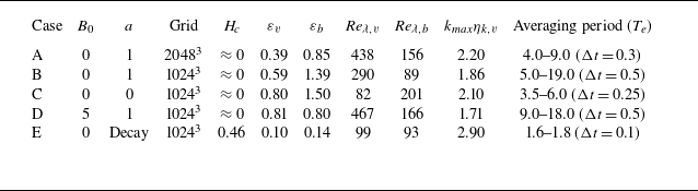
 B0
 a
 Hc
 εv=ν∑kk2⟨|u^(k,t)|2⟩
 εb=η∑kk2⟨|b^(k,t)|2⟩
 Reλ,u=urmsλu/ν
 Reλ,b=urmsλb/η
 λu=15νurms2/εu
 λb=15ηbrms2/εb
 urms=⟨|u|2/3⟩
 brms=⟨|b|2/3⟩
 ηk,v
 kmax
 Te=Lv/urms
 Lv=3π/4[∑kk−1Ev(k)]/Ev
 Ev=∑kEv(k)
 tstart−tend
 Δt
 Δt
 Δt=0.3
 4.0Te
 9.0Te
 0.3Te

 k5/3
 k3/2
 k5/3
 k−3/2
 k−5/3
 r∗=r/ηk,v
 5%
 1

 ε¯+
 y
 r∗=r/ηk,v
 r∗=2
 243
 25≲r∗≲95
 B0=0
 20483

 εr+
 εr+
 sr+=(lnεr+−mr+)/σr+
 mr+=⟨lnεr+⟩
 σr+=⟨(lnεr+−mr+)2⟩
 r∗
 r∗=2
 r∗=243
 25≲r∗≲95
 α+
 εr+
 εr+

 r
 r
 sr+≈[−4.5,4.5]
 sr+
 r
 θ+
 r

 (Rer+)1/2
 Rer+
 Ur+=(rεr+)1/3

 β1+=|δz∥+|/Ur+
 β2+=|V+|/Ur+
 sr+
 r∗≈
 Rer+

 εr+
 B0=0
 20483

 β1+=|δz∥+|/Ur+
 β2+=|V+|/Ur+
 Rer+≈
 r
 εr+
 f(β1±)
 f(β2±)
 β1±
 β2±

 Rer+
 εr+
 Rer+≈[80,1200]
 Rer+≈[100,600]

 n
 Dn
 Dn
 Dn′
 Dn′
 B0=0
 20483

 Rer+
 r∗∈[2,223]
 B0=0
 3
 r∗≈[30,90]
 r∗≈[10,50]
 B0=5
 r∗≈[30,90]

 Rer±
 z+
 z−
 B0=0
 3
 Hc=0.46
 r∗≈[10,15]
 r∗≈[1,97]

 Rer+
 V⊥±=(δz⊥∓(δz±)2)1/3
 3
 B0=0

 x,y,z
 Rer+
 2563
 B0=0


