INTRODUCTION
In livestock production, the stockman's management aims at generating long-term profitability of the farm by efficiently producing as much milk, eggs or meat as possible with the desired quality to meet the customers’ and consumers’ demands (Frost et al. Reference Frost, Schofield, Beaulah, Mottram, Lines and Wathes1997; Mertens et al. Reference Mertens, De Ketelaere, Vaesen, Löffel, Ostyn, Kemps, Kamers, Bamelis, Zoons, Darius, Decuypere and De Baerdemaeker2008). This farm management comprises the stockman's skill, experience and assessment capability to oversee and interpret the livestock production process and take decisions to achieve an optimal ratio between the production value and production costs (Lokhorst Reference Lokhorst1996). Most stockmen recognize the need for monitoring and controlling livestock performance, and yet few of them know how to do it in an effective way (Dohoo Reference Dohoo1993; Polson et al. Reference Polson, Baum and Holck1999).
In addition to the efforts for improving the general production process in a profitable way, the timely signalling of undesired performance changes is another important challenge for day-to-day livestock management. This is required in order to keep results within a desired predefined range and reduce economic loss (Huirne Reference Huirne1990). It requires the continuous monitoring of animal health, welfare and production performance, which in turn calls for recording of several process parameters on a regular basis. Precision livestock farming (PLF) is a relatively new discipline that originated from the increased use of information technology (IT) products in support of livestock management (Banhazi et al. Reference Banhazi, Dunn, Cook, Black, Durack, Johnnson and Cox2007). One of the main aims of PLF is the development of sensors that measure the most important process parameters of the different livestock production systems more accurately, continuously and automatically (Wathes et al. Reference Wathes, Kristensen, Aerts and Berckmans2008).
These sensors provide the stockman with ample detailed information, giving him/her more insight into the livestock production process (Frost et al. Reference Frost, Schofield, Beaulah, Mottram, Lines and Wathes1997). Yet, use of this information for improving management in current livestock production practice is still rather limited. These data are seldom analysed statistically, leading to doubt in the interpretation of data (Noordhuizen et al. Reference Noordhuizen, Frankena, Stassen, Brand and Williams1992; Thysen Reference Thysen1993). As a consequence, good and successful management of most livestock production processes still depends largely on the skill, experience and assessment capability of the stockman to oversee and interpret the daily variation in the recorded data flows. It is precisely the lack of understanding of the information captured in the variation of the process parameters which forms the main problem in the management of production processes (Deming Reference Deming1986). In addition, the increasing complexity of livestock production has led to a considerable reduction in the time available to the stockman for observing animals and interacting with them (Wrathall & Hebert Reference Wrathall and Hebert1982; Frost et al. Reference Frost, Schofield, Beaulah, Mottram, Lines and Wathes1997), which complicates management decisions even more.
Because financial results depend heavily on management and complex decision situations (Ziggers & Bots Reference Ziggers, Bots, Christensen, Rasmussen and Stryg1989), it is clear that there is a need for fact-based information to improve the quality of the day-to-day management decisions (Reneau & Lukas Reference Reneau and Lukas2006). The development of integrated systems managing both the biological and the physical processes of livestock production is necessary to fully exploit the available data (Wathes et al. Reference Wathes, Kristensen, Aerts and Berckmans2008).
The availability of regularly recorded data on the variables of the livestock production processes creates the opportunity to develop control charts, a well-known tool of statistical process control (SPC), to support the stockman in his daily management tasks. Basically, a control chart is a graphical representation of the observations of a certain process variable against the measurement time and with limits between which the variable is allowed to vary. If an observation crosses these limits, an alarm is given, indicating that there is a problem. The main objective of control charts is to support understanding of the information in process variation (Deming Reference Deming1986) and to make a distinction between normal and abnormal variation (Montgomery Reference Montgomery2009). The graphical basis of control charts provides a comprehensible performance picture (Wrathall & Hebert Reference Wrathall and Hebert1982).
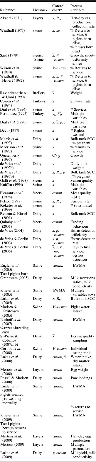
In industrial production (automotive, chemical, …), the concepts of SPC and more specifically control charts have already been used as part of quality assurance programmes for many years. The use of control charts in livestock production is gaining interest. Based on the work of de Vries (Reference de Vries2001) and Reneau & Lukas (Reference Reneau and Lukas2006), and further extended with more recent literature, Table 1 lists the most important papers published in this field.
Overview of publications applying control charts to data from livestock production systems

* Control chart:x: Shewhart chart for individual observations;  : Shewhart chart for mean of subgroups; s: Shewhart chart for standard deviation; s 2: Shewhart chart for variance; p: Shewhart chart for probability of success; R m: Shewhart chart for moving range; cusum: algorithmic cumulative sum chart; V–cusum: V-mask cusum; EWMA: exponentially moving average chart; cusum, Q: Q-chart for mean; s Q2: Q-chart for variance; CVQ: Q-chart for coefficient of variation. SCC=somatic cell count.
The fact that about half of the papers in Table 1 were published within the last decade provides proof of the increasing interest in this area. Control charts have been applied to the most important sectors of livestock production, and yet the majority of the papers were on dairy and pig (mainly sows) production data. Fewer papers presented an application in poultry (layers, turkeys and broilers) and beef cattle.
The rationale of the majority of publications is to use control charts as a support tool for the decision-making process of the stockman, focusing on one or more process variables and designing a control chart for them. Some of the papers in Table 1 used control charts as a mean to perform the statistical analysis of specific experimental data. Koketsu et al. (Reference Koketsu, Duangkaew, Dial and Reeves1999) analysed the within-farm variability in the number of sows mated per week. Krieter et al. (Reference Krieter, Kirchner, Engler and Tölle2005) performed an on-farm sow herd performance analysis by comparing it with a fixed standard. St-Pierre & Cobanov (Reference St-Pierre and Cobanov2007a, Reference St-Pierre and Cobanovb) used a control chart as a means of defining the optimal sampling scheme for the nutritional value of forages. Galli et al. (Reference Galli, Signori and Balduzzi1998) used a control chart to optimize the number of forward spermatozoa in bovine semen straws.
The scope of the present review is to discuss the most important aspects, recommendations, pitfalls and opportunities for the development of control charts and for the evaluation of their performance when applied to livestock process data. Firstly, some basics for control charting are presented. Then there follows a brief discussion on the dynamic aspects of data originating from livestock production processes. In the subsequent sections, the main control chart aspects – data collection, choice of control chart, chart construction and chart performance – are discussed, referring to the reviewed papers. Finally, a promising approach for dealing with the dynamic aspects of livestock process data and the importance of real-time monitoring is discussed before concluding with a more general discussion. The strategies and results of the reviewed papers related to these aspects will be referred to in the respective sections.
STATISTICAL CONTROL CHARTS
Variability is a phenomenon innate to every single production process and, regardless of the process design or maintenance, it is unavoidable. The quality level of products is directly related to the process variability. Two kinds of process variability can be discerned: the common cause or expected (innate) variation and the special cause or unexpected variation (Shewhart Reference Shewhart1931). Special causes in livestock production may occur as a result of human error, technical failures, contamination of feed or water, health problems, etc. A production system that shows only expected variation is said to be statistically in control and when a special cause gives rise to an altered process performance (process shift), resulting in inferior product quality, the process is statistically out of control (DeVor et al. Reference DeVor, Chang and Sutherland1992; Wadsworth et al. Reference Wadsworth, Stephens and Godfrey2002; Montgomery Reference Montgomery2009). Hence, the basis of quality control is the understanding of the information contained in process variability (Deming Reference Deming1986). The concepts of SPC have been designed for this purpose.
Essentially, SPC is a collection of tools that aims to detect the occurrence of process shifts as a result of special causes. Control charts are SPC tools that enable visualization and detection of process shifts. The limits of the control charts are formulated based on the common cause of variation of the considered process or quality parameter. When the process is in control, nearly all measurements will fall within the range of the control limits and hence most likely within expected random variability. Any problem which causes unexpected process variation, i.e. the special cause variation, results in control chart recordings outside of its limits. At that moment, investigation is required to identify the cause and corrective measures are required in order to resolve the problem. As such, control charts are useful tools for achieving process stability through a reduction of variability (DeVor et al. Reference DeVor, Chang and Sutherland1992; Wadsworth et al. Reference Wadsworth, Stephens and Godfrey2002; Montgomery Reference Montgomery2009).
Since control charts are related to repeated hypothesis testing and hence probability calculations, two types of signalling errors can be made. A Type I error – false alarm or false positive – occurs when the chart produces a signal without a change of the process. A Type II error – false negative – is made when the chart generates no signal in spite of a process change. The rates of these errors depend on the setting of the control limits. The narrower the control limits, the more sensitive the chart (fewer Type II errors) and yet the more false alarms (Type I error).
Performance measures of control charts are based on the frequency of Type I and II errors, expressed in terms of run lengths, i.e. the number of observations between a certain starting observation and an observation which causes an alarm. The average run length (ARL) is often used for summarizing chart performance. The in-control ARL (ARL0) measures the in control behaviour and hence indicates the average time between false alarms (Type I errors). The ARL0 should be relatively long: false alarms are obviously undesirable as they waste time and energy and disrupt operations looking for non-existent special causes (Wieringa Reference Wieringa1999). The out of control ARL (ARL1) is the average ARL until an alarm is given after a shift of the process. Hence, it indicates the speed of detection and should be as short as possible.
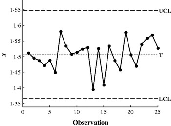
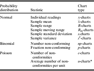
A wide range of control charts has been developed for different types of data and for a desired size of the detectable shift. The first and probably best-known control chart was introduced by Shewhart (Reference Shewhart1931). The Shewhart control chart is typically used to detect large shifts (>3 sigma (σ)). Shewhart charts have been developed for all well-known probability distributions (Table 2). A typical example of a Shewhart control chart is given in Fig. 1. However, the classical Shewhart charts require a specification of the process mean and variance before charting. Quesenberry introduced Q-charts for most statistical measures and probability distributions partly to address these limitations (Quesenberry Reference Quesenberry1991, Reference Quesenberry1995, Reference Quesenberry1997). Basically, Q-charts transform original observations into a normally distributed data series with zero mean and unit variance. These Q-charts are useful for short runs in which process mean and variance are unknown (Quesenberry Reference Quesenberry1991, Reference Quesenberry1995, Reference Quesenberry1997).
Example of a typical control chart. T=target (process mean); UCL/LCL=upper/lower control limit=T± 3σ. Figure based on data from Montgomery (Reference Montgomery2009), p. 200.

Overview of the different types of Shewhart charts for different probability distributions

* u=c/n.
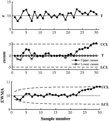
Shewhart charts have no ‘memory’, meaning that they only use the information of the current measurement. Although they are often supplemented with ‘run rules’, they have not proved to be very sensitive for small shifts (<1·5σ); therefore, other types of control charts, which make use of the information in the previous measurements, have been designed to detect these. The cumulative sum (cusum) chart introduced by Page (Reference Page1954) and the exponentially weighted moving average (EWMA) chart introduced by Roberts (Reference Roberts1959) are typical ‘memorizing’ control charts that are more successful in detecting small shifts, which are particularly of interest in biological processes. These charts are also developed for all well-known probability distributions. The EWMA and cusum charts have comparable performance results for detecting small shifts. The cusum chart is usually a little faster in detecting step changes, while the EWMA is less fit for estimation after the step change has occurred. In addition, the cusum control scheme has the possibility to return to zero. The EWMA chart gives an immediate estimate of the current process mean, while the cusum needs some calculation to determine this (Hawkins & Olwell Reference Hawkins and Olwell1998; de Vargas et al. Reference de Vargas, Lopes and Souza2004; Montgomery Reference Montgomery2009). Making a choice between these two charts depends on the process for which control charts have to be designed. Examples of a cusum chart and an EWMA chart are given in Fig. 2b and c. For more detailed information on the different control charts and statistical and technical concepts for control chart construction, the SPC text books by DeVor et al. (Reference DeVor, Chang and Sutherland1992), Wadsworth et al. (Reference Wadsworth, Stephens and Godfrey2002) and especially Montgomery (Reference Montgomery2009) are highly recommended.
(a) Example data taken from Montgomery (Reference Montgomery2009), p. 387. (b) Example of a cusum control chart and (c) of an EWMA control chart for a shift in normal mean, based on (a). The first 20 observations are drawn from a normal distribution N(10, 1), the last 10 observations come from a normal distribution N(11, 1), and so a shift of 1σ occurred. The cusum control scheme was designed to detect a shift of 1σ with reference value k=0·5 and control limit H=5. The cusum chart generates an alarm at observation 29 (C+>H). The parameters of the EWMA control chart are the weighting factor λ, which defines how much weight is set on previous observations, and the control limit L. The settings for these parameters in this example are, respectively, λ=0·10 and L=2·7. The EWMA chart generates an alarm at observation 29 (z29>UCL). T=target (process mean); UCL/LCL=upper/lower control limit.

The proper use of control charts requires several assumptions about the model underlying the process. The chart calculations are derived based on these assumptions. The first assumption states that the data generated by the in-control state of the production process must be stationary. A time series is said to be stationary when its statistical properties, mean and (co)variance, are not affected in time and hence the probability distribution is the same for all time periods. The second assumption is on the statistical serial independence of consecutive process recordings. In serial dependence, often expressed in terms of autocorrelation, consecutive recordings are strongly correlated, either positively or negatively. The third assumption is that the data follow the statistical distribution function associated with the specific control chart (normal, binomial, chi-square, Poisson, etc.) (Montgomery et al. Reference Montgomery, Jennings and Kulahci2008; Montgomery Reference Montgomery2009). If all assumptions hold exactly for the considered data, the performance of SPC charts can be exactly determined. Unfortunately, this is not usually the case (Montgomery Reference Montgomery2009), especially for livestock process data. Assumption violations in livestock data are the result of the dynamic aspects of these data. Ignoring assumption violations dramatically compromises control chart performance, especially in case of non-stationarity and autocorrelation. The next section discusses the assumption issues of raw livestock production data.
DYNAMIC ASPECTS OF LIVESTOCK PROCESS DATA
The biological character of livestock production processes is reflected in the data collected from these processes. Typically, biological data are seldom stationary and hence have no fixed target value, and they mostly display autocorrelation between successive observations. Furthermore, in many cases biological data series contain missing values as a result of, for instance, technical failure or (either deliberate or unintentional) managerial error. From a statistical point of view, the assumptions usually made about industrial process data are often invalid for biological process data, which complicates the direct application of control charts for these data.
These peculiarities are a result of the fact that many parameters of livestock production processes are subjected to systematic variation caused by, e.g. the age of the animals or seasonal fluctuations (Sard Reference Sard1979). The most dominant driver behind such age-dependent dynamics are of physiological origin and are primarily related to animal growth or to a change of functionality of producing organs, e.g. pig muscle growth in time, chicken ovary development in time and cow milk gland functionality in different lactation phases and numbers.
Mertens et al. (Reference Mertens, De Ketelaere, Vaesen, Löffel, Ostyn, Kemps, Kamers, Bamelis, Zoons, Darius, Decuypere and De Baerdemaeker2008, Reference Mertens, Vaesen, Löffel, Kemps, Kamers, Zoons, Darius, Decuypere, De Baerdemaeker and De Ketelaere2009) and Mertens (Reference Mertens2009) show that for chickens, all process parameters (except for mortality) of layer production show a dynamic deterministic trend as a function of age (growth to physical and sexual maturity) of the hens. In dairy cows, de Vries et al. (Reference de Vries, Conlin, Marsh and Reneau1997a) and Lukas et al. (Reference Lukas, Reneau, Wallace, Hawkins and Munoz-Zanzi2009) consider the trend in daily milk yield as a result of the stage of lactation and the lactation number. Lukas et al. (Reference Lukas, Reneau, Wallace, Hawkins and Munoz-Zanzi2009) also indicated that milk electrical conductivity increases as a function of lactation stage and lactation number. Lukas et al. (Reference Lukas, Reneau and Linn2008) talk about the ‘drift’ in the dry matter intake of dairy cows as lactation progresses. In growing pigs, Madsen & Kristensen (Reference Madsen and Kristensen2005) mentioned a daily circadian rhythm and an increasing dynamic trend in water consumption with age. Modelling of day-to-day dynamic trends in livestock process data has been discussed by, amongst others, Lokhorst (Reference Lokhorst1996) for laying hens, Bebbington et al. (Reference Bebbington, Lai and Zitikis2009) and Silvestre et al. (Reference Silvestre, Martins, Santos, Ginja and Colaço2009) for lactation curves of dairy cows, Darmani-Kuhi et al. (Reference Darmani-Kuhi, Kebreab, Lopez and France2003) for broiler growth and Emmans & Kyriazakis (Reference Emmans and Kyriazakis1997) for pig growth.
Mertens et al. (Reference Mertens, De Ketelaere, Vaesen, Löffel, Ostyn, Kemps, Kamers, Bamelis, Zoons, Darius, Decuypere and De Baerdemaeker2008, Reference Mertens, Vaesen, Löffel, Kemps, Kamers, Zoons, Darius, Decuypere, De Baerdemaeker and De Ketelaere2009) and Mertens (Reference Mertens2009) also discuss the occurrence of missing values in their layer data. While this issue is less important for control chart calculations, it becomes a problem for estimating the coefficients of models, such as time series models, used to handle the other aforementioned data issues. The problem becomes even more complex in the case of multivariate control charting. Since Mertens et al. (Reference Mertens, De Ketelaere, Vaesen, Löffel, Ostyn, Kemps, Kamers, Bamelis, Zoons, Darius, Decuypere and De Baerdemaeker2008, Reference Mertens, Vaesen, Löffel, Kemps, Kamers, Zoons, Darius, Decuypere, De Baerdemaeker and De Ketelaere2009) and Mertens (Reference Mertens2009) are the only authors discussing this issue, the current review abstains from an in-depth discussion of this problem.
The dynamic aspects of biological production data impede the direct application and use of classical control charts, mainly because of poor chart performance (see section on Synergistic Control). As a result, the use of this methodology in agricultural production and, more specifically, livestock production is rather limited when compared with industrial production. Nevertheless, the approach has gained interest in recent years, and proper pre-processing of the data will account for the dynamic aspects of livestock process data.
In the following sections, the main control chart aspects – data collection, choice of control chart, chart construction and chart performance – are discussed. The publications included were screened for these aspects and reference is made to the appearance of the aforementioned aspects in the cited papers.
DATA COLLECTION
Practical relevance of the process parameter
The first question raised is which process parameter is the more interesting to use for process monitoring. Initially, the recorded data series of parameters should be sensitive to process changes, independent of whether these originate from diseases, technical failures or management errors (DeVor et al. Reference DeVor, Chang and Sutherland1992; Wadsworth et al. Reference Wadsworth, Stephens and Godfrey2002; Montgomery Reference Montgomery2009).
When the main aim of the process monitoring is to safeguard animal health, the most important criterion should be how well the physiological balance of the animals is reflected in a process parameter. The physiological status is the basis for a good health status and good production performance. Two of the most critical and highest physiologically related parameters are feed and water consumption, which can be either monitored directly (Madsen & Kristensen Reference Madsen and Kristensen2005; Lukas et al. Reference Lukas, Reneau and Linn2008; Mertens Reference Mertens2009) or indirectly through feeding behaviour (Quimby et al. Reference Quimby, Sowell, Bowman, Branine, Hubbert and Sherwood2001) or eating hierarchy (Cornou et al. Reference Cornou, Vinther and Kristensen2008). Performance parameters closely related to consumption are body weight (muscle mass) and body weight gain (muscle growth) (Sard Reference Sard1979; Ravindranathan & Unni Reference Ravindranathan and Unni1990; Quesenberry Reference Quesenberry1997). Another approach for monitoring animal health is the direct or indirect monitoring of specific health problems (Sard Reference Sard1979; de Vries et al. Reference de Vries, Conlin, Reneau, Kinsel and Marsh1997b; Marsh et al. Reference Marsh, de Vries, Reneau and Kinsel1997; Reneau & Kinsel Reference Reneau, Kinsel and Radostits2001; Grennstam Reference Grennstam2005; Lukas et al. Reference Lukas, Hawkins, Kinsel and Reneau2005; Pastell & Madsen Reference Pastell and Madsen2008).
The majority of the papers handle economically relevant parameters related to animal fertility (Wrathall Reference Wrathall1977; Wilson et al. Reference Wilson, McMillan and Swaminathan1980; Wrathall & Hebert Reference Wrathall and Hebert1982; Dial et al. Reference Dial, Duangkaew, Rademacher and Allen1996, Reference Dial, FitzSimmons, BeVier, Wiseman and Allen1994; de Vries et al. Reference de Vries, Conlin, Marsh and Reneau1997a, Reference de Vries, Conlin, Reneau, Kinsel and Marshb; Deen Reference Deen1997; Marsh et al. Reference Marsh, de Vries, Reneau and Kinsel1997; Morrison et al. Reference Morrison, Dial, Bahnson, Marsh, Collins, Polson and Youngquist1997; Polson Reference Polson1998; de Vries Reference de Vries2001; de Vries & Conlin Reference de Vries and Conlin2003, Reference de Vries and Conlin2005; Engler et al. Reference Engler, Tölle, Timm, Hohls, Krieter and Cox2005, Reference Engler, Tölle, Timm, Hohls and Krieter2009; Niehoff et al. Reference Niehoff, Tölle and Krieter2007; Krieter et al. Reference Krieter, Engler, Tölle, Timm and Hohls2009) and to production performance or product quality (Akachi Reference Akachi1971; de Vries et al. Reference de Vries, Conlin, Marsh and Reneau1997a; Pleasants et al. Reference Pleasants, McCall and Sheath1998; Grennstam Reference Grennstam2005; Mertens et al. Reference Mertens, De Ketelaere, Vaesen, Löffel, Ostyn, Kemps, Kamers, Bamelis, Zoons, Darius, Decuypere and De Baerdemaeker2008, Reference Mertens, Vaesen, Löffel, Kemps, Kamers, Zoons, Darius, Decuypere, De Baerdemaeker and De Ketelaere2009; Lukas et al. Reference Lukas, Reneau, Wallace, Hawkins and Munoz-Zanzi2009). Parameters that reflect collective production or quality performance, such as hen-day egg production in laying hens, are less sensitive to process changes as they pool the inter-individual variability. However, control charts of these parameters are of interest because they provide relevant information on the production aspect of the highest value for the stockman, because they generate the financial return. The development of control charts for production and quality parameters becomes more valuable when information from each animal (e.g. milk production of each cow) or each product (e.g. each egg, milk at each milking service) is available. The variability in quality between each measurement unit, albeit animal or product, holds valuable information for optimizing total process output and product quality. Control charts for variability can therefore be valuable tools.
Few authors provide a discussion on the choice of process parameters. In most cases the choice for parameters is practically driven – ‘used in practice’ or ‘suggested to be used as management aids’ (de Vries & Conlin Reference de Vries and Conlin2003) – or economically driven – ‘a very important impact factor for the economy of the herd’ (Niehoff et al. Reference Niehoff, Tölle and Krieter2007) – and such choices result in parameters that are related to main issues such as fertility in sows and dairy, or growth in grower pigs, beef cattle and broilers. Only Krieter et al. (Reference Krieter, Kirchner, Engler and Tölle2005) perform a thorough analysis of several sow farm data sets, using a weighting principle based on statistical and economical aspects to make a ranking in process parameters. Wrathall (Reference Wrathall1977) mentions the impact on overall performance in his choice and states that the parameters should be able to signal a problem quickly. Madsen & Kristensen (Reference Madsen and Kristensen2005) state that eating and drinking patterns are strongly related to animal well-being and health. Galli et al. (Reference Galli, Signori and Balduzzi1998) explain their choice of parameters on semen quality by stating that these parameters have the best correlation with on-farm assessments. Pastell & Madsen (Reference Pastell and Madsen2008), when setting up a new system for lameness detection, stated that paw loading recordings are more objective than current visual inspection methods, which fail to recognize up to 0·75 of the cases. Lukas et al. (Reference Lukas, Reneau and Linn2008) indicated that water and dry matter intake are quickly and often strongly influenced by various health disorders. Other authors develop charts for almost all interesting and frequently measurable parameters (Kniffen Reference Kniffen and Allen1994; Fernandez Reference Fernandez1995; Dial et al. Reference Dial, Duangkaew, Rademacher and Allen1996; Krieter et al. Reference Krieter, Kirchner, Engler and Tölle2005; Mertens Reference Mertens2009).
Measurement frequency and rational subgrouping
Besides the aspect of physiological or economic relevance of parameters, it must be possible to record the data frequently to provide the stockman with timely feedback (Reneau & Lukas Reference Reneau and Lukas2006). For instance, data on water or feed consumption of a pen of pigs can be registered in real time, while the success of insemination of cows can only be detected after about 21 days. In the latter case, the economic relevance of the parameter supports its usefulness, as long as the control charts are well designed.
An important issue related to the frequency of data collection is the formation of rational subgroups. Although many authors use individual measurements, the use of rational subgroups is advisable in most cases. Rational subgrouping can reduce the measurement frequency and reduce dependence between subsequent measurements. A rational subgroup is a set of observations generated under highly similar conditions (de Vries Reference de Vries2001). The sample size of the rational subgroups is important (Wadsworth et al. Reference Wadsworth, Stephens and Godfrey2002) and requires thorough process knowledge. The main consideration in sample size selection is often practically related. Depending on the parameter that has to be monitored, it might be possible to collect more observations at the same time or closely after each other in a certain period. For example, in egg production it is possible to measure the individual egg weight on a sample of a day's production. Wadsworth et al. (Reference Wadsworth, Stephens and Godfrey2002) and Montgomery (Reference Montgomery2009) indicated that the time order of data is mostly a good basis for forming subgroups since it allows the detection of shifts occurring over time. This is confirmed in papers by Reneau & Kinsel (Reference Reneau, Kinsel and Radostits2001) and Reneau & Lukas (Reference Reneau and Lukas2006). Wheeler (Reference Wheeler1995) states that rational sampling and subgrouping is essential for effective control chart application.
Few papers have paid attention to rational subgrouping and those that have mostly chosen practically convenient sampling methods, using all data for a fixed period of time. Encountered subgroups were pooled per hour, day, week, or month or complete production period. In most cases, sample sizes were variable. Dial et al. (Reference Dial, Duangkaew, Rademacher and Allen1996) paid attention to time of sampling and sampling frequency in relation to the ability of detection by Shewhart charts. For the prediction of drinking behaviour, Madsen & Kristensen (Reference Madsen and Kristensen2005) have a sampling frequency of 2 min, which yields data dominated by random noise, which was reduced by aggregating the 2-min recordings into 1-h intervals. This was also true for Quimby et al. (Reference Quimby, Sowell, Bowman, Branine, Hubbert and Sherwood2001), who aggregated their sampled data (every 5 s) into 3-h intervals.
Both the frequency of data collection and the rational subgrouping have important consequences on the statistical characteristics of the collected data series and hence on the choice of the control chart. This is discussed in the next section.
CHOICE OF THE CONTROL CHART
The choice of the control chart should be based on two criteria. The first is the size of the desired shift to detect: larger shifts use Shewhart charts, while smaller shift detections are performed using cusum and EWMA charts. The second criterion is related to the statistical characteristics of the data. For instance, proportions are assumed to be binomially distributed and hence p-charts or binomial cusum or EWMA charts are used.
In some cases it can be questioned as to whether the control chart used is the most suitable for the considered process parameter. For instance, in the case of large sample sizes, the distribution of proportional data approaches the normal distribution. Such issues can be studied through simulation. de Vries & Conlin (Reference de Vries and Conlin2003, Reference de Vries and Conlin2005) investigated both the binomial and the normal distribution for proportional parameters. They suggest that the normal distribution is appropriate for proportions when the size n of the subgroup is large enough (>20) and found that the performance of x-charts and p-charts, and the normal and binomial cusum on the same proportional data, were similar.
The availability of extra information may lead to the addition of an extra chart. The possibility of rational subgrouping provides variability information within samples and hence enables the use of control charts for variability (R-, R m-, s- and s 2-charts). Differences between samples indicate a shift in the process parameter (control charts for mean), differences within samples indicate inherent variability (control charts for variability).
Some papers discuss how to choose the most suitable control chart, several dealing with the choice between the cusum and EWMA chart. Both charts have comparable performance results on detecting small shifts (de Vargas et al. Reference de Vargas, Lopes and Souza2004), but the cusum chart is usually slightly faster in detecting step changes while the EWMA is less fit for estimation after the step change has occurred (Hawkins & Olwell Reference Hawkins and Olwell1998; Montgomery Reference Montgomery2009). Practical considerations are often mentioned when considering the choice between cusum and EWMA. Engler et al. (Reference Engler, Tölle, Timm, Hohls and Krieter2009) choose the cusum because it is more straightforward and the settings are easier to handle. Krieter et al. (Reference Krieter, Engler, Tölle, Timm and Hohls2009) consider that the EWMA may be easier to understand since actual values are assigned, namely an estimate of the current process mean (Montgomery Reference Montgomery2009), in contrast to the cusum, which works with deviations. But Krieter et al. (Reference Krieter, Engler, Tölle, Timm and Hohls2009) also state that the cusum has the possibility to differentiate between positive and negative deviations. In the framework of his work, Mertens (Reference Mertens2009) chooses the cusum control scheme because it has the possibility to quickly return to zero. Lukas et al. (Reference Lukas, Reneau, Wallace, Hawkins and Munoz-Zanzi2009) use a combination of the Shewhart chart and the cusum chart for good detection of both large and small process shifts. This is also advised by DeVor et al. (Reference DeVor, Chang and Sutherland1992), Hawkins & Olwell (Reference Hawkins and Olwell1998) and Montgomery (Reference Montgomery2009).
Some papers use the V-mask type of cusum, a graphical alternative to the more frequently used algorithmic cusum mentioned earlier. For more information concerning this V-mask cusum, refer to Montgomery (Reference Montgomery2009), who strongly advises against the use of the V-mask procedure, mainly because of statistical issues in the choice of the false alarm rate. Sard (Reference Sard1979), Wilson et al. (Reference Wilson, McMillan and Swaminathan1980) and Wrathall & Hebert (Reference Wrathall and Hebert1982) use a V-mask cusum for snout-deformity scores in pigs, percent return to service and number of piglets born alive. Madsen & Kristensen (Reference Madsen and Kristensen2005) and Cornou et al. (Reference Cornou, Vinther and Kristensen2008) use a V-mask cusum for detecting estrus and health problems in sows. Madsen & Kristensen (Reference Madsen and Kristensen2005) suggest the use of the V-mask as a tool for discriminating between the age-dependent trend in the data as a result of the pigs growing and changes due to sudden problems such as disease outbreaks. The long-term, age-dependent cusum drift can indeed be taken into account by the V-mask; nevertheless, it is an arbitrary setting of tolerated age-related dynamics. Madsen & Kristensen (Reference Madsen and Kristensen2005) partly try to overcome this issue by standardizing the data used.
The actual investigation of compliance with the model assumptions underlying the control charts is easily overlooked by most authors. Some papers mention the probability distribution assumption. de Vries et al. (Reference de Vries, Conlin, Reneau, Kinsel and Marsh1997b) (bulk tank somatic cell count) and Engler et al. (Reference Engler, Tölle, Timm, Hohls, Krieter and Cox2005) and Krieter et al. (Reference Krieter, Engler, Tölle, Timm and Hohls2009) (total piglets born) refer to other papers that provide proof of the normal distribution for their parameters. Only Mertens (Reference Mertens2009) and Mertens et al. (Reference Mertens, Vaesen, Löffel, Kemps, Kamers, Zoons, Darius, Decuypere, De Baerdemaeker and De Ketelaere2009) graphically analyse their raw data for assumption violations prior to control chart design, and found violations of the stationarity and independence assumptions in layer data. de Vries et al. (Reference de Vries, Conlin, Marsh and Reneau1997a) acknowledge the issue of non-stationarity in daily milk weight. Krieter et al. (Reference Krieter, Kirchner, Engler and Tölle2005, Reference Krieter, Engler, Tölle, Timm and Hohls2009) mention the problem of serial correlation, indicating that it has to be removed before the application of control charts. Lukas et al. (Reference Lukas, Reneau and Linn2008, Reference Lukas, Reneau, Wallace, Hawkins and Munoz-Zanzi2009) indicated the presence of non-stationarity and autocorrelation in their data. Madsen & Kristensen (Reference Madsen and Kristensen2005) and Cornou et al. (Reference Cornou, Vinther and Kristensen2008) acknowledge that the systematic variation on top of the random variation complicates the application of SPC techniques in their hourly water consumption data.
Most of the aforementioned authors provide some solution to solve the issue of assumption violations. A detailed discussion on this is provided in the section on Synergistic Control.
Control charts are especially sensitive to the first two assumptions (stationarity and independence). Their degree of (in)sensitivity is referred to as ‘chart robustness’. This robustness can be expressed in terms of the performance measures, ARL0 and ARL1. The performance (e.g. ARL0) of a non-robust control chart in response to violating data will be a strong deviation from the expected performance (more false alarms, smaller ARL0). Borror et al. (Reference Borror, Montgomery and Runger1999) state that the Shewhart chart is very sensitive to non-normality. However, Woodall (Reference Woodall2000) questions the importance of distribution robustness on practical applications. Indeed, Montgomery (Reference Montgomery2009) states that the EWMA is very insensitive to the normality assumption since it is a weighted average of all past and current observations, and that the cusum is less robust than EWMA for violations of the normality assumption. However, Hawkins & Olwell (Reference Hawkins and Olwell1998) state that the impact of non-normality on the performance of a cusum chart depends on size of the shift for which the chart is tuned. They found that the effect of non-normality is greatest when the cusum is tuned to detect large shifts (large k and h). Wieringa (Reference Wieringa1999) shows that the serial autocorrelation (often also resulting in non-stationarity) has a strong influence on performance of the Shewhart, cusum and EWMA chart, which was confirmed by del Hawkins & Olwell (Reference Hawkins and Olwell1998), del Castillo (Reference del Castillo2002) and Montgomery (Reference Montgomery2009).
Few papers mention chart robustness. Based on simulations, de Vries & Conlin (Reference de Vries and Conlin2003, Reference de Vries and Conlin2005) found that both Shewhart and cusum charts are rather dependent on the goodness of fit of the assumed probability distribution model. Sard (Reference Sard1979) says that his cusum chart is fairly robust to the normality assumption, and yet does not present proof.
CHART CONSTRUCTION
The construction of control charts consists of two phases. Phase I could be considered as the calibration phase. The process is explored and recursively purified of out-of-control observations to obtain in-control process data. Next, the parameters required for setting up the control chart target (process mean) and limits, used for monitoring in Phase II, are estimated.
Phase I has to be long enough, because a higher difference between the true values of statistical measures (μ, σ) and their estimates (, s) could have a large effect on control chart performance (Quesenberry Reference Quesenberry1997). However, this depends on the chart type: for instance, cusum charts are more sensitive to such errors than Shewhart charts (Hawkins & Olwell Reference Hawkins and Olwell1998). It is recommended that at least 25–30 subgroups of a minimum of five observations are available to obtain reliable estimates of the in control process. However, procedures for short-run processes and processes where quick monitoring is necessary, which is in particular of interest for livestock processes, have been proposed (Quesenberry Reference Quesenberry1997; Hawkins & Olwell Reference Hawkins and Olwell1998; Montgomery Reference Montgomery2009).
Only a few papers mention the application of the two phases explicitly when designing their charts. Pastell & Madsen (Reference Pastell and Madsen2008), Mertens et al. (Reference Mertens, De Ketelaere, Vaesen, Löffel, Ostyn, Kemps, Kamers, Bamelis, Zoons, Darius, Decuypere and De Baerdemaeker2008, Reference Mertens, Vaesen, Löffel, Kemps, Kamers, Zoons, Darius, Decuypere, De Baerdemaeker and De Ketelaere2009) and Mertens (Reference Mertens2009) describe the procedure of control chart construction in the two phases. Pastell & Madsen (Reference Pastell and Madsen2008) use c. 40 observations (10–20 days) as Phase I to estimate in control variation, while Mertens et al. (Reference Mertens, De Ketelaere, Vaesen, Löffel, Ostyn, Kemps, Kamers, Bamelis, Zoons, Darius, Decuypere and De Baerdemaeker2008, Reference Mertens, Vaesen, Löffel, Kemps, Kamers, Zoons, Darius, Decuypere, De Baerdemaeker and De Ketelaere2009) and Mertens (Reference Mertens2009) take 40 and 21 days for Phase I. de Vries & Conlin (Reference de Vries and Conlin2003, Reference de Vries and Conlin2005) describe the difference between Phase I and Phase II in their study. Galli et al. (Reference Galli, Signori and Balduzzi1998) mention Phase I and Phase II, but it is not clear whether they actually performed the steps. Cornou et al. (Reference Cornou, Vinther and Kristensen2008) talk about a reference period for chart estimation, and yet Phase I is not mentioned and no purification sequence is performed. Lukas et al. (Reference Lukas, Reneau, Wallace, Hawkins and Munoz-Zanzi2009) use historical data to construct a head-start control chart.
Considerations on control chart calibration in Phase I
The control limits of a control chart are the ‘decision makers’ and setting of the control limits is crucial for chart performance. The narrower are the control limits, the more sensitive is the chart, and yet the more false alarms are produced. Calculation of the control limits is based on the statistical parameters obtained during Phase I charting. For Shewhart-type control charts, the limits are typically set at ±3σ intervals around the target (mean, μ 0). For a constant parameter value with a normal distribution, the range μ 0±3σ should contain 0·9975 of the observations. For the cusum and the EWMA chart, the specific chart parameters, being the decision interval h for the cusum chart and factor L for the EWMA chart, are set in relation to the desired shift to detect – also the reference value k (cusum) and factor λ (EWMA) play a role in this – and to the ARLs (ARL0 and ARL1). Assessment of these parameters can either be determined theoretically, by simulation or by using graphs and tables that have been developed from such simulations (Hawkins & Olwell Reference Hawkins and Olwell1998; Montgomery Reference Montgomery2009). Special software are also available for finding the control limits and ARLs for different common probability distributions. For example, Hawkins & Olwell (Reference Hawkins and Olwell1998) provide such software, namely the ANYGETH program to define h and the ANYARL program to define the ARLs (these programs are available from http://www.stat.umn.edu/cusum/software.htm, the website of the School of Statistics, University of Minnesota: verified 8 Nov 2010).
Performing a simulation study, such as de Vries (Reference de Vries2001), de Vries & Conlin (Reference de Vries and Conlin2003, Reference de Vries and Conlin2005), Krieter et al. (Reference Krieter, Kirchner, Engler and Tölle2005, Reference Krieter, Engler, Tölle, Timm and Hohls2009) and Engler et al. (Reference Engler, Tölle, Timm, Hohls, Krieter and Cox2005), has the benefit of providing case-specific chart parameters. On the other hand, it is straightforward to use graphs and tables when designing control charts in a more practical context, bearing in mind that assumption violation and estimation errors have an influence on actual chart performance. Setting of the control limits is always a trade-off between early detection and an acceptable level of false alarms (Krieter et al. Reference Krieter, Engler, Tölle, Timm and Hohls2009).
The papers reviewed that present Shewhart charts almost all use ±3σ limits. Sard (Reference Sard1979) sets his control limits at ±3·09σ to obtain a Type I error rate of 1 in 1000. Besides, Koketsu et al. (Reference Koketsu, Duangkaew, Dial and Reeves1999) also mention forewarning limits at ±2σ. The usual limits of significance in biological work are 1·96σ which gives 0·025 tails below and above the mean which are regarded as significantly different from the mean. The papers presenting cusum and EWMA charts choose their parameters and hence control limits based on the desired shift and a desired in-control run length and mainly based on tables or free software (like ANYGETH and ANYGETARL).
Economic aspects on chart design
With the setting of control limits, the economic issue of control charts is broached. In fact, the cost of decision errors should form the basis for defining control limits. However, according to de Vries & Conlin (Reference de Vries and Conlin2003), in practice control charts are traditionally designed based on statistically driven considerations and the actual cost of decision errors is overlooked. de Vries & Conlin (Reference de Vries and Conlin2003) plead for a design of control limits based on the balance of the cost of Type I and Type II errors. In that way, cost is another measure for the evaluation of control chart performance. However, de Vries & Conlin (Reference de Vries and Conlin2003) also acknowledge that it is hard to estimate these costs and therefore advise a long in control ARL.
Since process management is highly motivated by economic measures of performance (Woodall & Montgomery Reference Woodall and Montgomery1999), it is of great importance not to neglect the economic aspect of novel management support systems (Blackmore Reference Blackmore and Stafford2007). The three most important categories in this framework are (1) the cost of sampling and testing, (2) the costs of investigating a signal and of repairing or correcting the special cause and (3) the cost associated with bad-quality products (de Vries Reference de Vries2001; Montgomery Reference Montgomery2009). The development of economic models for the cost calculation of different control charts has received more attention in recent years, and yet due to their complexity, few models have been implemented in practice (Montgomery Reference Montgomery2009).
The only work that included an economic model was presented by St-Pierre & Cobanov (Reference St-Pierre and Cobanov2007a, Reference St-Pierre and Cobanovb). They developed a cost function model, based on the cost of sampling and the cost of Type I and Type II errors, and used this to set the control limits, sample size and sampling interval for a Shewhart X-bar chart which could be used to monitor forage quality.
CONTROL CHART PERFORMANCE
Ultimately, it is good performance of the control chart – detecting as many problems as possible with as few false alarms as possible – in combination with the actual identification and resolving of a root cause in case of an alarm that will lift SPC in livestock production from an attractive theory up to an integrated management support tool.
As mentioned earlier, the performance of control charts is expressed in terms of ARL0 and ARL1. In livestock production, often data are pooled over periods, e.g. data for 1 week are collected for charting. In that case it is useful to express the performance in terms of the time related to these periods. The term used then is the average time to signal (ATS) with ATS=ARL.k and with k the period length (Hawkins & Olwell Reference Hawkins and Olwell1998; Montgomery Reference Montgomery2009). Derivation of these performance measures is obtained analytically from known mathematical probability distributions (e.g. normal or binomial) or Monte Carlo simulations are used when analytical solution is not feasible (Hawkins & Olwell Reference Hawkins and Olwell1998).
When performance is evaluated in terms of correctness rather than in terms of errors, the sensitivity and the specificity of control charts are used. The sensitivity of a control chart measures the proportion of correct alarms, while the specificity measures the proportion of correct in controls. These two measures should be as high as possible (Kutner et al. Reference Kutner, Nachtsheim, Neter and Li2005).
The majority of the reviewed publications are based on experimental data. Hence, performance measures, if presented, are experience or perception based (de Vries Reference de Vries2001). Another, rather pragmatic, approach for measuring chart performance presented by several papers is related to comparing the control chart detection speed with that of an existing system. Quimby et al. (Reference Quimby, Sowell, Bowman, Branine, Hubbert and Sherwood2001), who detected morbidity in steers, provide a specificity of 87% and a sensitivity of 90%. Compared with human morbidity detection, their cusum chart was on average 4·1 days earlier. Grennstam (Reference Grennstam2005) provides a comparison on specificity and sensitivity with an existing (SPC-free) algorithm. The derived cusum-based algorithm had a specificity of 85·4 v. 77·0% for the existing algorithm, and a sensitivity of 45·2 v. 51·7%. This was probably due to assumption violations (no assumption testing presented) and few Phase I in-control data. Madsen & Kristensen (Reference Madsen and Kristensen2005) indicated that their control chart could signal a change 1 day before clinical disease signs appeared. Cornou et al. (Reference Cornou, Vinther and Kristensen2008) report a higher sensitivity than detection via current sow praxis, and yet too many false alarms due to low specificity. This is probably due to their very short Phase I. Lukas et al. (Reference Lukas, Reneau and Linn2008) mention an alarm from the control chart 2 days before a mastitis treatment was applied. Lukas et al. (Reference Lukas, Reneau, Wallace, Hawkins and Munoz-Zanzi2009) compared their disease detection control charts with an existing software tool; their charts detected the onset of different diseases in more cases (more true positives) and earlier. Analysis of weekly pig weaning related farm data using control charts by Engler et al. (Reference Engler, Tölle, Timm, Hohls and Krieter2009) resulted in a detection of a process shift 2 and 4 weeks before the diagnosis of porcine reproductive and respiratory syndrome (PRRS) was made. For fertility data, a change was detected 3·5 months and 6 weeks before the diagnosis was made. The control chart of Lukas et al. (Reference Lukas, Hawkins, Kinsel and Reneau2005) detected a change in bulk tank somatic cell count (BTSCC) (as a result of subclinical mastitis) earlier than the official control authority that tested on a monthly basis. Finally, Mertens et al. (Reference Mertens, De Ketelaere, Vaesen, Löffel, Ostyn, Kemps, Kamers, Bamelis, Zoons, Darius, Decuypere and De Baerdemaeker2008, Reference Mertens, Vaesen, Löffel, Kemps, Kamers, Zoons, Darius, Decuypere, De Baerdemaeker and De Ketelaere2009) detected unnoticed problems using average egg weight and hen-day egg production, and they detected a drop in egg weight 5 days earlier than caretakers noticed there was a problem. Pastell & Madsen (Reference Pastell and Madsen2008) did not present such performance measures, but they showed an estimation of drift and they used this to calculate when the problem was most likely initiated.
Although simulation studies can be very useful to investigate the actual performance of control charts (de Vries Reference de Vries2001), only de Vries (Reference de Vries2001), de Vries & Conlin (Reference de Vries and Conlin2003, Reference de Vries and Conlin2005), Krieter et al. (Reference Krieter, Kirchner, Engler and Tölle2005, Reference Krieter, Engler, Tölle, Timm and Hohls2009) and Engler et al. (Reference Engler, Tölle, Timm, Hohls, Krieter and Cox2005) provide control chart performance analysis based on simulations.
SYNERGISTIC CONTROL
As mentioned in the section ‘Statistical Control Charts’, the proper use of control charts requires three assumptions to hold, namely that the data have to be stationary, independent and that they have to follow the distribution function associated with the control chart used. This section goes into more detail regarding violations in assumptions with raw livestock process data mentioned earlier. It introduces a possible and promising approach to deal with the dynamic aspects of most livestock process data. This issue might as well prove to be the most important hurdle to tackle in the application of control charts on livestock production. Several publications have indicated and clearly recognized the complexities of real-life process data, like livestock process data, causing violations of control chart assumptions (DeVor et al. Reference DeVor, Chang and Sutherland1992; Hawkins & Olwell Reference Hawkins and Olwell1998; del Castillo Reference del Castillo2002; Ostyn et al. Reference Ostyn, De Ketelaere, Mertens, Anthonis, Zoons, De Baerdemaeker, Kataoka, Noguchi and Murase2006; Box & Paniagua-Quiñones Reference Box and Paniagua-Quiñones2007; Montgomery Reference Montgomery2009).
The assumptions of stationarity and autocorrelation are critical for an even basic performance of the control chart (Montgomery Reference Montgomery2009). Montgomery (Reference Montgomery2009) indicated that with an autocorrelation between two successive observations of at least 0·25, the false alarm rate of a control chart is increased significantly. In a negatively autocorrelated process the common cause variation is overestimated, resulting in limits that are too wide and a decreased detection rate. In a positively autocorrelated process the common cause variation is underestimated, resulting in limits that are too narrow and an increased false alarm rate. Furthermore, the risk of misinterpretation of the information present in the data is high (Wieringa Reference Wieringa1999; del Castillo Reference del Castillo2002). According to Alwan & Roberts (Reference Alwan and Roberts1995) in practice the fundamental assumptions for standard implementation of control charts are violated in over 0.85 data sets.
To deal with these characteristics in the framework of SPC, the control chart limits can be modified (Wieringa Reference Wieringa1999), but most textbooks advise a strategy based on predictions with a model capturing the systems dynamics (del Castillo Reference del Castillo2002; Montgomery et al. Reference Montgomery, Jennings and Kulahci2008; Montgomery Reference Montgomery2009). This kind of strategy is called engineering process control (EPC). Essentially, EPC encompasses all the activities that focus on the mathematical modelling of (production) systems (del Castillo Reference del Castillo2002). Such models can be used to perform a sort of pre-processing of the raw data. The EPC strategy describes the dynamic aspects of the process data and as such accounts for sources of variability which cannot be dealt with by SPC. Next, the proper use of the SPC chart on the model residuals allows detecting assignable causes in the process and leads to permanent process improvement or reduction in variability (Montgomery Reference Montgomery2009).
The mutual objective of both process control procedures, SPC and EPC, is the reduction of variability (Montgomery Reference Montgomery2009). The cited literature states the necessity of combining the adjustment power of EPC and the monitoring power of SPC in order to achieve control of a process and improve product quality. Box & Paniagua-Quiñones (Reference Box and Paniagua-Quiñones2007) defined this combined strategy as synergistic control (SGC). The general philosophy of this approach is that after the model-based correction of the data by means of a model, the resulting residuals are normally and independently distributed with mean zero and constant variance, N(0, σ 2). Hence, control charts can then be applied to the corrected time series of residuals. The disadvantage of this approach is that model estimation errors are introduced into the resulting monitoring scheme (del Castillo Reference del Castillo2002). Nevertheless, this approach has proved to be very useful (DeVor et al. Reference DeVor, Chang and Sutherland1992; Hawkins & Olwell Reference Hawkins and Olwell1998; del Castillo Reference del Castillo2002; Box & Paniagua-Quiñones Reference Box and Paniagua-Quiñones2007; Montgomery Reference Montgomery2009).
The recognition of this systematic variation in livestock process data is not new. It was already mentioned by Sard (Reference Sard1979), who suggested that data series should be filtered for the removal of such variation. Publications by Roush et al. (Reference Roush, Tomiyama, Garnaoui, D'Alfonso and Cravener1992), de Mol et al. (Reference de Mol, Keen, Kroeze and Achten1999) and Van Bebber et al. (Reference Van Bebber, Reinsch, Junge and Kalm1999) introduced an approach for modelling the dynamic behaviour of different dairy and poultry data. They did this in consideration of signalling changes, and yet did not use SPC. Roush et al. (Reference Roush, Tomiyama, Garnaoui, D'Alfonso and Cravener1992) present a Kalman filter to detect significant features in poultry feed consumption data. Van Bebber et al. (Reference Van Bebber, Reinsch, Junge and Kalm1999) also used a Kalman filter for the prediction of milk yield in a recursive estimation pattern. They generated a signal if the model prediction error exceeds ±2 times its standard deviation. de Mol et al. (Reference de Mol, Keen, Kroeze and Achten1999) use time series models combined with a Kalman filter for dairy cow production (milk yield, milk temperature, electrical conductivity of quarter milk and the cows activity, and a probability distribution for concentrates leftover). The problem with using a Kalman filter as a means of detection is that it could be considered as a moving average displaying a backlog to the actual course of the observed time series, thus making it less sensitive for quick detection purposes on a daily basis (Brockwell & Davis Reference Brockwell and Davis1991). The reviewed papers that acknowledged the issue of the systematic variation on top of the random variation for direct application of SPC techniques have suggested several SGC solutions. Lukas et al. (Reference Lukas, Reneau and Linn2008) use first-order autoregressive (AR(1)) models for water and dry matter intake of cows and heifers. For both cows and heifers they make a model for the 21 first days and one for the following 129 days, and hence end up with four models. Doing so, they aim to divide the trend in the data into two approximately linear intervals. Their overall model R 2 ranged from 0·61 to 0·71. The problem with this approach is that they arbitrarily divide the course of the parameters into two pieces while there is a large variability between cows in the course of these parameters. Mertens (Reference Mertens2009) showed that the autocorrelation structure in his layer data was more complex than an AR(1) model. Lukas et al. (Reference Lukas, Reneau, Wallace, Hawkins and Munoz-Zanzi2009) used a fourth-order autoregressive (AR(4)) model extended with cow parity for individual milk yield and milk conductivity data.
de Vries et al. (Reference de Vries, Conlin, Marsh and Reneau1997a) use an autoregressive integrated moving average (ARIMA) model to describe the deterministic trend in daily milk weight. The approach using ARIMA models is recommended by several papers on industrial processes (DeVor et al. Reference DeVor, Chang and Sutherland1992; Hawkins & Olwell Reference Hawkins and Olwell1998; del Castillo Reference del Castillo2002; Ostyn et al. Reference Ostyn, De Ketelaere, Mertens, Anthonis, Zoons, De Baerdemaeker, Kataoka, Noguchi and Murase2006; Box & Paniagua-Quiñones Reference Box and Paniagua-Quiñones2007; Montgomery Reference Montgomery2009). An ARIMA model pre-processes the data as follows: the non-stationarity is treated by the integrating part of the model (I), while the autocorrelation issue is dealt with by the ARMA part. This approach is useful when the non-stationary trend can be described by a model linear in its coefficients. For most livestock production processes, the age-dependent trend in process parameters displays a non-linear relation with the age (e.g. Lokhorst (Reference Lokhorst1996) for layers, Bebbington et al. (Reference Bebbington, Lai and Zitikis2009) and Silvestre et al. (Reference Silvestre, Martins, Santos, Ginja and Colaço2009) for dairy). Applying first- or second-order differencing to such data series would often not produce a stationary time series. Moreover, there is the risk of over-differencing and introducing an artificial error into the data (del Castillo Reference del Castillo2002).
To overcome this problem, Mertens et al. (Reference Mertens, Vaesen, Löffel, Kemps, Kamers, Zoons, Darius, Decuypere, De Baerdemaeker and De Ketelaere2009) and Mertens (Reference Mertens2009) presented a sequential model approach. To deal with the non-stationarity in layer process data, they used non-linear trend models to obtain stationary model residuals. Next, they use ARMA models to correct for the autocorrelation in the residuals.
The papers by Mertens et al. (Reference Mertens, Vaesen, Löffel, Kemps, Kamers, Zoons, Darius, Decuypere, De Baerdemaeker and De Ketelaere2009) and Mertens (Reference Mertens2009) dealt with data with a maximum sampling frequency of one day. When this sampling frequency increases and approaches real-time data logging, possible diurnal fluctuations are introduced into the data series. For instance, Madsen & Kristensen (Reference Madsen and Kristensen2005) had to deal with diurnal patterns in their hourly water consumption data. They tried to model them with a combination of a State-space model and a Kalman filter. The detection rate of their cusum was acceptable, and yet the same remark as before can be made concerning the Kalman filter. The same approach was used by Cornou et al. (Reference Cornou, Vinther and Kristensen2008). From these results it can be stated that an increased sampling frequency will lead to more complex models.
REAL-TIME LIVESTOCK MONITORING
From the aforementioned section, several suggestions for dealing with the dynamic aspects are available. Nevertheless, there is a necessity for a real-time approach when developing such EPC algorithms for pre-processing raw livestock process data. None of the reviewed papers presented an on-farm real-time validation of their presented control charts. They all provided a retrospective post-hoc analysis, i.e. after all data were collected. Since the aim of introducing control charts as livestock management support tools is to quickly detect process aberrations, the EPC algorithms need to perform the model developments in an ad-hoc or online way. Mertens et al. (Reference Mertens, De Ketelaere, Vaesen, Löffel, Ostyn, Kemps, Kamers, Bamelis, Zoons, Darius, Decuypere and De Baerdemaeker2008, Reference Mertens, Vaesen, Löffel, Kemps, Kamers, Zoons, Darius, Decuypere, De Baerdemaeker and De Ketelaere2009) and Mertens (Reference Mertens2009) included such an approach. Their models are updated by using the information from newly acquired observations. As such, the principle of recursive model estimation is applied: each time a new measurement is performed, the model coefficients are re-estimated. Furthermore, they use the information of the cusum chart on the current observation (in-control or out-of-control) as feedback input for the next model estimation. In this way out-of-control estimations are excluded from the model development.
DISCUSSION
The current review examined the most important aspects, recommendations and pitfalls for the design and performance of statistical control charts on livestock process data.
The relatively limited application of control charts in livestock production, when compared with industrial production, could partly be due to limited awareness of the concepts of SPC in livestock production (de Vries Reference de Vries2001). However, the dynamic aspects of data originating from livestock production processes, mainly non-stationarity and autocorrelation, probably form the most important obstacle. These specific dynamics of biological production data complicate the direct application and use of classical control charts. Nevertheless, the number of recent publications demonstrates that the interest has grown considerably in recent years.
Nowadays, livestock production performance is usually assessed and monitored by comparing mean values of a recent measurement period (e.g. week or month) with past performances or predetermined performance standards (de Vries et al. Reference de Vries, Conlin, Reneau, Kinsel and Marsh1997b; Reneau & Kinsel Reference Reneau, Kinsel and Radostits2001). Determination of such standards is typically arbitrary or the limits of such standards are set wide to take the high variability within and between groups of animals at different locations in the world into account. This is usually done without the interference of statistical analysis. But excessive variation interferes with the evaluation of performance. High variability makes performance outcome unpredictable and difficult to interpret. However, understanding variability is the diagnostic key for improving process performance (Reneau & Lukas Reference Reneau and Lukas2006). The concepts of SPC, and more specifically the control charts, are highly advised for this purpose.
The references cited in the current review acknowledge the potential of control charts for application in livestock production. They can be constructed relatively simply, are very informative and facilitate early detection of emerging problems and hence it is very likely that they can create a financial advantage (de Vries Reference de Vries2001). Therefore, Reneau & Kinsel (Reference Reneau, Kinsel and Radostits2001) stated that it may be expected that SPC will play an important role in the future of livestock monitoring and controlling.
Most authors are aware of the practical limitations, constraints or obstacles of the direct application of SPC on livestock production. Deen (Reference Deen1997) stated that the application and interpretation of the control charts requires a thorough knowledge of the process. Because of the rather limited application attempts, there is still a need to determine the most suitable control charts and the most suitable parameters for a certain livestock production process (Reneau & Kinsel Reference Reneau, Kinsel and Radostits2001). This was confirmed by de Vries (Reference de Vries2001), who indicated that most applications chose the type of control chart based on intuition rather than statistical considerations. Pastell & Madsen (Reference Pastell and Madsen2008) discuss that maybe sensitivity of the control chart could be set differently depending on the user, stockman or veterinarian, because it is likely that frequent false alarms de-motivate or frustrate the stockman more quickly. Furthermore, Morrison et al. (Reference Morrison, Dial, Bahnson, Marsh, Collins, Polson and Youngquist1997) concluded that in many of these processes performance may seem in control and so control charts do not generate signals, while in fact there might still be a margin to improve the process fundamentally.
The SGC procedures which aim to deal with the dynamic aspects of the raw livestock process data for correct control charting, simultaneously enable the development of specific standard curves for the considered livestock production unit. The SGC procedures (de Vries et al. Reference de Vries, Conlin, Marsh and Reneau1997a; Madsen & Kristensen Reference Madsen and Kristensen2005; Cornou et al. Reference Cornou, Vinther and Kristensen2008; Lukas et al. Reference Lukas, Reneau and Linn2008, Reference Lukas, Reneau, Wallace, Hawkins and Munoz-Zanzi2009; Mertens et al. Reference Mertens, De Ketelaere, Vaesen, Löffel, Ostyn, Kemps, Kamers, Bamelis, Zoons, Darius, Decuypere and De Baerdemaeker2008, Reference Mertens, Vaesen, Löffel, Kemps, Kamers, Zoons, Darius, Decuypere, De Baerdemaeker and De Ketelaere2009; Mertens Reference Mertens2009) base their model coefficient estimation on parameter data of the production unit under consideration. As such, they generate a reference for problem detection in future data. Hence, this reference serves as a unit-specific standard. The algorithms presented by Mertens et al. (Reference Mertens, De Ketelaere, Vaesen, Löffel, Ostyn, Kemps, Kamers, Bamelis, Zoons, Darius, Decuypere and De Baerdemaeker2008, Reference Mertens, Vaesen, Löffel, Kemps, Kamers, Zoons, Darius, Decuypere, De Baerdemaeker and De Ketelaere2009) and Mertens (Reference Mertens2009) seem to be the most realistic for developing such unit-specific references. Their online approach is an iterative process of recursive estimation of the model coefficients. As such, the reference is updated as new process information becomes available. In this way, the current performance of a livestock unit can be evaluated based on its own genetic and phenotypic capacity.
The current review shows that there is a broad basis for using SPC – and EPC – tools to optimize performance of livestock production processes. The importance will even increase as novel PLF applications are developed, especially since more and more developments appear for detailed quality information of livestock products. For example, De Ketelaere (personal communication) introduced an acoustic method to assess the strength of every single egg on an industrial grading machine, while Mertens et al. (Reference Mertens, Vaesen, Löffel, Kemps, Kamers, Perianu, Zoons, Darius, Decuypere, De Baerdemaeker and De Ketelaere2010) presented a VIS/NIR spectroscopic technique to determine the colour of every single egg. Tsenkova et al. (Reference Tsenkova, Atanassova, Toyoda, Ozaki, Itoh and Fearn1999, Reference Tsenkova, Atanassova, Itoh, Ozaki and Toyoda2000) and Schmilovitch et al. (Reference Schmilovitch, Shmulevich, Notea and Maltz2000) presented a NIR technique to determine milk contents (fat, protein, lactose). These data can be used directly to monitor the quality of the product and indirectly as an indicator of possible health problems, e.g. decreasing shell strength as a result of heat stress, increased milk fat as a result of emerging ketosis. So, the data flows generated by such systems require conscientious analysis resulting in fact-based information to improve the quality of the day-to-day management decisions (Reneau & Lukas Reference Reneau and Lukas2006). Synergistic control is a promising approach for this.
Nevertheless, a critical point for an actual breakthrough of control charts in livestock production is real-time validation results. There is a need for on-farm testing of the systems, hoping to encounter as many real-life problems as possible. A thorough sensitivity and specificity analysis is crucial. Because in the end, the success of a new management support tool depends on the possibility to translate its scientific potential into pure economic surplus value.
CONCLUSION
The concepts of SPC, and more specifically control charts, form a natural basis for fully exploiting the increasing amounts of data available on both the input and output parameters of livestock production processes and hence for generating fact-based information to improve the quality of management decisions. The high number of research papers in the last decade indicates the increasing interest. One of the most important hurdles to tackle is the statistical characteristics of the raw livestock production data which are mostly not in agreement with the assumptions for control charts. Also, the operational aspects of control charts and the economic consequences of decision making based on control charts should be further developed for successful implementation in (precision) livestock farming. An integrated approach, such as synergistic control, appears to be promising in handling this issue. The availability of real-time on-farm validation of proposed systems will be crucial for lifting them from the potential level to direct practical relevance.
Kristof Mertens holds a postdoctoral fellowship financed by the Special Research Fund (Bijzonder Onderzoeksfonds, BOF) of K.U. Leuven. Bart De Ketelaere is research manager, financed by the Industrial Research Fund (Industrieel Onderzoeksfonds, IOF). The authors would like to express their gratitude to the editor and the referees for their valuable contributions which improved the quality of the paper considerably.