1 Introduction
In 1831, Michael Faraday published an article that became fundamental for the communities of fluid dynamics and nonlinear physics (Faraday Reference Faraday1831). It presented what nowadays is called the Faraday instability: the destabilisation of the free surface of a liquid into regular ripples, after forcing its container to periodically vibrate in the vertical direction above some threshold. Periodical vibrations introduce a parametrical modulation to gravity, which creates regular stationary waves on the fluid surface that oscillate at half of the forcing frequency (subharmonic waves) – the so-called Faraday waves.
It may be surprising that such a seminal contribution was only an appendix in Faraday’s 1831 article. The main content was devoted to the study of how solid particles move on the surface of a vibrated elastic plate and why they tend to slowly accumulate in some specific regions. His aim was to better understand these patterns, also known as Chladni figures (Chladni Reference Chladni1787). In this context, the first goal of the experiments included in the appendix was to change the density of the fluid surrounding the moving particles. Regardless of the nature of the fluid, a key step to understanding particle motion is to probe the velocity induced by the oscillatory motion of the fluid.
When considering Faraday waves, the velocity field has two clearly distinguishable components. First, there is an oscillatory part (see the illustrative images by Wallet & Ruellan Reference Wallet and Ruellan1950, reproduced by Van Dyke Reference Van Dyke1982), whose importance has been well known for surface waves since Stokes (Reference Stokes1847) and whose linear and nonlinear mechanisms have been deeply studied (see Miles & Henderson Reference Miles and Henderson1990; Lamb Reference Lamb2006, and references therein). This early understanding was possible, in part, because viscous effects are not required to describe the oscillatory part with a high level of accuracy. Viscosity, however, is fundamental to the description of the second component of the velocity field which becomes noticeable only after long times (Longuet-Higgins Reference Longuet-Higgins1953). This time-independent velocity component was readdressed much more recently (Douady Reference Douady1990), and followed by theoretical analyses (Vega, Knobloch & Martel Reference Vega, Knobloch and Martel2001; Martin, Martel & Vega Reference Martin, Martel and Vega2002; Martin & Vega Reference Martin and Vega2005; Higuera & Knobloch Reference Higuera and Knobloch2006). Mean flows are crucial to understanding advection of material inside the fluid over time scales longer than the period of container oscillation. Although the phenomenon is well known in acoustics (see Riley Reference Riley2001, and references therein), in the context of subharmonic waves it has not received as much attention. We will refer to these mean flows as Faraday streaming flows or, simply, streaming flows.
The already great impact of Faraday’s contribution can even be extended when considering Faraday streaming flow. In particular, the motion produced by an oscillating fluid surface is a relevant open question. The dispersion of pollutants on the free surface of a flow involves several physical processes, including streaming flows. Various processes have been considered in recent experimental works (Falkovich et al. Reference Falkovich, Weinberg, Denissenko and Lukaschuk2005; Sanli, Lohse & van der Meer Reference Sanli, Lohse and van der Meer2014; Gutiérrez & Aumaître Reference Gutiérrez and Aumaître2016), but a clear evaluation of the dominant effects is still lacking. On the other hand, Faraday waves have been proposed as a way to generate particulate films by deposition of heavy particles (Wright & Saylor Reference Wright and Saylor2003) and suspended templates of light particles (Chen et al. Reference Chen, Luo, Güven, Tasoglu, Ganesan, Weng and Demirci2014). Again, streaming flows play a key role in the arising patterns. In another context, Faraday streaming flows have been shown theoretically to play an important role in the dynamics of the wave patterns, namely in their drift (Vega et al. Reference Vega, Knobloch and Martel2001; Martin et al. Reference Martin, Martel and Vega2002) and mode interactions (Higuera, Vega & Knobloch Reference Higuera, Vega and Knobloch2002; Higuera & Knobloch Reference Higuera and Knobloch2006). Because of the variety and relevance of its applications, a thorough study of streaming flow (experimental, theoretical and numerical under realistic conditions) is needed.
In this article, we perform a detailed analysis of Faraday streaming flow which includes its experimental characterisation as well as an explicit and simple theoretical framework. By performing numerical simulations, we compare our experimental findings with theory. In § 2, we present the experiment: we briefly describe the set-up and the particle image velocimetry (PIV) measurements. Then, we focus on the observed mean flows. Section 3 concerns theoretical results based on an extension to three dimensions (Nicolás & Vega Reference Nicolás and Vega2003) of the theory of oscillatory boundary layers (see Schlichting & Gersten Reference Schlichting and Gersten1999; Batchelor Reference Batchelor2000, and references therein). Our analysis ends with an unexpectedly familiar evolution equation for the streaming field, the Navier–Stokes equation, which accounts for boundary layer dynamics through modified boundary conditions. In this framework, we perform simple numerical simulations in three dimensions, whose results are presented in § 4. Section 5 is devoted to discussion and conclusions.
2 Measurements
2.1 Experimental set-up
To run our experiments, we manufactured a Plexiglas trough
 $L_{x}=190.5~\text{mm}$
long,
 $L_{y}=25.4~\text{mm}$
broad and
 $69.6~\text{mm}$
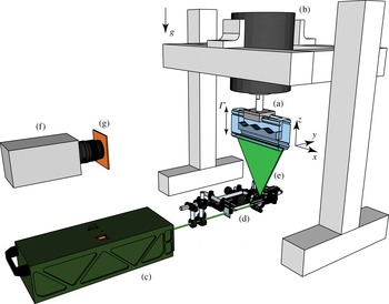
deep. An aluminium piece attached to the top couples the trough to an electromechanical shaker (Dynamic Systems VTS-80). A function waveform generator (Rigol DG-1022) and a bipolar amplifier (NF HSA-4011) generate a sinusoidal signal with tuneable amplitude and frequency which properly feeds the shaker. The acceleration of the system is precisely measured using an accelerometer (PCB Piezotronics 340A65) and a lock-in amplifier (Stanford Research SR830), synchronised with the shaker input signal. A second channel of the function waveform generator is used to create a synchronisation signal that triggers the imaging system at a programmable phase.
Experimental set-up. A Plexiglas trough (a) is vertically driven by an electromagnetic shaker (b). A double-pulsed laser (c) and an optical array (d) generate a light sheet (e) which passes through the trough. A high-speed camera (f) and a long-pass filter (g) acquire the images for PIV.

The upside-down configuration chosen for the experiment allows the system to be illuminated from the bottom, which is the only way to avoid undesired light refractions for the PIV imaging. A scheme of the set-up is displayed in figure 1. Further details can be found in Gordillo & Mujica (Reference Gordillo and Mujica2014). The PIV imaging system consists of a double-pulsed Nd:YAG laser (Quantel Evergreen 70) and a high-speed camera (Phantom v641), properly synchronised. The laser beam passes through an optical system which projects a
 $2~\text{mm}$
thick laser sheet into the trough. The optical system, mounted on a translational stage, allows the position of the illuminated plane to be freely adjusted in the
 $y$
direction.
In all of our runs, we fill the trough up to
 $h=20~\text{mm}$
with an aqueous solution of potassium bromide (KBr). The concentration,
 $13.7\,\%$
, is such that the density of the solution matches the density of the seeding particles (Kanomax Fluostar,
 $\varnothing =15~\unicode[STIX]{x03BC}\text{m}$
) i.e.
 $\unicode[STIX]{x1D70C}=1.1~\text{g}~\text{cm}^{-3}$
(cf. tables for aqueous solutions in Lide Reference Lide2004). The seeding particles are fluorescent, a feature that is used to create sharp images. A long-pass filter placed in front of the objective lens filters off any reflection of the laser sheet on the free surface, and only the light emitted by the fluorescent particles reaches the camera sensor. A small amount of wetting agent,
 $2~\text{ml}$
of Kodak Photoflo, is also added to the solution. The inclusion of this agent has been shown to improve wall wettability in this kind of system (Wu, Keolian & Rudnick Reference Wu, Keolian and Rudnick1984). Some ethyl alcohol (less than
 $1~\text{ml}$
) was used to previously dissolve the PIV seeding particles into water, avoiding the formation of clusters. The mixture of seeding particles was then kept in a syringe and added manually to the water until the concentration of particles in images was suitable for PIV (four particles in an
 $8\times 8$
pixel window, Raffel et al.
Reference Raffel, Willert, Wereley and Kompenhans2007).
Faraday waves are generated at the free surface of the fluid when the forcing acceleration
 $\unicode[STIX]{x1D6E4}$
is increased above a threshold
 $\unicode[STIX]{x1D6E4}_{0}$
, which is a function of the forcing frequency
 $2f$
. The waves are subharmonic, i.e. they oscillate at half of the forcing frequency
 $f$
. The wavelength
 $\unicode[STIX]{x1D706}$
and wavenumber
 $k=2\unicode[STIX]{x03C0}/\unicode[STIX]{x1D706}$
are related to the natural frequencies of the surface
 $f_{m,n}=\unicode[STIX]{x1D714}_{m,n}/(2\unicode[STIX]{x03C0})$
through the dispersion relation for closed basins,
 $$\begin{eqnarray}\unicode[STIX]{x1D714}_{m,n}^{2}=gk\tanh kh.\end{eqnarray}$$
The quantity
 $k$
is the modulus of the wavenumber
 $\boldsymbol{k}=(k_{x},k_{y})=(m\unicode[STIX]{x03C0}/L_{x},n\unicode[STIX]{x03C0}/L_{y})$
, and
 $m,n\in \mathbb{Z}$
are the numbers of nodes in each direction (for more details, cf. Miles Reference Miles1976). For a forcing frequency
 $2f$
close to
 $2f_{m,n}$
, the systems responds with a wavelength given by (2.1). The sign of the detuning
 $\unicode[STIX]{x0394}f=f-f_{m,n}$
defines whether the onset of the Faraday waves is subcritical (
 $\unicode[STIX]{x0394}f<0$
) or supercritical (
 $\unicode[STIX]{x0394}f>0$
), as shown by Douady (Reference Douady1990).
2.2 Observation of the streaming patterns
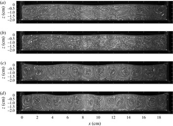
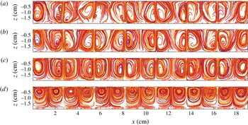
At first glance, the flow beneath the free surface is very simple: the fluid is carried from one crest to the neighbouring ones and then back through a cycle (Van Dyke Reference Van Dyke1982). However, particles do not come back exactly to the same position after each cycle. This fact can be easily observed when taking images stroboscopically. An overexposed image with strobe flashing shows the slow tracks followed by particles after several cycles (see figure 2). These tracks will be referred to as streaming patterns, and their study, as the streaming flow or velocity field related to it, is the main goal of this work.
Streaming patterns beneath purely longitudinal Faraday waves for (a)
 $2f=7.6~\text{Hz}$
, (b)
 $2f=8.9~\text{Hz}$
, (c)
 $2f=9.9~\text{Hz}$
and (d)
 $2f=10.8~\text{Hz}$
in the midplane in the crosswise direction (
 $y=L_{y}/2$
). The images were obtained by strobe illumination. The number of nodes of the standing Faraday wave is respectively
 $m=4,5,6,7$
(
 $n=0$
). The surface-wave amplitude
 $\unicode[STIX]{x1D701}$
for each case is respectively (a)
 $3.1~\text{mm}$
, (b)
 $1.9~\text{mm}$
, (c)
 $3.3~\text{mm}$
, (d)
 $3.4~\text{mm}$
.

Although the streaming patterns were observed indirectly by Faraday (Reference Faraday1831) through the accumulation of particles on the bottom of the trough, the first visualisation is due to Douady (Reference Douady1990), who used Kalliroscope particles for this purpose.
The streaming patterns are generated by a secondary flow which is very small compared with the main oscillatory flow. In our experiments, the streaming velocity field is typically around 20 times weaker than the oscillatory velocity field (Gordillo & Mujica Reference Gordillo and Mujica2014). Despite its weakness, the streaming patterns can be easily observed using a strobe light as a consequence of the fact that the main flow (the dominant velocity signal) is periodical whereas the streaming flow is mainly steady. Hence, the motion that particles undergo after a complete cycle due to the oscillatory field is zero, and only the contribution of the streaming velocity field is observed. It should be noted that particles under the free surface of a standing wave, which is the case of Faraday waves, have a Stokes drift (Stokes Reference Stokes1847) equal to zero after a complete cycle (Gordillo Reference Gordillo2012).
The streaming patterns also show a weak dependence on the phase at which the images are captured. Naturally, the patterns are distorted with the deformation of the free surface at a given phase. For the sake of simplicity, all of the quantitative measurements of the streaming field are performed at the phase at which the free surface is flat and only on longitudinal Faraday waves (no crosswise component, i.e.
 $n=0$
in (2.1)). For the same reason, all of the measurements shown here are restrained to the midplane in the
 $y$
direction.
The images in figure 2 also show that the structure of the streaming patterns is highly three-dimensional, even for Faraday waves with no crosswise component on the surface. Particles may enter and exit the illuminated plane, which explains the observed spiral trajectories followed by the particles.
2.3 Measurement protocol
To characterise the dependence of the streaming patterns on the amplitude and the frequency, we performed several experimental runs. The protocol was automatised using MATLAB, which controlled, via several interfaces (GPIB, USB, RS232 and Ethernet), all of the devices involved in the experiment. Each set of measurements analysed a single forcing frequency. The protocol was as follows. First, the amplitude was increased until stationary Faraday waves with large amplitude emerged. A downward-ramp scheme in amplitude was then followed. For each amplitude, we recorded a first series of 36 images, which completed a cycle, to determine the shape of the interface in terms of the phase (or time). Immediately afterwards, the shape of the free surface was detected using a standard algorithm for edge detection. After the flat-state phase was determined, the synchronisation signal was shifted and a second run consisting of 64 stroboscopic flat-state images was recorded. Measurements were made cyclically every four minutes, following the downward ramp until the Faraday waves on the surface vanished.
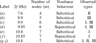
In table 1, we display a list of the experiments performed. In all cases, the wave at the surface was stationary and purely longitudinal. (The only slight deviation in the transverse direction is due to wetting between the fluid and the solid wall, which does not introduce a significant perturbation to the flow.) The runs include different frequencies and different wavenumbers. We also studied different nonlinear scenarios, i.e. subcritical and supercritical behaviour. Measurement ramps lasted between 1 and 4 h, depending on the initial amplitude and the ramp step size.
Set of measurements for the streaming patterns. Each line corresponds to a ramp in amplitude. The set includes four different wavelengths. Faraday waves destabilise through subcritical or supercritical bifurcations depending on the frequency detuning. Both subcritical and supercritical behaviours are explored. The last column shows the observed type of streaming pattern.

2.4 Experimental results
Our sequences of images were processed by means of two different techniques. In a very simple way, the sequences can be used to detect the trajectories followed by the seed particles. A synthetic overexposed image is obtained by maximising the grey value of each pixel along several frames. This is actually how the images in figure 2 were obtained. This strategy allows us to rapidly probe the streaming patterns and provides a powerful qualitative tool to analyse the data on the run. The second technique is PIV, which generates precise quantitative data. For this purpose, each sequence of images was analysed using our own PIV code. After preparing masks and background subtraction, we used time averaging in the correlation-function space to improve the signal-to-noise ratio (Meinhart, Wereley & Santiago Reference Meinhart, Wereley and Santiago2000). This allowed us to obtain neat velocity fields with a high spatial resolution (
 $8\times 8$
pixel window size, equivalent to
 $0.64\times 0.64~\text{mm}^{2}$
resolution) and no spatial averaging (0 % overlapping).
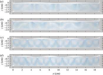
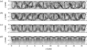
Velocity fields of the streaming patterns shown in figure 2 (increasing wavenumber from (a) to (d)). The background shows the shape of the interface
 $20\,\text{ms}$
after the flat phase. Panels (a,c,d) show ordered patterns with a spatial period equal to half of the surface waves. Panel (b) shows a distorted streaming pattern. The values for the wave amplitude
 $\unicode[STIX]{x1D701}$
are the same as in figure 2.

Figures 2 and 3 show respectively the streaming pattern and the velocity field
 $(u,w)$
in the
 $(x,z)$
-plane for four different forcing frequencies. The presented cases are a good representation of the whole set of collected data. In all of our measurements, we observe (i) a sequence of counter-rotating structures with a wavelength equal to half of the free-surface wavelength, (ii) that the velocity field strength decreases with depth and (iii) that the fluid is pushed downward at the free-surface antinodes and upward at the nodes. However, there are clear differences between the flow structures in the panels presented in figures 2 and 3. Based on our results and qualitative criteria, we identify three types of streaming pattern.
- Type I:
-
sequence of counter-rotating rolls (c and d).
- Type II:
-
sequence of moustache-shaped swirls (a).
- Type III:
-
irregular patterns (b).
Although only types I and II show ordered structures, type III displays well-shaped rolls next to the lateral walls at
 $x=0$
and
 $x=L_{x}$
. Types I and II share another common feature: both display squeezed counter-rotating structures at the bottom.
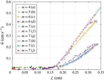
To illustrate quantitatively the classification described above, we chose two quantities that characterise the state of the system. The first one is the peak amplitude
 $\unicode[STIX]{x1D701}$
of the Faraday wave and is used to quantify the state of the free surface. This quantity can be obtained from the sequence of images used for determining the flat state (see § 2.3). As the second parameter, intended to represent the state of the flow, we chose the amplitude (along the
 $x$
coordinate) of the vertically averaged velocity
 $w$
, i.e.
 $$\begin{eqnarray}{\hat{w}}\equiv \max _{x\unicode[STIX]{x1D716}D}\left|\frac{1}{h}\int _{-h}^{0}\,\text{d}z\,w(x,y=L_{y}/2,z)\right|.\end{eqnarray}$$
Since the lateral walls induce strong coherent structures for all of the types, the domain
 $D$
is chosen such that the first and last rolls are removed, i.e.
 $D:[\unicode[STIX]{x1D706}/4,L_{x}-\unicode[STIX]{x1D706}/4]$
. The quantity
 ${\hat{w}}$
can be easily obtained from PIV data (the discretised
 $\text{d}z$
is
 $0.64~\text{mm}$
). Averaging along
 $z$
cancels noise induced by PIV detection.
Bifurcation diagram for streaming patterns. The diagram shows all of the collected data which collapse into two branches. The upper branch contains type-I streaming patterns (roll structures) and the lower one type-II swirl patterns. Type-III (filled symbols) irregular patterns can only be observed for very low amplitudes.

The two chosen quantities are plotted against each other in figure 4 for all of our measurements. For values of
 $\unicode[STIX]{x1D701}$
below some threshold
 $\unicode[STIX]{x1D701}_{c}\approx 1.5~\text{mm}$
,
 ${\hat{w}}$
remains almost equal to zero, which is related to the absence of periodic structures. Beyond this threshold,
 ${\hat{w}}$
bifurcates into two branches, each containing a large number of collapsed measurement points. All type-I (rolls) streaming patterns collapse to the upper branch, while type-II (swirls) patterns collapse to the lower one. The upper branch displays
 ${\hat{w}}$
values twice as strong as than the lower one. Type-III (irregular) patterns can be observed only for low
 ${\hat{w}}$
values, which gives a hint to understand their existence. A reasonable explanation is that the coherent periodic structures induced by the Faraday waves are so weak that they compete with weak parasitic large-scale eddies. The latter are presumably generated by surface tension effects and persist for long times, even after the vibration is switched off.
Figure 4 reveals that subcritical or supercritical behaviour does not have any relevant effect on streaming patterns: series (c,d) form a continuous line for
 $m=6$
; the same stands for series (e,f), where
 $m=7$
. More strikingly, type-I (rolls) and type-II (swirls) patterns may emerge regardless the value of
 $\unicode[STIX]{x1D706}$
. The evidence for
 $m=7$
is remarkable, because both types are observed with the same forcing parameters: type I, runs (e,f,h) and type II, runs (i,j). The mixture in the trough was the same and most of the runs were taken during the same day. We could not find a way to choose which streaming-flow pattern (I or II) was going to be selected during an experiment: the system spontaneously chooses one and keeps it until the wave on the surface vanishes. Multistability of viscous modes has been observed in other flows; e.g. Coles (Reference Coles1965) observed more than 20 different states in Taylor–Couette flow under the same forcing parameters.
As a closing for this section, we would like to readdress the effect of the streaming patterns at long time scales on particles in the liquid. Consider a particle subjected to the flow under Faraday waves. Besides the oscillating forces due to the rapidly oscillating velocity field, our particle is subjected to a viscous steady force due to the streaming flow. Hence, at long time scales, the particle will be slowly drifted by this force until it reaches a stagnation point. Particles heavier than the fluid will accumulate at stagnation points at the bottom of the trough, creating the heaps observed by Faraday in his seminal experiments. Particles lighter than the fluid will float at the free surface and accumulate into rafts, as has been shown in experiments by Falkovich et al. (Reference Falkovich, Weinberg, Denissenko and Lukaschuk2005) and Sanli et al. (Reference Sanli, Lohse and van der Meer2014). Streaming flows are thus a relevant extra ingredient to understand the motion induced on particles on Faraday waves. A step forward is to build a model able to predict the streaming patterns observed in our experiments. The next section is devoted to this task.
3 Theory
We consider a three-dimensional infinite layer of an incompressible and viscous fluid (density
 $\unicode[STIX]{x1D70C}$
and kinematic viscosity
 $\unicode[STIX]{x1D708}$
) bounded by flat impermeable walls and a top free surface. Locally, the flow far from the walls is tangent to them and periodic in time. Our goal is to determine the stationary component, or streaming, due to this periodic flow. As shown by the seminal work of Schlichting (Reference Schlichting1932) (see also Batchelor Reference Batchelor2000, pp. 353–364) in two-dimensional flows, streaming is the result of a complex mechanism that couples the flow inside the bulk (far from the walls) and at the boundary layers (near the walls). The coupling can be split into three intermediate mechanisms:
-
(i) the oscillatory flow in the bulk induces an oscillating boundary layer;
-
(ii) the oscillating boundary layer exerts a feedback on the bulk flow whose steady component originates the streaming;
-
(iii) the streaming is diffused into the bulk due to a viscous process.
The same mechanisms have been proved to be valid in three dimensions by Nicolás & Vega (Reference Nicolás and Vega2003), who also built a robust general approach that considers smoothly curved geometries.
In general, the viscous-streaming theory requires a twofold hypothesis: weak convection-to-inertia ratio and a wide length scale separation between the viscous boundary layer and the bulk flow. The two assumptions can be written in terms of the Strouhal number
 $St$
and the Reynolds number
 $Re$
:
 $St\equiv \unicode[STIX]{x1D706}/\unicode[STIX]{x1D701}\gg 1$
and
 $R\equiv Re\cdot St=(\unicode[STIX]{x1D706}/\unicode[STIX]{x1D6FF})^{2}\gg 1$
, where
 $\unicode[STIX]{x1D701}$
and
 $\unicode[STIX]{x1D706}$
are respectively the wave amplitude and wavelength. The length scale
 $\unicode[STIX]{x1D6FF}\equiv \sqrt{2\unicode[STIX]{x1D708}/\unicode[STIX]{x1D714}}$
and represents the extent of the viscous boundary layer.
The calculation of the three-dimensional viscous-streaming theory requires the application of boundary layer theory and multiscale analysis, leading to surprisingly compact final results. The effect of boundary layers can be finally written as boundary conditions for the streaming velocity field. Furthermore, the streaming-flow equations for the bulk remarkably resemble classical Navier–Stokes equations.
In §§ 3.1 and 3.2, we present briefly the results of Nicolás & Vega (Reference Nicolás and Vega2003) and other references. For the sake of simplicity, we focus on the standing-wave case, which is the relevant one for the analysed Faraday waves. The results provide the streaming boundary conditions for Faraday waves in § 3.3, which will be used to solve the streaming Navier–Stokes equations in § 4.
3.1 Viscous streaming due to oscillatory boundary layers
3.1.1 Streaming due to a fixed boundary
Due to the high shear in the vicinity of fixed boundaries, rigid walls emerge as the main source of streaming. In general, every wall of the container induces streaming (see figure 1 in Nicolás & Vega Reference Nicolás and Vega2003). For every fixed boundary, we denote a local coordinate system (
 $x,y,z$
) and define
 $u$
,
 $v$
and
 $w$
as the components of the velocity along the
 $x$
,
 $y$
and
 $z$
directions respectively. The local coordinates are chosen such that the
 $z$
axis is normal to the wall and points towards the bulk (
 $z=0$
at the wall). The
 $z$
domain is split into two subdomains: an inner region which comprises the boundary layer at the vicinity of the wall (
 $z\ll \unicode[STIX]{x1D6FF}$
) and an outer region extending beyond the boundary layer (
 $z\gg \unicode[STIX]{x1D6FF}$
). The fields inside the boundary layer are denoted
 $u$
,
 $v$
,
 $w$
and
 $p$
, standing for the components of the velocity and the pressure. The fields can be expanded as
 $q=\unicode[STIX]{x1D716}\sum _{i=0}^{\infty }\unicode[STIX]{x1D716}^{i}q_{i}$
, where
 $\unicode[STIX]{x1D716}\ll 1$
. Outside the boundary layer, the outer flow is denoted by the fields
 $\text{}\underline{u}$
,
 $\text{}\underline{v}$
,
 $\text{}\underline{w}$
and
 $\text{}\underline{p}$
. The outer flow is externally imposed, assumed to be periodical and of order
 $O(\unicode[STIX]{x1D716})$
, as
 $\unicode[STIX]{x1D6FF}\ll z\ll \unicode[STIX]{x1D706}$
, and is given by the general form
 $$\begin{eqnarray}\displaystyle (\text{}\underline{u},\text{}\underline{v},\text{}\underline{w})=\text{Re}\{(U_{0}(x,y,z),V_{0}(x,y,z),0)\text{e}^{\text{i}\unicode[STIX]{x1D714}t}\}. & & \displaystyle\end{eqnarray}$$
The length scales of variation in the three directions
 $x,y$
and
 $z$
are assumed to be of order
 $\unicode[STIX]{x1D706}$
, in agreement with the features of our experiments. As shown in detail in Nicolás & Vega (Reference Nicolás and Vega2003), it can be shown that if
 $St^{-1}=O(\unicode[STIX]{x1D716})$
and
 $Re^{-1}=O(\unicode[STIX]{x1D716})$
, the velocity field inside the boundary layer
 $(z\ll \unicode[STIX]{x1D6FF})$
at dominant order is given by
 $$\begin{eqnarray}\displaystyle \left.\begin{array}{@{}c@{}}\displaystyle u_{0}(x,y,z,t)=\text{Re}\{U_{0}(x,y,0)(1-\text{e}^{-\unicode[STIX]{x1D6FC}z/\unicode[STIX]{x1D6FF}})\text{e}^{\text{i}\unicode[STIX]{x1D714}t}\},\\ \displaystyle v_{0}(x,y,z,t)=\text{Re}\{V_{0}(x,y,0)(1-\text{e}^{-\unicode[STIX]{x1D6FC}z/\unicode[STIX]{x1D6FF}})\text{e}^{\text{i}\unicode[STIX]{x1D714}t}\},\\ \displaystyle w_{1}(x,y,z,t)=\text{Re}\left\{\unicode[STIX]{x1D6FF}(\unicode[STIX]{x2202}_{x}U_{0}+\unicode[STIX]{x2202}_{y}V_{0})|_{z=0}\left[\frac{1}{\unicode[STIX]{x1D6FC}}(1-\text{e}^{-\unicode[STIX]{x1D6FC}z/\unicode[STIX]{x1D6FF}})-\left(\frac{z}{\unicode[STIX]{x1D6FF}}\right)\right]\text{e}^{\text{i}\unicode[STIX]{x1D714}t}\right\},\end{array}\right\} & & \displaystyle\end{eqnarray}$$
where
 $\unicode[STIX]{x1D6FC}=(1+\text{i})$
and
 $w_{0}=0$
. In the case
 $U_{0}(x,y,z)=U_{0}$
,
 $V_{0}(x,y,z)=V_{0}$
and
 $W_{0}(x,y,z)=0$
, this solution reduces to the oscillatory boundary layer found by Stokes (Reference Stokes1851), which is an exact solution of the Navier–Stokes equation.
Likewise, it can be shown (cf. § 4 in Nicolás & Vega Reference Nicolás and Vega2003) that the interaction of the velocity field in (3.2) via the convective term in the Navier–Stokes equation leads to a steady streaming inside the boundary layer at
 $O(\unicode[STIX]{x1D716}^{2})$
. After imposing an asymptotic matching at
 $\unicode[STIX]{x1D6FF}\ll z\ll \unicode[STIX]{x1D706}$
, it follows that the streaming field is given by
 $$\begin{eqnarray}\displaystyle & \displaystyle \langle \text{}\underline{\boldsymbol{u}}_{\Vert }\rangle ^{z\rightarrow 0}=-\frac{1}{4\unicode[STIX]{x1D714}}\{\text{Re}[(\boldsymbol{U}_{0\Vert }^{\ast }\boldsymbol{\cdot }\unicode[STIX]{x1D735}_{\Vert })\boldsymbol{U}_{0\Vert }+2\boldsymbol{U}_{0\Vert }^{\ast }\unicode[STIX]{x1D735}_{\Vert }\boldsymbol{\cdot }\boldsymbol{U}_{0\Vert }]+3\text{Im}(\boldsymbol{U}_{0\Vert }^{\ast }\unicode[STIX]{x1D735}_{\Vert }\boldsymbol{\cdot }\boldsymbol{U}_{0\Vert })\}, & \displaystyle\end{eqnarray}$$
 $$\begin{eqnarray}\displaystyle & \displaystyle \langle \text{}\underline{w}\rangle ^{z\rightarrow 0}=0. & \displaystyle\end{eqnarray}$$
Here,
 $\boldsymbol{U}_{0\Vert }\equiv (U_{0},V_{0},0)$
,
 $_{\Vert }$
denotes projection on the plane parallel to the boundary and
 $^{\ast }$
the complex conjugate. Further simplifications can be made if the outer flow satisfies
 $\boldsymbol{U}_{0\Vert }=\boldsymbol{{\mathcal{U}}}_{0\Vert }(x,y)\text{e}^{\text{i}\unicode[STIX]{x1D6E9}(x,y)}$
, where the magnitude
 $\boldsymbol{{\mathcal{U}}}_{\mathbf{0}}$
is a real vector and the phase
 $\unicode[STIX]{x1D6E9}$
is a real scalar:
 $$\begin{eqnarray}\langle \text{}\underline{\boldsymbol{u}}_{\Vert }\rangle ^{z\rightarrow 0}=-\frac{1}{4\unicode[STIX]{x1D714}}[(\boldsymbol{{\mathcal{U}}}_{\mathbf{0}\Vert }\boldsymbol{\cdot }\unicode[STIX]{x1D735}_{\Vert })\boldsymbol{{\mathcal{U}}}_{\mathbf{0}\Vert }+2\,\boldsymbol{{\mathcal{U}}}_{\mathbf{0}\Vert }\unicode[STIX]{x1D735}_{\Vert }\boldsymbol{\cdot }\boldsymbol{{\mathcal{U}}}_{\mathbf{0}\Vert }+3\,\boldsymbol{{\mathcal{U}}}_{\mathbf{0}\Vert }(\boldsymbol{{\mathcal{U}}}_{\mathbf{0}\Vert }\boldsymbol{\cdot }\unicode[STIX]{x1D735}_{\Vert })\unicode[STIX]{x1D6E9}],\end{eqnarray}$$
which is consistent with the two-dimensional case (e.g. see Batchelor Reference Batchelor2000, equation (5.13.20)). The last term of this expression vanishes in the case of standing waves. Equation (3.5) is of utmost importance for our model because it highlights the source of the streaming and how it couples with the outer flow, i.e. the bulk. In practical terms, it can be regarded as the boundary condition for the streaming velocity field of the outer flow, as
 $z\rightarrow 0$
(more precisely, as
 $\unicode[STIX]{x1D6FF}\ll z\ll \unicode[STIX]{x1D706}$
).
3.1.2 Streaming due to a liquid–air interface
Calculations to determine an analogous formula to (3.5) for free surfaces pose a further challenge due to the coupling of the velocity field and the motion of the liquid–air interface. Let us denote the interface position as
 $z=\text{Re}\{\unicode[STIX]{x1D701}(x,y)\text{e}^{\text{i}\unicode[STIX]{x1D714}t}\}$
and assume that
 $\unicode[STIX]{x1D701}$
admits an expansion in terms of
 $\unicode[STIX]{x1D716}$
like that of the other fields. Herein, we analyse only two cases, which are linked to the degree of contamination on the interface.
-
(i) For a clean interface, Nicolás & Vega (Reference Nicolás and Vega2003, § 5) showed in detail that the matching conditions on the outer flow as we approach the free surface are
(3.6) $$\begin{eqnarray}\displaystyle & \displaystyle \unicode[STIX]{x2202}_{z}\langle \text{}\underline{\boldsymbol{u}_{\Vert }}\rangle ^{z\rightarrow 0}+\unicode[STIX]{x1D735}_{\Vert }\langle \text{}\underline{w}\rangle ^{z\rightarrow 0}=\text{Re}\{\unicode[STIX]{x1D735}_{\Vert }[\unicode[STIX]{x1D735}_{\Vert }\boldsymbol{\cdot }(\unicode[STIX]{x1D701}_{0}^{\ast }\boldsymbol{U}_{0})+(\unicode[STIX]{x1D735}_{\Vert }\unicode[STIX]{x1D701}_{0}^{\ast }\boldsymbol{\cdot }\unicode[STIX]{x1D735}_{\Vert })\boldsymbol{U}_{0}+(\unicode[STIX]{x1D735}_{\Vert }\boldsymbol{\cdot }\boldsymbol{U}_{0})\unicode[STIX]{x1D735}_{\Vert }\unicode[STIX]{x1D701}_{0}^{\ast }]\}, & \displaystyle \nonumber\\ \displaystyle & & \displaystyle\end{eqnarray}$$
(3.7)where we have assumed that the unperturbed free surface (with no vertical forcing) is flat for simplicity. These expressions considerably reduce in the case of standing waves as a consequence of
$$\begin{eqnarray}\displaystyle & \displaystyle \langle \text{}\underline{w}\rangle ^{z\rightarrow 0}={\textstyle \frac{1}{2}}\text{Re}[\unicode[STIX]{x1D735}_{\Vert }\boldsymbol{\cdot }(\unicode[STIX]{x1D701}_{0}^{\ast }\boldsymbol{U}_{0})], & \displaystyle\end{eqnarray}$$
$\unicode[STIX]{x1D701}\propto \text{i}\boldsymbol{U}_{0}$
, yielding (3.8)
$$\begin{eqnarray}\displaystyle & \displaystyle \unicode[STIX]{x2202}_{z}\langle \text{}\underline{\boldsymbol{u}_{\Vert }}\rangle ^{z\rightarrow 0}=0, & \displaystyle\end{eqnarray}$$
(3.9)The two conditions can be interpreted respectively as (1) a free tangential-stress condition and (2) vanishing normal velocity, both applicable to the streaming flow.
$$\begin{eqnarray}\displaystyle & \displaystyle \langle \text{}\underline{w}\rangle ^{z\rightarrow 0}=0. & \displaystyle\end{eqnarray}$$
-
(ii) For contaminated surfaces, a film formed by contaminants affects the dynamic properties of the interface dramatically. Miles (Reference Miles1967) particularly showed that the presence of the film affects the dissipation rate, an effect that has been confirmed in experiments by Henderson & Miles (Reference Henderson and Miles1994). In theory, the film has also been shown to affect streaming flows by enhancing drift instabilities in annular containers (Martin & Vega Reference Martin and Vega2005).


An interesting limit arises when the film is saturated with contaminants, thus forming an inextensible liquid–air interface. Combining the derivations of Nicolás & Vega (Reference Nicolás and Vega2003) and Martin & Vega (Reference Martin and Vega2005), the fully contaminated limit requires the following matching conditions for the outer flow:
 $$\begin{eqnarray}\displaystyle \langle \text{}\underline{\boldsymbol{u}}_{\Vert }\rangle ^{_{z\rightarrow 0}} & = & \displaystyle -\frac{1}{4\unicode[STIX]{x1D714}}\{\!\text{Re}[(\boldsymbol{U}_{0\Vert }^{\ast }\boldsymbol{\cdot }\unicode[STIX]{x1D735}_{\Vert })\boldsymbol{U}_{0\Vert }+2\boldsymbol{U}_{0\Vert }^{\ast }\unicode[STIX]{x1D735}_{\Vert }\boldsymbol{\cdot }\boldsymbol{U}_{0\Vert }]\nonumber\\ \displaystyle & & \displaystyle +\,\text{Im}(3\boldsymbol{U}_{0\Vert }^{\ast }\unicode[STIX]{x1D735}_{\Vert }\boldsymbol{\cdot }\boldsymbol{U}_{0\Vert }-2\unicode[STIX]{x1D701}_{0}^{\ast }\unicode[STIX]{x1D735}_{\Vert }\unicode[STIX]{x1D701}_{0})\!\},\end{eqnarray}$$
 $$\begin{eqnarray}\displaystyle \langle \text{}\underline{w}\rangle ^{_{z\rightarrow 0}}=0 & & \displaystyle\end{eqnarray}$$
which for standing waves simplify to:
 $$\begin{eqnarray}\displaystyle & \displaystyle \langle \text{}\underline{\boldsymbol{u}}_{\Vert }\rangle ^{z\rightarrow 0}=-\frac{1}{4\unicode[STIX]{x1D714}}\{\text{Re}[(\boldsymbol{U}_{0\Vert }^{\ast }\boldsymbol{\cdot }\unicode[STIX]{x1D735}_{\Vert })\boldsymbol{U}_{0\Vert }+2\boldsymbol{U}_{0\Vert }^{\ast }\unicode[STIX]{x1D735}_{\Vert }\boldsymbol{\cdot }\boldsymbol{U}_{0\Vert }]\}, & \displaystyle\end{eqnarray}$$
 $$\begin{eqnarray}\displaystyle & \displaystyle \langle \text{}\underline{w}\rangle ^{z\rightarrow 0}=0. & \displaystyle\end{eqnarray}$$
The results are equal to those obtained for rigid boundaries (as a reference, in the notation of Martin & Vega (Reference Martin and Vega2005), the fully contaminated limit arises when
 $\unicode[STIX]{x1D6E4}\rightarrow 1$
(e.g.
 $d=-1$
and
 $a=-k/\unicode[STIX]{x1D714}_{0}$
in (A8) of this reference)).
3.2 Streaming in the bulk
The final step is to determine how the streaming due to the boundary layers induces a streaming in the bulk. For this purpose, consider the general Navier–Stokes equation for the bulk in a comoving frame of reference,
 $$\begin{eqnarray}\unicode[STIX]{x2202}_{t}\text{}\underline{\boldsymbol{u}}+(\text{}\underline{\boldsymbol{u}}\boldsymbol{\cdot }\unicode[STIX]{x1D735})\text{}\underline{\boldsymbol{u}}=-\frac{1}{\unicode[STIX]{x1D70C}}\unicode[STIX]{x1D735}\text{}\underline{p}+a(t)\hat{\boldsymbol{k}}+\unicode[STIX]{x1D708}\unicode[STIX]{x1D6FB}^{2}\text{}\underline{\boldsymbol{u}},\end{eqnarray}$$
where
 $a(t)=-g+\unicode[STIX]{x1D6E4}\cos 2\unicode[STIX]{x1D714}t$
is the vertical acceleration of the system. To simplify the notation, we omit the underline. We decompose the velocity and pressure field into oscillatory and steady terms,
 $\boldsymbol{u}(\boldsymbol{x},t)=\widetilde{\boldsymbol{u}}(\boldsymbol{x},t)+\overline{\boldsymbol{u}}(\boldsymbol{x})$
and
 $p(\boldsymbol{x},t)=\widetilde{p}(\boldsymbol{x},t)+\overline{p}(\boldsymbol{x})$
. For most Faraday-wave experiments, since
 $\unicode[STIX]{x1D706},h,L_{x},L_{y}\gg \unicode[STIX]{x1D6FF}$
, the flow under the waves is potential. Thus, if at dominant order
 $\widetilde{\boldsymbol{u}}$
scales as some small parameter
 $\unicode[STIX]{x1D716}\ll 1$
, the oscillatory vorticity will be a correction of higher order. Likewise, we expect that
 $\overline{\boldsymbol{u}}=O(\unicode[STIX]{x1D716}^{2})$
. To proceed, we write the convective term in (3.14) in terms of
 $\unicode[STIX]{x1D74E}$
,
 $(\boldsymbol{u}\boldsymbol{\cdot }\unicode[STIX]{x1D735})\boldsymbol{u}=\unicode[STIX]{x1D735}((1/2)\boldsymbol{u}^{2})-\boldsymbol{u}\times \unicode[STIX]{x1D74E}$
. By applying curl to (3.14), and selecting oscillatory terms, we obtain an equation for the oscillatory vorticity,
 $$\begin{eqnarray}\unicode[STIX]{x2202}_{t}\widetilde{\unicode[STIX]{x1D74E}}-\unicode[STIX]{x1D735}\times (\widetilde{\boldsymbol{u}}\times \overline{\unicode[STIX]{x1D74E}})+\text{h.o.t.}=0,\end{eqnarray}$$
which shows that
 $\widetilde{\unicode[STIX]{x1D74E}}=O(\unicode[STIX]{x1D716}^{3})$
at leading order. On the other hand, time averaging of (3.14) leads to
 $$\begin{eqnarray}\displaystyle \unicode[STIX]{x2202}_{t}\overline{\boldsymbol{u}}-\langle \widetilde{\boldsymbol{u}}\times \widetilde{\unicode[STIX]{x1D74E}}\rangle -\overline{\boldsymbol{u}}\times \overline{\unicode[STIX]{x1D74E}}=-\frac{1}{\unicode[STIX]{x1D70C}}\unicode[STIX]{x1D735}\left(\overline{p}+\unicode[STIX]{x1D70C}gz+\frac{1}{2}\unicode[STIX]{x1D70C}\langle \widetilde{\boldsymbol{u}}^{2}\rangle +\frac{1}{2}\unicode[STIX]{x1D70C}\langle \overline{\boldsymbol{u}}^{2}\rangle \right)+\unicode[STIX]{x1D708}\unicode[STIX]{x1D6FB}^{2}\overline{\boldsymbol{u}}, & & \displaystyle\end{eqnarray}$$
where we have kept the term
 $\unicode[STIX]{x2202}_{t}\overline{\boldsymbol{u}}$
to account for a weak slow time dependence of the steady flow. It should be noted now that for standing waves,
 $$\begin{eqnarray}\displaystyle \langle \widetilde{\boldsymbol{u}}\times \widetilde{\unicode[STIX]{x1D74E}}\rangle =\left\langle \widetilde{\boldsymbol{u}}\times \int \unicode[STIX]{x1D735}\times (\widetilde{\boldsymbol{u}}\times \overline{\unicode[STIX]{x1D74E}})\,\text{d}t\right\rangle =0, & & \displaystyle\end{eqnarray}$$
up to order
 $O(\unicode[STIX]{x1D716}^{4})$
, since the temporal part of the integral does not yield steady terms. (In non-standing waves, the latter expression yields extra terms such as a Stokes drift, as shown in full detail by Nicolás & Vega (Reference Nicolás and Vega2003).) Hence, we obtain for the streaming field in the bulk
 $$\begin{eqnarray}(\overline{\boldsymbol{u}}\boldsymbol{\cdot }\unicode[STIX]{x1D735})\overline{\boldsymbol{u}}=-\frac{1}{\unicode[STIX]{x1D70C}}\unicode[STIX]{x1D735}\left(\overline{p}+\unicode[STIX]{x1D70C}gz+\frac{1}{2}\unicode[STIX]{x1D70C}\langle \tilde{\boldsymbol{u}}^{2}\rangle \right)+\unicode[STIX]{x1D708}\unicode[STIX]{x1D6FB}^{2}\overline{\boldsymbol{u}}.\end{eqnarray}$$
By defining
 $\overline{p}^{\prime }\equiv \overline{p}+\unicode[STIX]{x1D70C}gz+(1/2)\unicode[STIX]{x1D70C}\langle \tilde{\boldsymbol{u}}^{2}\rangle$
, the equation for the steady part of
 $\boldsymbol{u}$
becomes identical to a Navier–Stokes equation for a steady flow with no external forcing. The equation is equivalent to the one derived by Nicolás & Vega (Reference Nicolás and Vega2003) in the particular case of non-propagating waves. On the other hand, it can be easily shown that the incompressibility condition for the steady field is the usual one,
 $$\begin{eqnarray}\unicode[STIX]{x1D735}\boldsymbol{\cdot }\overline{\boldsymbol{u}}=0.\end{eqnarray}$$
Equations (3.18) and (3.19) plus the boundary conditions found in §§ 3.1.1 and 3.1.2 contain all of the information required to determine the steady streaming in the bulk. Remarkably, the contribution due to the local oscillatory velocity field only appears in the effective pressure in (3.20) and has null effect on
 $\overline{\boldsymbol{u}}$
at leading order. The steady component of the flow stemming from the nonlinearities in the bulk is thus negligible in comparison with the streaming generated by the boundary layer. Henceforth, we expect that the boundary layers are mainly responsible for the appearance of streaming in quasi-inviscid stationary waves.
However, the framework we have presented still lacks an explanation to describe how the streaming flow evolves in time. For instance, the streaming field has non-vanishing vorticity: where does this vorticity come from? Batchelor (Reference Batchelor2000, see § 5.13, p. 361) gave an answer to this question: the steady streaming is only the final stage of a transient process, where vorticity is slowly transferred from the boundary layers into the volume. Considering that the transient process is much slower than any oscillating dynamics (e.g. the wave period or the transient to establish the surface wave), we can modify (3.18) to account for a slow temporal dependence of the streaming flow. The result is strikingly familiar,
 $$\begin{eqnarray}\unicode[STIX]{x2202}_{t}\overline{\boldsymbol{u}}+(\overline{\boldsymbol{u}}\boldsymbol{\cdot }\unicode[STIX]{x1D735})\overline{\boldsymbol{u}}=-\frac{1}{\unicode[STIX]{x1D70C}}\unicode[STIX]{x1D735}\overline{p}^{\prime }+\unicode[STIX]{x1D708}\unicode[STIX]{x1D6FB}^{2}\overline{\boldsymbol{u}},\end{eqnarray}$$
which is analogous to a full Navier–Stokes equation. On the other hand, the incompressibility condition naturally remains unchanged during the transient process.
So far, we have shown that the evolution equation for the streaming velocity field for non-propagating waves can be solved at dominant order by using full Navier–Stokes equations for the steady fields (an apparently naïve choice, but not so). Although there is a modified pressure and different boundary conditions, their application remains stunningly simple.
As a final comment, equation (3.20) stands for the average Eulerian velocity. For standing waves, both the Eulerian and the Lagrangian velocity are equal in the bulk (see Batchelor Reference Batchelor2000, pp. 353–364). However, the same is not valid inside the boundary layers, as shown by (3.2) (cf. Longuet-Higgins Reference Longuet-Higgins1953, figure 5), which leads to the inversion of the streaming direction. A remarkable example of streaming inversion has been reported in air-driven Chladni patterns in van Gerner et al. (Reference van Gerner, van der Weele, van der Hoef and van der Meer2011).
3.3 Classical Faraday waves
3.3.1 General case
Here, we apply the previous results to classical Faraday waves. The container is assumed to be a rectangular impermeable tank of horizontal dimensions
 $L_{x}$
,
 $L_{y}$
filled up to height
 $h$
. The fluid then occupies the domain
 $(x,y,z)\in [0,L_{x}]\times [0,L_{y}]\times [-h,0]$
.
In the limit of ideal flows, the oscillatory velocity field in Faraday waves at leading order is modelled by a well-known velocity potential
 $\unicode[STIX]{x1D6F7}$
inside the bulk,
 $$\begin{eqnarray}\unicode[STIX]{x1D6F7}(x,y,z,t)=A\cos (k_{x}x)\cos (k_{y}y)\frac{\cosh (k(z+h))}{\cosh (kh)}\cos (\unicode[STIX]{x1D714}t),\end{eqnarray}$$
where
 $k_{x}$
and
 $k_{y}$
are multiples of
 $\unicode[STIX]{x03C0}/L_{x}$
and
 $\unicode[STIX]{x03C0}/L_{y}$
respectively, and
 $k=\sqrt{k_{x}^{2}+k_{y}^{2}}$
. Here,
 $\boldsymbol{U}_{0}$
is related to
 $\unicode[STIX]{x1D6F7}$
through
 $\boldsymbol{U}_{0}=\unicode[STIX]{x1D735}\unicode[STIX]{x1D6F7}.$
Hence, the oscillatory tangential velocity field at the boundaries can be evaluated via (3.21) and then plugged into (3.5) to obtain the matched boundary condition for the outer streaming field. These streaming boundary conditions will then be used in § 4 to compute the streaming in the bulk through (3.20).
Vertical walls
At
 $x=\{0,L_{x}\}$
, the tangential velocity field is
 $$\begin{eqnarray}\displaystyle & \displaystyle \text{}\underline{u}_{0}=0, & \displaystyle\end{eqnarray}$$
 $$\begin{eqnarray}\displaystyle & \displaystyle (\text{}\underline{v}_{0},\text{}\underline{w}_{0})=\pm A\cos (\unicode[STIX]{x1D714}t)\left(-k_{y}\sin (k_{y}y)\frac{\cosh k(z+h)}{\cosh kh},k\cos (k_{y}y)\frac{\sinh k(z+h)}{\cosh kh}\right)\!\qquad & \displaystyle\end{eqnarray}$$
(the value of
 $\pm$
at
 $x=L_{x}$
is given by
 $\exp (\text{i}\unicode[STIX]{x03C0}L_{x})$
). Equation (3.23) is used to get the matched streaming boundary conditions by applying (3.5),
 $$\begin{eqnarray}\displaystyle & \displaystyle \langle \text{}\underline{u}_{1}\rangle =0, & \displaystyle\end{eqnarray}$$
 $$\begin{eqnarray}\displaystyle & \displaystyle (\langle \text{}\underline{v}_{1}\rangle ,\langle \text{}\underline{w}_{1}\rangle )=\frac{A^{2}}{8\unicode[STIX]{x1D714}C_{0}^{2}}(k_{y}\sin (2k_{y}y)[3k_{x}^{2}C_{z}^{2}-k^{2}],-kS_{2z}[3k_{x}^{2}\cos ^{2}(k_{y}y)+k_{y}^{2}]). & \displaystyle\end{eqnarray}$$
Here, we have compacted the notations
 $\cosh (k(z+h))$
,
 $\sinh (k(z+h))$
and
 $\sinh (2k(z+h))$
into
 $C_{z}$
,
 $S_{z}$
and
 $S_{2z}$
, respectively (
 $C_{0}$
stands for
 $\cosh (kh)$
). By permuting the coordinates
 $x\leftrightarrow y$
, components
 $u\leftrightarrow v$
and indices
 $_{x}\leftrightarrow \,_{y}$
, we deduce the matched streaming boundary conditions at the other two walls
 $y=\{0,L_{y}\}$
,
 $$\begin{eqnarray}\displaystyle & \displaystyle (\langle \text{}\underline{u}_{1}\rangle ,\langle \text{}\underline{w}_{1}\rangle )=\frac{A^{2}}{8\unicode[STIX]{x1D714}C_{0}^{2}}(k_{x}\sin (2k_{x}x)[3k_{y}^{2}C_{z}^{2}-k^{2}],-kS_{2z}[3k_{y}^{2}\cos ^{2}(k_{x}x)+k_{x}^{2}]), & \displaystyle\end{eqnarray}$$
 $$\begin{eqnarray}\displaystyle & \displaystyle \langle \text{}\underline{v}_{1}\rangle =0. & \displaystyle\end{eqnarray}$$
Bottom
At the tank bottom
 $(z=-h)$
, the instantaneous velocity reads
 $$\begin{eqnarray}(\text{}\underline{u}_{0},\text{}\underline{v}_{0})=-A\cos (\unicode[STIX]{x1D714}t)\left(k_{x}\frac{\sin (k_{x}x)\cos (k_{y}y)}{\cosh kh},k_{y}\frac{\cos (k_{x}x)\sin (k_{y}y)}{\cosh kh}\right)\end{eqnarray}$$
and the resulting matched boundary conditions are
 $$\begin{eqnarray}\displaystyle & & \displaystyle (\langle \text{}\underline{u}_{1}\rangle ,\langle \text{}\underline{v}_{1}\rangle )\nonumber\\ \displaystyle & & \displaystyle \quad =-\frac{A^{2}}{8\unicode[STIX]{x1D714}C_{0}^{2}}(k_{x}\sin (2k_{x}x)[3k^{2}\cos ^{2}(k_{y}y)-k_{y}^{2}],k_{y}\sin (2k_{y}y)[3k^{2}\cos ^{2}(k_{x}x)-k_{x}^{2}]),\qquad \quad\end{eqnarray}$$
 $$\begin{eqnarray}\langle \text{}\underline{w}_{1}\rangle =0.\end{eqnarray}$$
Top interface
At the interface (
 $z=0$
), we apply the two types of boundary conditions for the streaming field found in § 3.1.2. The first one is for the clean case,
 $$\begin{eqnarray}\displaystyle \left.\begin{array}{@{}c@{}}\displaystyle \unicode[STIX]{x2202}_{z}\langle \text{}\underline{u}_{1}\rangle =\unicode[STIX]{x2202}_{z}\langle \text{}\underline{v}_{1}\rangle =0,\\ \displaystyle \langle \text{}\underline{w}_{1}\rangle =0,\end{array}\right\} & & \displaystyle\end{eqnarray}$$
which is equivalent to the classic free-surface condition, i.e. null tangential stress at
 $z=0$
(Batchelor Reference Batchelor2000). The second one is
 $$\begin{eqnarray}\displaystyle \left.\begin{array}{@{}c@{}}\displaystyle \langle \text{}\underline{w}_{1}\rangle =0,\\ \displaystyle (\langle \text{}\underline{u}_{1}\rangle ,\langle \text{}\underline{v}_{1}\rangle )=-\frac{A^{2}}{8\unicode[STIX]{x1D714}} (\!k_{x}\sin (2k_{x}x)[3k^{2}\cos ^{2}(k_{y}y)-k_{y}^{2}],\\ \hspace{40.00006pt}k_{y}\sin (2k_{y}y)[3k^{2}\cos ^{2}(k_{x}x)-k_{x}^{2}]\!),\end{array}\right\} & & \displaystyle\end{eqnarray}$$
for a fully contaminated surface (similar to the streaming on a rigid boundary as stated in § 3.1.2).
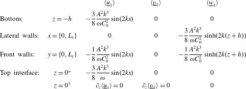
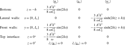
Streaming matched boundary conditions for longitudinal Faraday waves (
 $k=k_{x},\,k_{y}=0$
). Only the conditions at the top interface change for a fully contaminated interface (
 $^{\ast }$
) and a clean one (
 $^{\dagger }$
). These boundary conditions were used in the numerical simulations in § 4.
3.3.2 Case of longitudinal waves:
$k_{y}=0$

We now focus on the case of plane stationary waves characterised by
 $k_{y}=0$
, which corresponds to the striped Faraday-wave patterns that can easily be observed in containers whose transverse dimension is much smaller than the critical wavelength. Waves in this case are almost two-dimensional. Nevertheless, some three-dimensional effects may still be present due to the presence of the walls in the transverse direction, which induces alteration of the streaming flow through its viscosity. The expression for the instantaneous potential
 $\unicode[STIX]{x1D6F7}$
is thus changed to
 $$\begin{eqnarray}\unicode[STIX]{x1D6F7}(x,y,z,t)=A\cos (kx)\frac{\cosh k(z+h)}{\cosh kh}\cos (\unicode[STIX]{x1D714}t),\end{eqnarray}$$
where naturally
 $k_{x}=k$
. As a result, the matched boundary conditions for the streaming velocities are also simplified. The results are summarised in table 2.
3.3.3 Two-dimensional flow
When the problem is completely homogeneous in the
 $y$
direction (absence of transverse walls, implying
 $\unicode[STIX]{x2202}_{y}=0$
,
 $v=\langle \text{}\underline{v}_{1}\rangle =0$
), the potential takes the same expression as in the case
 $k_{y}=0$
(equation (3.33)). The matched boundary conditions in table 2 remain similar while those at the transverse walls drop. The transverse walls are the only source of differences between the
 $k_{y}=0$
and the two-dimensional flow. In the former case, the presence of the wall is expected to induce a three-dimensional streaming field.
4 Numerical simulations
In order to solve (3.20) with the matched boundary conditions from table 2 provided by the theory, we require numerical simulations. They allow us to address two basic questions. Can we reproduce experimental observations using the boundary-layer-induced streaming theory? Is it sufficient to keep a two-dimensional approximation, or do three-dimensional effects play an important role?
4.1 Numerical methods
To run simulations of the streaming flow inside the incompressible vibrating fluid, we implemented our own code. The code directly integrates the Navier–Stokes equations with the divergence-free condition (3.20) in a parallelepiped domain delimited at the top by the interface of the fluid at rest. The flat top interface is a fair approximation for the time-averaged position of low-amplitude Faraday waves. In (3.20), the gravity and the vertical vibration are gathered with the pressure to form a time-dependent effective pressure and do not have any effect on the velocity fields since a single fluid of constant density is involved in this model. In the code, the fields are discretised by finite-difference schemes using the MAC (marker and cell) disposition on a regular staggered mesh. The pressure is computed at the centre of each cell and the components of the velocity are located at the faces corresponding to their direction. The incompressible Navier–Stokes equations are solved by a projection method (Chorin Reference Chorin1968) and the pressure is computed incrementally with a BiCGStab (stabilised biconjugate gradient) method. The spatial discretisation is made with standard centred schemes of second order except for the advection terms, for which ENO (essentially non-oscillatory) schemes are used. The temporal stepping involves a first-order forward Euler discretisation with adaptive time steps to ensure numerical stability.
The simulations use the equations from table 2 as matched boundary conditions, with the three quantities
 $k$
,
 $\unicode[STIX]{x1D714}$
and
 $A$
fixed. We recall that for longitudinal waves, the wavenumber is defined as
 $k=m\unicode[STIX]{x03C0}/L_{x}$
, with
 $m$
an integer, and
 $\unicode[STIX]{x1D714}$
is deduced from
 $k$
by means of (2.1) in consistency with the experimental observations. We use as control parameter the velocity-potential amplitude
 $A$
(see (3.21)), which is related to the amplitude of Faraday waves via
 $$\begin{eqnarray}A\sim \frac{g\unicode[STIX]{x1D701}}{\unicode[STIX]{x1D714}},\end{eqnarray}$$
obtained by using the trivial dynamic boundary condition at the surface. Therefore, using (4.1) and the definitions for the Strouhal and Reynolds numbers from § 3, we can write the Reynolds number as
 $Re\equiv \unicode[STIX]{x1D706}\unicode[STIX]{x1D714}\unicode[STIX]{x1D701}/2\unicode[STIX]{x1D708}=\unicode[STIX]{x1D706}\unicode[STIX]{x1D714}^{2}A/2g\unicode[STIX]{x1D708}$
and the wave steepness as
 $St^{-1}\equiv \unicode[STIX]{x1D701}/\unicode[STIX]{x1D706}=\unicode[STIX]{x1D714}A/g\unicode[STIX]{x1D706}$
. We emphasise some features about the theoretical model and the simulations. First, the fact that the coefficients
 $k$
,
 $\unicode[STIX]{x1D714}$
and
 $A$
are set up manually renders the model and the simulations independent of the bifurcation criticality, a feature consistent with the experimental results. Second, all of the matched boundary conditions for the streaming flow are proportional to
 $A^{2}/\unicode[STIX]{x1D714}$
. Hence, cases with altered
 $\unicode[STIX]{x1D714}$
are also swept by varying
 $A$
; the complete model could be rewritten as a function of the single variable
 $A^{\prime }=A/\sqrt{\unicode[STIX]{x1D714}}$
instead of
 $\unicode[STIX]{x1D714}$
and
 $A$
separately, reducing the dimensions of the parameter space.
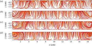
Streamlines in the
 $y$
midplane for
 $m=7$
with a clean liquid–air interface. The amplitude
 $A$
decreases from (a) to (d): (a)
 $35.5$
, (b)
 $20$
, (c)
 $11.3$
and (d)
 $0.2~\text{cm}^{2}~\text{s}^{-1}$
. Accordingly, the dimensionless parameters
 $(Re,St^{-1})$
for each case are (a)
 $12250,0.222$
, (b)
 $6890,0.125$
, (c)
 $3880,0.07$
and (d)
 $69,0.001$
.

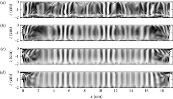
Streaming velocity field in the
 $y$
midplane for
 $m=7$
and varying
 $A$
. The interface is assumed to be clean. Amplitudes (as well as dimensionless parameters) are the same as in figure 5.

Streamlines in the
 $y$
midplane for
 $m=7$
and varying
 $A$
. The interface is fully contaminated. Amplitudes and dimensionless parameters are the same as in figure 5.

Streaming velocity field in the
 $y$
midplane for
 $m=7$
and varying
 $A$
. The interface is fully contaminated. Amplitudes and dimensionless parameters are the same as in figure 5.

4.2 Numerical results
In all of our simulations, we set the liquid properties and geometric parameters to match those in the experiment: the density
 $\unicode[STIX]{x1D70C}=1.1~\text{g}~\text{cm}^{-3}$
, the dynamic viscosity
 $\unicode[STIX]{x1D708}=9.09\times 10^{-3}~\text{cm}^{2}~\text{s}^{-1}$
, the dimensions of the fluid layer
 $L_{x}\times L_{y}\times h=(19.05\times 2.54\times 2)~\text{cm}^{3}$
and the number of nodes in the longitudinal direction
 $m=4,5,6,7$
. The corresponding frequencies of Faraday waves given by the dispersion relation (2.1) are
 $f=3.8$
Hz, 4.45 Hz, 4.95 Hz and 5.4 Hz respectively (the frequency of vibration of the container corresponds to
 $2f$
, as shown in table 1). The velocity-potential amplitude
 $A$
is varied between
 $0.2~\text{cm}^{2}~\text{s}^{-1}$
and
 $63~\text{cm}^{2}~\text{s}^{-1}$
, where the lowest bound is the value below which the streaming flow remains qualitatively unchanged and the upper bound is the value at which the code outcomes diverge. With these amplitudes, the Reynolds number ranges from
 $60$
to
 $2\times 10^{4}$
, and the steepness goes from
 $5\times 10^{-4}$
to
 $0.4$
(for specific values, see the caption to figure 5). All of our values largely meet the theoretical requirements of § 3, i.e. large
 $Re$
and small wave steepness
 $St^{-1}$
. In our simulations, we used a regular discretised mesh that contained
 $240\times 80\times 80$
cells. Simulations were performed with both clean and fully contaminated boundary conditions at the interface, cf. table 2.
In figures 5 and 6, we first show the streamlines and the associated streaming velocity field in the
 $y$
midplane. We specifically set
 $m=7$
,
 $f=5.4$
Hz on a clean interface as
 $A$
is varied. Likewise, in figures 7 and 8, we plot respectively the streamlines and the associated streaming velocity fields for the same values of
 $m$
and
 $\unicode[STIX]{x1D714},$
but for a fully contaminated liquid–air interface.
Comparison of figures 5 and 6 with 7 and 8 shows that contamination induces very unlike streaming flows at low amplitudes. The low-amplitude fully contaminated Faraday streaming flows are very similar to the type-I patterns (rolls) found in the experiments, with weak spiralling loops at the top of the domain and small recirculations at the bottom. The fact that the streaming flows do not form perfectly closed loops is related to the presence of transverse variations of the velocity component
 $v$
. The features of the flow are then expected to differ from those obtained with the two-dimensional theory, even on the
 $y$
midplane. The experimental patterns of type I (figures 2 and 3, patterns (c) and (d)) display the strongest similarities with the simulated fields of figures 7 and 8 at moderate amplitude
 $A=11.3~\text{cm}^{2}~\text{s}^{-1}$
. Therein, both the streamlines and the velocity fields have very similar shapes.
The clean-interface Faraday streaming flows look completely different from the fully contaminated ones and contrast with all of the patterns observed in the experiments. However, they display similarities to the type-II patterns (swirls), namely the presence of accumulation points in the vicinity of the interface, suggesting again that the flow is fairly three-dimensional on the
 $y$
midplane. In contrast, there are no loops at the top of the domain. Intermediate degrees of contamination on the interface, which yield matched boundary conditions between (3.31) and (3.32), have been introduced by Martin et al. (Reference Martin, Martel and Vega2002) for 2D flows and might improve the resemblance between experiments and simulations.
When the amplitude goes beyond
 $A\approx 25~\text{cm}^{2}~\text{s}^{-1}$
, ordered streaming structures destabilise, giving rise to unsteady patterns (see panel (a) in figures 5–8). The patterns oscillate on time scales that are still much slower than the oscillation period, in agreement with the hypotheses of § 3.2. Although a full description of the onset of this instability is out of the scope of this work, we point out that these dynamical regimes appear regardless of the interface contamination and for all of the wavenumbers that we explored.
On the other hand, varying the wavenumber
 $m$
in the boundary conditions does not have any dramatic effect on the flow structure. Besides the expected change of wavelength of the streaming flows that occurs, the loops at the walls are overcome by the central patterns as
 $m$
is decreased, particularly in the clean case.
To see whether the two-dimensional approximation used in previous works is good enough to explain the streaming field qualitatively, we exploit the three-dimensional data obtained from the numerical simulations. First, we compare the three-dimensional streaming patterns of our numerical simulations in the
 $y$
midplane (figures 5–8) with their two-dimensional counterparts (figure 9) at low amplitude,
 $A=0.2~\text{cm}^{2}~\text{s}^{-1}$
, and for
 $m=7$
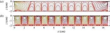
. For this purpose, we ran a two-dimensional simplified version of the code following § 3.3.3. The main qualitative differences between the streaming fields of figures 5–8 and the two-dimensional ones of figure 9 stem from the fact that streamlines become perfectly closed loops when the flow is purely two-dimensional, as expected. The differences are localised near the walls of the domain and are especially striking in the clean case (compare figure 9
a with figures 5
d and 6
d). The differences remain visible when the interface is contaminated at the frontier between two superposed loops, but to a lesser extent (compare figure 9
b with figures 7
d and 8
d). Nevertheless, the main differences between the two-dimensional streaming flows and the three-dimensional ones are located in regions where the streaming velocity is weak.
Velocity fields (arrows) and streamlines (contours) of the two-dimensional streaming flow for
 $m=7$
and
 $A=0.2~\text{cm}^{2}~\text{s}^{-1}$
; (a) clean and (b) fully contaminated interface.

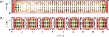
Velocities of the streaming flow in the horizontal plane
 $z=-1$
cm for
 $m=7$
and
 $A=0.2~\text{cm}^{2}~\text{s}^{-1}$
. Arrows represent the horizontal velocity components (
 $u,v$
) while contours represent
 $w$
; (a) clean and (b) fully contaminated interface.

In our three-dimensional simulations, the transverse effects are more visible in horizontal planes, for instance at
 $z=-1~\text{cm}$
, as shown in figure 10. They are highlighted by significant gradients of
 $w$
in the transverse direction. Likewise, perceptible deviations of the velocity from or towards the midplane
 $y=L_{y}/2$
are observed. The transverse effects are more marked near the walls and are exacerbated with increasing wave amplitude
 $A$
and decreasing trough width
 $L_{y}$
.
Further insights about three-dimensional effects can be gained by tracking small fluid parcels inside the bulk. For the sake of simplicity, we restrict ourselves to the lowest-amplitude patterns,
 $A=0.2~\text{cm}^{2}~\text{s}^{-1}$
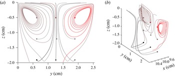
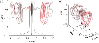
. Figures 11 and 12 depict the trajectories of fluid parcels in a longitudinal plane at
 $x=9.8$
cm (close to the
 $x$
midplane) in the clean and fully contaminated cases respectively. On the other hand, close to the sides of the channel (not shown here), the trajectories are qualitatively similar to those shown with a contaminated interface (figure 12).
Trajectories of fluid parcels starting from various points of the plane
 $x=9.80$
cm (central cell) for
 $m=7$
,
 $2f=10.8$
Hz and
 $A=0.2~\text{cm}^{2}~\text{s}^{-1}$
with a clean interface. (a) Viewed from the face
 $x=L_{x}$
. (b) Slanted view. Each colour denotes the trajectory of the same particle in plots (a) and (b). The starting points of the paths are represented by disks.

Trajectories of fluid parcels starting from various points of the plane
 $x=9.80$
cm (central cell) for
 $m=7$
,
 $2f=10.8$
Hz and
 $A=0.2~\text{cm}^{2}~\text{s}^{-1}$
with a fully contaminated interface. Views and colour conventions are the same as in figure 11.

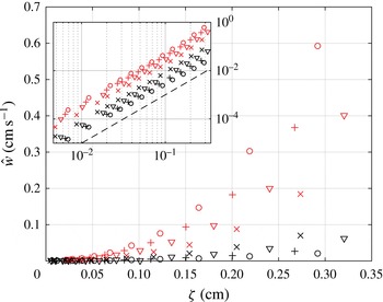
Diagram analogous to figure 4, obtained in this case from numerical simulations: the vertical streaming velocity
 ${\hat{w}}$
, defined in (2.2), increases as a function of the wave amplitude
 $\unicode[STIX]{x1D701}$
. Red symbols represent Faraday streaming flows obtained with a fully contaminated interface, which share most properties of the type-I patterns (rolls). Black symbols stand for Faraday streaming flows obtained with a clean interface that are roughly similar to type-II patterns (swirls). The symbols
 $\times$
, ▿,
 $+$
and ○ correspond to
 $m=4$
, 5, 6 and 7 respectively. The same figure is shown in the inset with a log–log representation. The dashed line at the bottom of the inset has a slope of 2.

In both figures, the
 $y$
midplane, which is a symmetry plane of the problem, plays the role of separatrix between the two halves of the domain: fluid parcels starting within a half stay indefinitely there. The
 $x$
midplane plays the same role of separatrix. A more detailed inspection shows that all of the planes of the equation
 $x=m^{\prime }L_{x}/(2m)$
are separatrices too,
 $m^{\prime }$
being an integer, except those at
 $m^{\prime }=1$
and
 $m^{\prime }=m-1$
in the clean case. Hence, the motion of a fluid particle remains confined to small portions of a box of length
 $L_{x}/(2m)$
and width
 $L_{y}/2$
, depending on its starting point. The separatrices are also visible in figures 5–7 at the locations of vertical streamlines as well as in figure 10 separated by the orthogonal planes of null
 $u$
or
 $v$
components. It is important to emphasise that odd
 $m^{\prime }$
values correspond to nodes of the interface vibration whereas even
 $m^{\prime }$
values correspond to the antinodes. Outside the separatrices, the complexity of the trajectories is mainly illustrated by the paths in the upper part of the domain. For instance, the loops formed by the trajectories in figures 11 and 12 clearly differ: while clean conditions display loops parallel to the
 $x=0$
plane, fully contaminated conditions yield loops parallel to the
 $y=0$
plane. In the case of figure 11, the motion displays a transverse component stronger than the longitudinal one. This is due to the absence of constraints on the velocity field at the top (free tangential-stress/Neumann condition) and the distance from the lateral boundaries. The separatrices disappear when the amplitude increases and the patterns become disordered. In that case, the trajectories of all fluid parcels span the whole domain. All of these assessments indicate that three-dimensional effects on Faraday streaming flows are noticeable, even for longitudinal waves. This contrasts with the weak and local effect of walls on Faraday surface waves.
Finally, we focus on more quantitative aspects of Faraday streaming flows to compare our simulations with the experimental results presented in figure 4. Taking the same definition of the average velocity
 ${\hat{w}}$
as in § 2.4, we plot in figure 13 our numerical results for
 $\widehat{w}$
versus
 $\unicode[STIX]{x1D701}$
as we did for our experiments in figure 4. Different symbols correspond to different
 $m$
values (see caption), while different colours distinguish between patterns obtained with a contaminated surface (in red) and those obtained with a clean surface (in black). We recall that clean-interface patterns share some properties with type-II patterns (swirls), while the contaminated ones remarkably resemble type-I patterns (rolls).
Figures 4 and 13 show interesting similarities. In both cases,
 ${\hat{w}}$
displays small values for
 $\unicode[STIX]{x1D701}<0.15~\text{cm}$
. We also observe fair agreement, as the clean-interface streaming flows generate lower vertically averaged velocities than contaminated streaming flows. The values of
 ${\hat{w}}$
obtained in simulations are remarkably close to those measured in the experiments. However, there is still a qualitative discrepancy between the numerical and experimental diagrams. In experiments, we observe the collapse of the branches of
 ${\hat{w}}$
above the common threshold
 $\unicode[STIX]{x1D701}=\unicode[STIX]{x1D701}_{c}$
. Instead, simulations show scattered branches dependent on
 $m$
, where
 ${\hat{w}}$
increases as
 $\unicode[STIX]{x1D701}^{2}$
, as shown in the inset of figure 13. This feature is directly linked to the boundary-condition dependence on
 $A$
. The origin of this disagreement between numerical and experimental diagrams remains as an open and interesting question. It may come from insufficiently controlled surface properties in the experiment, as well as from the neglect of capillary effects or parasitic circulations in the model.
5 Summary and discussion
In this work, we have studied the steady streaming flows sustained by longitudinal Faraday waves in a rectangular container. We have handled this problem by performing experiments, building a theoretical framework and running numerical simulations.
In the experiments conducted in § 2, we report the observation of streaming flows with a well-resolved spatial structure. These patterns appear at any wavenumber, but their morphology may vary among three types. Type I corresponds to well-defined counter-rotative rolls, type II to moustache-like patterns and type III to irregular patterns. All of these patterns have been observed when performing stroboscopic measurements of tracers, which naturally filter off the periodic motion of standing surface waves. We have obtained the flow streamlines by superposing the sequence of images, and the flow velocity field by performing PIV analysis. Results were summarised in a bifurcation diagram for the streaming vertical velocity as a function of the wave amplitude (figure 4). All of the data collapse into two branches distinguishing type-I patterns (rolls) from type-II (swirls) and type-III (irregular) ones. Furthermore, the type-I and type-II branches coexist in a common range of forcing parameters, which means that identical Faraday waves can sustain qualitatively different streaming flows. Other parameters, such as the wavelength or the bifurcation criticality, do not show any important qualitative role.
We considered a model for the streaming due to oscillatory stationary waves in § 3, which mainly follows Nicolás & Vega (Reference Nicolás and Vega2003) and extends the classic results (cf. Schlichting & Gersten Reference Schlichting and Gersten1999; Batchelor Reference Batchelor2000) to three-dimensional configurations. The theory is based on boundary layers generated by tangential oscillating flows in the vicinity of rigid walls. The equations show that the streaming inside the boundary layer induces a net streaming at the junction with the adjacent outer flow, which can then be used as a matched boundary condition for the bulk. Boundary layers then slowly induce vorticity into the bulk until a steady state – the streaming flow – is attained. Finally, the theoretical framework points out that the boundary layers represent the main source of streaming in the vibrating fluid layer: corrections due to nonlinearities in the bulk are of higher order. Although the process is complex, the final outcome is stunningly simple in terms of equations. For instance, any Navier–Stokes numerical solver can be used to find the steady streaming velocity (without resolving the boundary layers) provided that the right boundary conditions, which have been clearly established, are properly applied.
Focused on our experiments, we have applied this theory to find the streaming induced by the rigid walls in longitudinal Faraday waves in a high-aspect-ratio rectangular container. On the other hand, complementary boundary conditions at the free surface have been fixed accounting for clean and fully contaminated cases. Using the theoretical results, we performed direct numerical simulations aiming to visualise the steady component sustained by Faraday waves. This has been applied to a rectangular domain with a single fluid, where the oscillating Faraday wave and the mean flow only couple through the matched boundary conditions previously presented. From the simulations, we have observed various types of streaming patterns, depending on the surface conditions. In the case of a fully contaminated surface, we have obtained counter-rotative structures that strikingly resemble the type-I patterns (rolls) observed in our experiments. For a clean surface, similarities with type-II experiments (swirls) have also been found although in a less conclusive way. Consideration of conditions of intermediate contamination (Martin & Vega Reference Martin and Vega2005) may improve the agreement with patterns of type II. When we quantified the streaming vertical velocities of the patterns, we found values of the same order of magnitude as in the experiments. Therefore, the results obtained in simulations are compatible with experimental measurements. Then, we have computed a diagram analogous to the experimental one. We have observed that patterns with a contaminated surface and those with a clean surface present distinguishable streaming vertical velocities, recalling the difference among type-I (rolls) and type-II (swirl) patterns in experiments. However, the collapse of the bifurcation diagram found in experiments is replaced in simulations by a dependence on
 $k$
and a quadratic growth when
 $\unicode[STIX]{x1D701}$
increases. This issue deserves further investigation. A rich set of theoretical predictions of secondary bifurcations in various configurations (e.g. annular and small-aspect-ratio containers, pinned-edge waves) that also have an effect on the amplitude of the surface waves (cf. Nicolás & Vega Reference Nicolás and Vega2000; Higuera et al.
Reference Higuera, Vega and Knobloch2002; Martin et al.
Reference Martin, Martel and Vega2002) should be addressed by further experiments. Finally, we have focused on whether the transverse effects are truly negligible. The comparison between three-dimensional streaming flows and two-dimensional ones shows that the walls in the third dimension have an important effect on the streaming flow, remarkably large compared with their effect on surface waves. By computing the horizontal components of the velocity fields and the trajectories of several fluid parcels, we have concluded that a two-dimensional approximation is not sufficient to catch the richness of the flow beneath Faraday waves.
The original investigation of Faraday (Reference Faraday1831) and recent experimental approaches (Falkovich et al. Reference Falkovich, Weinberg, Denissenko and Lukaschuk2005; Sanli et al. Reference Sanli, Lohse and van der Meer2014) have naturally raised a question about how streaming flows may influence the motion of floaters or heavy particles. Although this is out of the scope of the present investigation, our results show that streaming flows are another mechanism leading to slow motion of such particles. Contrary to weight and buoyancy which can only induce vertical motion, the average drag induced by the streaming does contribute with tangential net forces exerted on the particles, even when they are constrained to the bottom or top of the fluid. In particular, the discussed set of separatrices act as basins of repulsion and attraction for particles, whose locations depend on both the wavelength of the Faraday waves and the contamination of the surface. This interesting perspective will be the subject of further exploration.
Finally, the comparison between the numerical and experimental results presented in this work poses an interesting issue. While the numerical results point to the free-surface contamination as the only variable dramatically affecting the streaming flow, the experimental results show that identical Faraday waves sustain qualitatively different streaming flows. To link both results, one may hypothesise a gentle variation in space of the time-averaged surface contamination, rather than assuming it as statically fixing the stress. This scenario has been confirmed recently using new techniques to access the distribution of surfactants (Strickland, Shearer & Daniels Reference Strickland, Shearer and Daniels2015). Evidence points to the fact that contaminants are not just passively dragged by the streaming flow but also exert a feedback on it, a feature that enriches the streaming problem even further.
Acknowledgements
We are very grateful to Professor Edgar Knobloch for his suggestion to study the streaming patterns in Faraday waves, to H. Alarcón, M. Clerc and J. M. Vega for fruitful discussions and comments, and to K. Welch for proofreading our manuscript. L.G. was supported by Conicyt FCHA/Postdoctorado Becas Chile 74160007 and Conicyt PAI/IAC 79160140. P.G. was supported by Conicyt/Fondecyt Postdoctorado 3140550. N.P. was supported by Conicyt/Fondecyt Postdoctorado 3140522. H.U. was supported by Fondecyt 11130450. The laser, the fast camera and some other parts of the set-up were purchased under the funding programme Conicyt AIC-43. Powered@NLHPC: this research was partially supported by the supercomputing infrastructure of the NLHPC (ECM-02).