2.1. Nonlinear Least Squares Solution of Distance Equations

The discussion is started with the following three-dimensional distance equation:

(1) $$L_i =\tilde{L}+\varepsilon_i =d_i (\tilde {{\bf x}})+\varepsilon _i\quad i=1,2,\ldots,n$$

where $d_{i} ({\bf x}):=\sqrt{(x_{1} -y_{i,1} )^{2}+(x_{2} -y_{i,2})^{2}+(x_{3} -y_{i,3})^{2}}$ is the Euclidean distance, $\tilde{{\bf x}}:=\left[ {\tilde {x}_{1} ,\tilde {x}_{2} ,\tilde {x}_{3} } \right] $ is the unknown position, ${\bf y}_{i} :=\left[ {y_{i,1} ,y_{i,2} ,y_{i,3} } \right] $ is the ith known position, L _i is the distance observation, $\tilde{L}_i$ is the true distance, and $\varepsilon _{i}$ is the observation error. Let $\hat{{\bf x}}$ be the least squares solution of Equation (1), then the so-called orthogonality condition is satisfied (Xue et al., Reference Xue, Yang and Dang2014b) as

(2) $${{\bf h}}(\hat{{\bf x}})={{\bf J}}^{\rm T}(\hat{{\bf x}}) {{\bf PV}}(\hat{{\bf x}})={{\bf 0}}$$

where ${{\bf P}}=diag[p_{1} ,p_{2} ,\ldots,p_{n}]>0$ is the weight matrix,

(3) $${{\bf J}}(\hat{{\bf x}}):=\left[ {{\matrix{ {{{\bf j}}_1^{{\rm T}} ({{\hat{{\bf x}}}})} & {{{\bf j}}_2^{\rm T} ({{\hat{{\bf x}}}})} & \cdots & {{{\bf j}}_n^{\rm T} ({{\hat{{\bf x}}}})} } }} \right]^{\rm T}$$

is the Jacobian matrix, ${{\bf j}}_{i} ({{\hat{{\bf x}}}})=\left[ {{\matrix{ {\hat{{x}}_{1} -y_{i,1} } & {\hat{{x}}_{2} -y_{i,2}} & {\hat{{x}}_{3} -y_{i,3}} } }} \right]/d_{i} ({{\hat {{\bf x}}}})$ is the line of sight from the unknown point to the ith known point,

(4) $${\bf V}(\hat {{\bf x}})={\bf L}-{\bf d}(\hat {{\bf x}})$$

is the residual vector, ${\bf d}(\hat{{\bf x}})=\left[ {{\matrix{ {d_{1} (\hat{{\bf x}})} & {d_{2} (\hat{{\bf x}})} & \cdots & {d_{n} (\hat{{\bf x}})} } }} \right]^{\rm T}$ , and ${\bf L}=\left[ {{\matrix{ {L_{1} } & {L_{2} } & \cdots & {L_{n} } } }} \right]^{\rm T}$ .

The nonlinear least squares solution in Equation (2) is generally difficult to determine analytically, but it can be locally iteratively solved by the Newton method of the form

(5) $${{\hat{{\bf x}}}}_{k+1} ={{\hat{{\bf x}}}}_k +{{\bf H}}^{-1}({{\hat{{\bf x}}}}_k ){{\bf h}}({{\hat{{\bf x}}}}_k )$$

if the Hessian matrix

(6) $${{\bf H}}({{\hat{{\bf x}}}})=\left. {{\partial {{\bf h}}({{\bf x}}) \over \partial {\bf x}}} \right\vert_{{{\hat{{\bf x}}}}} ={{\bf N}}({{\hat{{\bf x}}}})+{{\bf S}}({{\hat{{\bf x}}}})$$

is positive, where

(7) $${{\bf N}}({{\bf x}}):={{\bf J}}^{\rm T}({{\bf x}}){{\bf PJ}}({{\bf x}})$$

is the normal matrix of the linearization of Equation (1),

(8) $${{\bf S}}({{\bf x}}):=\sum\limits_{i=1}^n {V_i ({{\bf x}}_i )p_i {{\bf G}}_i ({{\bf x}})}$$

is the term related to the size of residual and the second-order derivatives,

(9) $$\eqalign{{\bf G}_i ({\bf x})&:= \displaystyle{\partial d_i^2 ({\bf x}) \over \partial^2{\bf x}} = \left[{\bf I} - {\bf j}_i^{\rm T} ({\bf x}) {\bf j}_i({\bf x}) \right] /d_i ({\bf x}) \cr &=\left[\matrix{ \displaystyle{1 \over d_i {\bf x}}- \displaystyle{(x_1 -y_{i,1})^2 \over d_i^3 ({\bf x})} & \displaystyle{- (x_1 - y_{i,1}) (x_2 - y_{i,2}) \over d_i^3 ({\bf x})} & \displaystyle{- (x_1 - y_{i,1})(x_3 - y_{i,3}) \over d_i^3 ({\bf x})} \cr \displaystyle{- (x_2 -y_j) (x_1 - y_{i,1}) \over d_i^3} & \displaystyle{1 \over d_i ({\bf x})}- \displaystyle{(x_2 -y_{i,2})^2 \over d_i^3 ({\bf x})} & \displaystyle{- (x_2 - y_j) (x_3 - y_{i,3}) \over d_i^3 ({\bf x})} \cr \displaystyle{- (x_3 - y_{i,3}) (x_1 - y_{i,1}) \over d_i^3 ({\bf x})} & \displaystyle{- (x_3 - y_{i,3}) (x_2 - y_{i,2}) \over d_i^3 ({\bf x})} & \displaystyle{1 \over d_i ({\bf x}} - \displaystyle{(x_3 -y_{i,3})^2 \over d_i^3 ({\bf x})}} \right]}$$

where ${{\bf I}}\in \Re ^{3\times 3}$ is the identity matrix.

Ignoring the term Equation (8) in the Newton method, we can obtain the Gauss-Newton method for iteratively solving the distance equations. For short-distance observations of low precision, the Newton method has a high convergence speed and high success rate, and it can be expressed in a closed form to save computational cost (Xue et al., Reference Xue, Yang and Dang2014b). When there are linear nuisance parameters (such as the clock offset) in Equation (1), which need to be estimated, the proposed results can be generalised because the linearization remainder is only related to the distance equations.

2.2. Bias in the Nonlinear Least Squares Solution

The nonlinear least squares solution is generally biased and the bias vector can be defined as

(10) $$\tilde {\Delta }=E({{\hat{{\bf x}}}})-{{\tilde{{\bf x}}}}$$

where ${{\tilde{{\bf x}}}}$ is the true position,

(11) $$E(\hat{{\bf x}})=\int \int \int_{L\in \Re^n} {{\bf p}({\bf L})d\Theta ({\bf L})}$$

is the mathematical expectation of the nonlinear least squares solution, and

(12) $$\hat{{\bf x}}={\bf p}({\bf L})$$

implicitly or explicitly is given by the orthogonality condition Equation (2), and $\Theta ({\bf L})$ is the probability distribution of observation. The variance of the nonlinear least squares solution can be defined as

(13) $${{\bf D}}_{{{\hat{{\bf x}}}}} =E\left\{ {\left[ {{{\hat{{\bf x}}}}-E({{\hat{{\bf x}}}})} \right] \left[ {{{\hat{{\bf x}}}}-E({{\hat{{\bf x}}}})} \right]^{\rm T}} \right\} =\int \int \int_{{{{\bf L}}\in \Re ^n}} {\left[ {{{\hat{{\bf x}}}}-E({{\hat{{\bf x}}}})} \right] \left[ {{{\hat{{\bf x}}}}-E({{\hat{{\bf x}}}})} \right]^{\rm T}d \Theta ({{\bf L}})}$$

Using the bias, the unbiased nonlinear least squares solution can be defined as

(14) $$\mathop{\bf x}\limits^{\frown} = \hat{{\bf x}}-\tilde{\Delta}$$

Particularly for Equation (12), which is explicitly given, integrals Equations (11) and (13) are relatively easy to calculate, compare with Jeudy (Reference Jeudy1988). In general, the nonlinear least squares solution cannot be explicitly given; thus, hereafter, we apply the Monte Carlo method to solve this problem. The probability density of observational errors needs to be assumed prior to applying the Monte Carlo method, such as the commonly used normal distribution (Leick, Reference Leick2004):

(15) $$g({{\bf \rvarepsilon }})= {{1}\over \sqrt {{(2}\pi)^n\det {{\bf D}}_{\bf L} } }e^{-{{1} \over {2}}{{\bf \rvarepsilon }}^{\rm T}{{\bf D}}_{{\bf L}}^{-1} {{\bf \rvarepsilon }}}$$

where ${{\bf D}}_{\bf L} ={{\bf P}}^{-1}\sigma _{0}^{2} $ is the variance of observations, $\sigma _{0}^{2} $ is the variance of unit weight. Then, for the true position ${{\tilde{{\bf x}}}}$ and the distances ${{\tilde{{\bf L}}}}={{\bf d}}({{\tilde{{\bf x}}}})$ given, we can obtain N variates from the random variable ${{\bf L}}={{\tilde {{\bf L}}}}+{{\bf \rvarepsilon }}$ as follows

(16) $$\left\{\matrix{{\bf L}_1 ={\tilde{{\bf L}}}+{{\bf \rvarepsilon }}_1 , \cr {\bf L}_2 ={\tilde{{\bf L}}}+{{\bf \rvarepsilon }}_2 \cr \quad \,\vdots \cr {\bf L}_N ={\tilde{{\bf L}}}+{{\bf \rvarepsilon }}_N} \right.$$

where ${{\bf \rvarepsilon }}_{1},{{\bf \rvarepsilon }}_{2},\ldots,{{\bf \rvarepsilon }}_{N}$ follow the assumed probability distribution, such as Equation (15). Using the variates in Equation (16), we can obtain N solutions

(17) $$\left\{\matrix{\hat{{\bf x}}_1 ={{\bf p}}({\bf L}_1 ) \cr \hat{{\bf x}}_2 ={{\bf p}}({\bf L}_2 ) \cr ,\ldots , \cr \hat{{\bf x}}_N ={{\bf p}}({\bf L}_N )}\right.$$

with the Newton or Gauss-Newton method. For a sufficiently large number N, the bias Equation (10) can then be accurately estimated by

(18) $${{\hat{{\bf \Delta}}}}={\sum\limits_{i=1}^N {{{\hat{{\bf x}}}}_i } }\Bigg/N-{\tilde{{\bf x}}}$$

Accordingly, the variance can be estimated by

(19) $$\hat {\sigma }_{i,\,j}= {\sum_{k=1}^N {\left[ {\hat{{x}}_{k,i} -\hat {\Delta }_i -\tilde {x}_i } \right] \left[ {\hat{{x}}_{k,j} -\hat {\Delta }_j -\tilde {x}_j } \right] } \over N-1}$$

where the denominator N−1 guarantees the optimality of the estimation.

However, in most cases, we only have variance about the observation errors, and studies suggest that normally distributed errors do not represent true errors. Moreover, the computational cost of the Monte Carlo method is very high, especially for large dimension observations. Therefore, bias and variance estimations based on the linearization adjustment will be discussed.

3.1. Variance Estimation

Given $\hat{{\bf x}}_{0}$ is the initial value, we can obtain an equivalent model of Equation (1) according to Taylor's theorem as follows

(20) $${{\bf J}}({{\hat{{\bf x}}}}_0)\hbox{d}{{\bf x}}={{\bf V}}({{\hat{{\bf x}}}}_0 )-{{\bf r}}_1$$

where $\hbox{d}{\bf x}={\bf x}-\hat{{\bf x}}_{0}$ ,

(21) $${{\bf r}}_1 = {1 \over 2}\left[ {{\matrix{ {\hbox{d}{{\bf x}}^{\rm T}{\bf G}_1 ({{\hat{{\bf x}}}}_0 +\theta_1 \hbox{d}{{\bf x}})\hbox{d}{{\bf x}}} & {\hbox{d}{{\bf x}}^{\rm T}{\bf G}_2 ({{\hat{{\bf x}}}}_0 +\theta_2 \hbox{d}{{\bf x}})\hbox{d}{{\bf x}}} & \cdots & {\hbox{d}{{\bf x}}^{\rm T}{\bf G}_n ({{\hat{{\bf x}}}}_0 +\theta_n \hbox{d}{{\bf x}})\hbox{d}{{\bf x}}}} }} \right]^{\rm T}$$

$\theta _{i} \in [ {0,1}]$ . Because $\theta _{i}\ (i=1,2,\ldots,n)$ is unknown, traditionally the second-order remainders in Equation (21) are left in the random model, i.e., they are treated as random error sources. However, the remainder is a positive quantity because the following inequality holds (Xue et al., Reference Xue, Yang and Dang2014a)

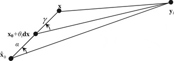
(22) $$\eqalign{r_{1,i} &=\hbox{d}{\bf x}^{\rm T} G_i (\hat{{\bf x}}_0 +\theta_i\hbox{d}{\bf x})\hbox{d}{\bf x} = {\hbox{d}{\bf x}^{\rm T}\lpar {{\bf I}-{\bf j}^{\rm T}(\hat{{\bf x}}_0 +\theta_i \hbox{d}{\bf x}){\bf j}(\hat{{\bf x}}_0 +\theta_i \hbox{d}{\bf x})} \rpar \hbox{d}{\bf x} \over \hbox{d}(\hat{{\bf x}}_0+\alpha \hbox{d}{\bf x})} \cr & = \Vert {\hbox{d}{\bf x}}\Vert_2^2 \sin^2\gamma/\Vert {{\bf y}_i -\hat{{\bf x}}_0 -\theta _i \hbox{d}{\bf x}}\Vert_{2} \cr &\ge 0}$$

For relatively small values of $\Vert {\hbox{d}{\bf x}} \Vert$ , we have the following approximation

(23) $$r_{1,i} \approx {\hbox{d}{\bf x}^{\rm T}( {{\bf I}-{{\bf j}}_i^{\rm T} ({{\bf x}}){{\bf j}}_i({{\bf x}})})\hbox{d}{\bf x} \over d(\hat{{\bf x}}_0)} = {\Vert {\hbox{d}{\bf x}} \Vert_2^2 \sin ^2\alpha}/{\Vert {{\bf y}_i - \hat{{\bf x}}_0} \Vert_2 }$$

where α is the intersection angle between the error direction $\hbox{d}{{\bf x}}={{\bf x}}-{{\hat{{\bf x}}}}_{0} $ and the line of sight ${{\bf j}}_{i}({{\hat{{\bf x}}}}_{0})$ . The geometrical definitions of the quantities in Equations (22) and (23) are illustrated in Figure 1. Accordingly, the remainders in Equation (22) are indeed systematic errors. In Section 3.2, statistical characteristics of the remainders are discussed to improve the linearization adjustment.

Figure 1.

Geometrical meaning of Nonlinearity remainder.

Coming back to model Equation (20), by ignoring the first-order remainder vector in Equation (20), we can obtain the following linearization model

(24) $${{\bf J}}({{\hat{{\bf x}}}}_0 ){\hbox{d}{\bf x}}={{\bf V}}({{\hat{{\bf x}}}}_0 )$$

and the least squares solution based on the linearization Equation (24) reads

(25) $${{\hat{{\bf x}}}}^G ={{\hat{{\bf x}}}}_0+\hat{{\rm d}}{{\bf x}}^G$$

where

(26) $$\hat{{\rm d}}{{\bf x}}^G ={{\bf N}}^{-1}({{\hat{{\bf x}}}}_0){{\bf h}}({{\hat{{\bf x}}}}_0)$$

is the least squares solution of Equation (20), i.e., the one step iterative solution from the Gauss-Newton method. When $\hat{{\bf x}}_{0}$ is inaccurate, the solution Equation (25) can then be iteratively improved using the Gauss-Newton method as

(27) $${{\hat{{\bf x}}}}_{k+1}^G ={{\hat{{\bf x}}}}_k^G +{{\bf N}}^{-1}({{\hat{{\bf x}}}}_k^G ){{\bf h}}({{\hat{{\bf x}}}}_k^G )$$

By applying the error propagation to Equation (25), the variance estimation of ${{\hat{{\bf x}}}}^{G}$ reads

(28) $$\eqalign{{{\hat{{\bf D}}}}_{{{\hat{{\bf x}}}}^G }&:=\hbox{cov}({{\hat{{\bf x}}}}^G) \cr &=\hbox{cov}({{\hat{{\bf x}}}}_0 )+\hbox{cov}(\hat {\hbox{d}}{{\bf x}}^G) \cr & = E \left[ {(\hat {\hbox{d}}{{\bf x}}^G)(\hat {\hbox{d}}{{\bf x}}^G)^{\rm T}} \right] -E(\hat {\hbox{d}}{{\bf x}}^G)E^{\rm T}(\hat {\hbox{d}}{{\bf x}}^G)}$$

where E() is the mathematical expectation, and $\hbox{cov}({{\hat{{\bf x}}}}_{0})=0$ for the constant value of $\hat{{\bf x}}_{0}$ . Traditionally, it is assumed that $E(\hat {\hbox{d}}{{\bf x}}^{G})=0$ , which leads to the following approximation

(29) $${{\hat{{\bf D}}}}_{{{\hat{{\bf x}}}}^G}=E\left[ {(\hat{{\rm d}}{{\bf x}}^G)(\hat{{\rm d}}{{\bf x}}^G)^{\rm T}} \right] ={{\bf N}}^{-1}({{\hat{{\bf x}}}}_k^G ){{\bf J}}^{\rm T}({{\hat{{\bf x}}}}_k^G ){{\bf P}}({{\bf P}}^{-1}\sigma _0^2 ){{\bf PJ}}({{\hat{{\bf x}}}}_k^G ){{\bf N}}^{-1}({{\hat{{\bf x}}}}_k^G )={{\bf N}}^{-1}({{\hat{{\bf x}}}}_0)\sigma _0^2$$

Generally, ${{\hat{{\bf x}}}}_{k+1}^{G} $ , i.e., the solution from the Gauss-Newton method, can converge to the nonlinear least squares solution for a sufficiently large k, ${{\hat{{\bf x}}}}_{\infty}^{G} ={{\hat{{\bf x}}}}$ , compare with Teunissen (Reference Teunissen1990b). In this case, the variance estimation Equation (29) converges to the following estimation

(30) $${{\hat{{\bf D}}}}_{{{\hat{{\bf x}}}}}={{\bf N}}^{-1}({{\hat{{\bf x}}}})\sigma _0^2$$

When there is no prior information about the variance of unit weight, the variance of observations can be estimated by

(31) $${{\hat{{\bf D}}}}_{{\bf L}}={{\bf P}}^{-1}\hat{\sigma}_0^2 ({{\hat{{\bf x}}}}_k^G)$$

where

(32) $$\hat {\sigma }_0^2 ({{\hat{{\bf x}}}}_k^G )={{{\bf V}}^{\rm T}({{\hat{{\bf x}}}}_k^G ){{\bf PV}}({{\hat{{\bf x}}}}_k^G )}/{(n-3)}$$

is the posterior variance of unit weight, and for k→∞, the variance estimation Equation (32) converges to the estimation

(33) $${{\hat{{\bf D}}}}_{{\bf L}}={{\bf P}}^{-1}\hat {\sigma }_0^2({{\hat{{\bf x}}}})$$

with $\hat {\sigma }_{0}^{2} ({{\hat{{\bf x}}}})={{{\bf V}}^{\rm T}({{\hat{{\bf x}}}}){{\bf PV}}({{\hat{{\bf x}}}})}/{(n-3)}$ .

Because the second-order derivatives in Equation (9) are omitted, the variance estimation based on the linearization model may be inaccurate in the linearization adjustment model, especially in case of low precision of short-distance observations. The bias in the nonlinear least squares solution can result in the possibility that the traditional variance estimation Equation (30) based on the nonlinear least squares solution might be inaccurate. One way to solve this problem is to estimate the bias of the nonlinear least squares solution.

3.2. Bias Estimation and Updated Variance Estimations

According to the model Equation (20), which is equivalent to Equation (2), we have

(34) $${{\bf J}}({{\hat{{\bf x}}}}_0 )E(\hbox{d}{{\bf x}})=E \left[ {{{\bf V}}({{\hat{{\bf x}}}}_0 )} \right] -E({{\bf r}}_1 )$$

where

(35) $${\bf r}_1 = {1 \over 2} \left[\matrix{\hbox{d} {\bf x}^{\rm T}{\bf G}_1 (\hat{\bf x}_0) \hbox{d} {\bf x} &\hbox{d} {\bf x}^{\rm T}{\bf G}_2 (\hat{\bf x}_0) \hbox{d} {\bf x} & \cdots & \hbox{d} {\bf x}^{\rm T} {\bf G}_n (\hat{\bf x}_0) \hbox{d}{\bf x}} \right]^{\rm T}+ {\bf r}_2$$

and ${{\bf r}}_{2} $ contains the second-order remainders of the linearization. Generally, ${{\bf r}}_{2} $ can be ignored because it is proportional to $d^{-3} ({{\bf x}})$ . Then, let ${\bf D}_{x_{0} } $ be the variance of ${{\hat{{\bf x}}}}_{0} $ ; applying the expectation theorem of the quadratic form to Equation (22) (Mathai and Provost, Reference Mathai and Provost1992), the second-order approximation for $E({{\bf r}}_{1} )$ reads

(36) $$\eqalign{\tilde {{\bf b}}&:=E({{\bf r}}_1 )\approx {1 \over 2}E\left[ {{\matrix{ {\hbox{d}{{\bf x}}^{\rm T}{\bf G}_1 ({{\hat{{\bf x}}}}_0 )\hbox{d}{{\bf x}}} & {\hbox{d}{{\bf x}}^{\rm T}{\bf G}_2 ({{\hat{{\bf x}}}}_0 )\hbox{d}{{\bf x}}} & \cdots & {\hbox{d}{{\bf x}}^{\rm T}{\bf G}_n ({{\hat{{\bf x}}}}_0 )\hbox{d}{{\bf x}}} \cr} }} \right]^{\rm T} \cr &= {1 \over 2}\left[ {{\matrix{ {tr\lpar {{\bf D}_{{\bf x}_0 } {\bf G}_1 ({{\hat{{\bf x}}}}_0 )} \rpar } & {tr\lpar {{\bf D}_{{\bf x}_0 } {\bf G}_2 ({{\hat{{\bf x}}}}_0 )} \rpar } & \cdots & {tr\lpar {{\bf D}_{{\bf x}_0 } {\bf G}_n ({{\hat{{\bf x}}}}_0 )} \rpar }} }} \right]^{\rm T}}$$

where tr(•) is the trace of the matrix.

When there is no prior information about the precision of the initial value, i.e., when ${\bf D}_{{\bf x}_{0}}$ is unknown, nonlinear least squares estimations can be used as initial conditions to estimate the bias Equation (36), that is,

(37) $$\tilde {{\bf b}}\approx \hat {{\bf b}}:= {1 \over 2}\left[ {{\matrix{ {tr( {{\bf D}_{\hat{{\bf x}}} {\bf G}_1 (\hat{{\bf x}})} )} & {tr( {{\bf D}_{\hat{{\bf x}}} {\bf G}_2 (\hat{{\bf x}})} )} & \cdots & {tr( {{\bf D}_{\hat{{\bf x}}} {\bf G}_n (\hat{{\bf x}})} )}} }} \right]^{\rm T}$$

where ${\bf D}_{\hat{{\bf x}}} $ and $\hat{{\bf x}}$ are the nonlinear least squares estimations. If $\hat{\bf b}_i$ is the ith entry of Equation (37), the following inequality holds

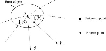
(38) $$\eqalign{\hat{{b}}_i &= {1 \over 2}E\left[ {\hbox{d}{{\bf x}}^{\rm T}{\bf G}_i ({{\hat{{\bf x}}}})\hbox{d}{{\bf x}}} \right] \cr &= {E\left[ {\hbox{d}{{\bf x}}^{\rm T}\hbox{d}{{\bf x}}} \right] -{{\bf j}}_i^{\rm T} (\hat{{\bf x}})E\left[ {\hbox{d}{{\bf x}}^{\rm T}\hbox{d}{{\bf x}}} \right] {{\bf j}}_i(\hat{{\bf x}}) \over 2d_i (\hat{{\bf x}})} \cr &= {tr({\bf D}_{\hat{{\bf x}}} )-{{\bf j}}_i^{\rm T} (\hat{{\bf x}}){{\bf D}}_{\hat{{\bf x}}}{{\bf j}}_i(\hat{{\bf x}}) \over {2}d_i (\hat{{\bf x}})} \cr &= {tr({{\bf D}}_{\hat{{\bf x}}} )-\sigma _{{{\bf j}}_i }^2 \over {2}d_i(\hat{{\bf x}})} \cr &\ge 0}$$

where

(39) $$\sigma _{{{\bf j}}_i }^2 ={{\bf j}}_i^{\rm T} (\hat{{\bf x}})\hbox{D}_{\hat{{\bf x}}} {{\bf j}}_i(\hat{{\bf x}})$$

is the directional variance along the line of sight as shown in Figure 2, compare with Seemkooei (Reference Seemkooei1998, p. 15). The inequality Equation (38) is given a statistical meaning corresponding to the inequality Equation (22), and the equality in Equation (38) provides a statistical model for improving the traditional linearization model.

Figure 2.

Geometrical meaning of the bias in distance estimations.

The above-mentioned discussions indicate that the unbiased parameters can result in a statistical bias in the first-order remainder vector Equation (21), i.e., in the distance prediction ${\bf d}(\hat{{\bf x}})$ . To compensate for the bias, the following adjustment model needs to be introduced

(40) $${{\bf J}}({{\hat{{\bf x}}}}_0 ){\rm d}{{\bf x}}={{\bf V}}({{\hat{{\bf x}}}}_0 )+\hat{{\bf b}}$$

and then the least squares solution of Equation (40) is close to becoming unbiased; it reads

(41) $${\mathop{\bf x}\limits^{\frown}}^G ={{\hat{{\bf x}}}}_0 +{{\bf N}}^{-1}({{\hat{{\bf x}}}}_0 ){{\bf h}}({{\hat{{\bf x}}}}_0 )+{{\bf N}}^{-1}({{\hat{{\bf x}}}}_0 ){{\bf J}}^{\rm T}({{\hat{{\bf x}}}}_0 )\hat {{\bf b}}$$

For the initial value $\hat{{\bf x}}_{0}$ of low precision, the iterative solution for ${\mathop{\bf x}\limits^{\frown}}$ reads

(42) $${\mathop{\bf x}\limits^{\frown}}_{k+1}={{\hat{{\bf x}}}}_k+{{\bf N}}^{-1}({{\hat{{\bf x}}}}_k ){{\bf J}}^{\rm T}({{\hat{{\bf x}}}}_k )\hat {{\bf b}}$$

As, k→∞ in general, Equation (42) can converge to the following solution

(43) $${{\mathop{\bf x}\limits^{\frown}}}_{\infty} ={{\hat{{\bf x}}}}-{{\bf \Delta }}^G$$

where ${{\hat{{\bf x}}}}$ is the nonlinear least squares solution,

(44) $${{\bf \Delta }}^G =-{{\bf N}}^{-1}({{\hat{{\bf x}}}}){{\bf J}}^{\rm T}({{\hat{{\bf x}}}}){{\bf P}}\hat {b}$$

is the bias estimation based on the linearization adjustment model.

Coming back to Equation (20), generally the LS residual vector is biased because of the linearization reminder ${{\bf r}}_{1} $ , which might lead to a bias in the LS variance Equation (32) of unit weight. By applying the bias estimation Equation (37) to Equation (29) and using the unbiased parameters we can obtain the variance estimation as follows

(45) $${\mathop{\bf D}\limits^{\frown}}_{{\mathop{\bf x}\limits^{\frown}}} ={{\bf N}}^{-1}({\mathop{\bf x}\limits^{\frown}}) {\mathop{\sigma}\limits^{\frown}}_0^2$$

where the unbiased variance estimation of unit weight can then be updated using

(46) $${\mathop{\sigma}\limits^{\frown}}_0^2 ={{{\bf V}}^{\rm T}({\mathop{\bf x}\limits^{\frown}}){{\bf V}}({\mathop{\bf x}\limits^{\frown}})}/{(n-3)}$$

Besides, based on the LS solution we have ${\mathop{\sigma}\limits^{\frown}}_{0}^{2} =[{{\bf V}}({{\hat{{\bf x}}}})-{{\bf {b}}}']^{\rm T}[{{\bf V}}({{\hat{{\bf x}}}})-{{\bf {b}}}']$ where ${{\bf {b}}}'=({{\bf I}}-{{\bf J}}({{\hat{{\bf x}}}}){{\bf N}}^{-1}({{\hat{{\bf x}}}}){{\bf J}}^{\rm T}({{\hat{{\bf x}}}}){{\bf P}}){{\hat{{\bf b}}}}$ is the orthogonal projection of ${{\hat{{\bf b}}}}$ in the observational space, compare with Teunissen (Reference Teunissen1990a, Equation 40).

Equation (38) shows that the positive bias $\hat{b}_i$ is inversely proportional to the distance from the known point to the unknown point. Thus, the positional bias Equation (44) will be small if all the elements of $\hat{{\bf b}}$ are sufficiently close to zero, so that the model is essentially linear, or if $\hat{{\bf b}}$ is orthogonal to the column space of ${{\bf J}}(\hat{{\bf x}})$ so that ${{\bf J}}^{\rm T}(\hat{{\bf x}})\hat{{\bf b}}={\bf 0}$ . The scaled measure $\left[ {({{\bf \Delta }}_{0}^{G} )^{\rm T}{{\bf J}}^{\rm T}({{\hat{{\bf x}}}}){{\bf PJ}}({{\hat{{\bf x}}}}){{\bf \Delta}}_{0}^{G} } \right] /3\hat {\sigma }_{0}^{2} ({{\hat{{\bf x}}}})$ can be used to measure the size of the bias, and it is connected with the parameter-effects curvature of the model nonlinearity (Bates and Watts, Reference Bates and Watts1980; Box, Reference Box1971; Cook et al., Reference Cook, Tsai and Wei1986).

For the distance observation model shown in Figure 2, when the distance $\tilde{L}_{i} $ from the ith known point ${{\bf y}}_{i} $ to the unknown point x is long enough or when the error ellipsoid of the positional parameters is small enough, the probability of the point x lying within the sphere $\{ {{\bf x}\vert \Vert {{\bf x}-\tilde {{\bf y}}_{i} } \Vert \le L_{i} } \}$ is close to 0.5, such that the distance bias $\hat{\bf b}_i$ tends to be 0. In addition, when known points are randomly and uniformly distributed in the three-dimensional space, i.e., the positioning configuration has the lowest GDOP, we have ${{\bf J}}^{\rm T}(\hat{{\bf x}})\hat{{\bf b}}={{\bf 0}}$ to guarantee the unbiasedness.

3.3. Iterative procedure for Unbiased Nonlinear Least Squares

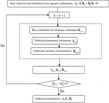
As discussed in Sections 3.1 and 3.2, the initial variance estimation Equation (30) used in Equation (37) for estimating the bias in the nonlinear least squares solution is based on the biased nonlinear least squares. Thus, an iterative procedure to obtain the unbiased nonlinear least squares is needed and is given in Figure 3. The procedure starts with the nonlinear least squares estimations as initial values. Then, the following quantities are iteratively calculated in the proposed procedure:

(47) $$\eqalign{\hat{{\bf b}}_{k+1} &={1 \over 2}\left[ {{\matrix{ {tr\lpar {{\bf D}_{{\mathop{\bf x}\limits^{\frown}},k} {\bf G}_1 ({{\mathop{\bf x}\limits^{\frown}}}_k )} \rpar } & {tr\lpar {{\bf D}_{{{\mathop{\bf x}\limits^{\frown}}},k} {\bf G}_2 ({{\mathop{\bf x}\limits^{\frown}}}_k )} \rpar } & \cdots & {tr\lpar {{\bf D}_{{{\mathop{\bf x}\limits^{\frown}}},k} {\bf G}_n ({{\mathop{\bf x}\limits^{\frown}}}_k )} \rpar } \cr} }} \right]^{\rm T} \cr {{\mathop{\bf x}\limits^{\frown}}}_{k+1}&={{\hat{{\bf x}}}}+{{\bf N}}^{-1} ({{\mathop{\bf x}\limits^{\frown}}}_k ){{\bf J}}^{\rm T} ({{\mathop{\bf x}\limits^{\frown}}}_k )\hat {{\bf b}}_{k+1} \cr {\mathop{\bf D}\limits^{\frown}}_{{\mathop{\bf x}\limits^{\frown}},k} &={{\bf N}}^{-1}({{\mathop{\bf x}\limits^{\frown}}}_k) {\mathop{\sigma}\limits^{\frown}}_{0,k}^2}$$

and

(48) $${\mathop{\sigma}\limits^{\frown}}_{0,k}^2 ={\left[ {{{\bf V}}({{\mathop{\bf x}\limits^{\frown}}}_k )-\hat {{\bf b}}_k } \right]^{\rm T}\left[ {{{\bf V}}({{\mathop{\bf x}\limits^{\frown}}}_k )-\hat {{\bf b}}_k } \right] }\bigg{/}{(n-3)}$$

where ${{\mathop{\bf x}\limits^{\frown}}}_{0} ={{\hat{{\bf x}}}}$ and $\hat {{\bf b}}_{0} =0$ are the initial values for starting the iteration.

Figure 3.

Iterative procedure for unbiased nonlinear least squares estimations.

4.1. Simulation Verification

4.1.1. Positioning configuration simulation

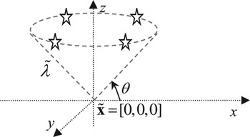
As shown in Figure 4, a cone configuration composed of eight control points is simulated to verify the main results proposed. The unknown position is located at $\left[0m, 0m, 0m \right]^{\rm T}$ , and the distance equations are simulated as follows:

(49) $$\eqalign{&\sqrt {(x-\tilde {\lambda }\cos (2i\pi /8)\cos \theta )^2+(y-\tilde {\lambda }\sin (2i\pi /8)\cos \theta )^2+(z-\tilde {\lambda }\sin \theta )^2} =\tilde {\lambda }+\varepsilon _i \cr &\quad i=1,2,\ldots,8}$$

where θ determines the size of the cone angle, $\tilde {\lambda }$ is the true value of the distance from the unknown point to the known points, and $\varepsilon _{i} $ is the observational error simulated by the normal distribution of variance 1m as follows

(50) $$g({{\bf \rvarepsilon }})= {{1} \over \sqrt {{2}\pi }}e^{-{{1} \over {2}}{{\bf \rvarepsilon }}^{\rm T}{{\bf \rvarepsilon }}}$$

Namely, ${\bf D}_{{\bf \rvarepsilon }} ={\bf I}$ .

Figure 4.

Cone configuration.

For each fixed combination $(\theta ,\tilde {\lambda })$ , the observational model Equation (49) is simulated N=100,000 times for detecting the bias in the nonlinear least squares estimations.

4.1.2. Bias estimation based on the Monte Carlo method

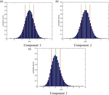
For each fixed combination $(\theta ,\tilde {\lambda })$ , 100,000 simulated distance equations of Section 4.1 are solved by the Newton method, and the bias in the nonlinear least squares solution is estimated by Equation (17). It is shown that the coordinate components $\hat{x} \hbox{and} \hat{y}$ are unbiased because the linearization remainder vector is orthogonal to the xoy range space of the design matrix. This unbiased condition has been discussed in general in Section 3. However, the coordinate component $\hat{z}$ is biased. To show this, only two cases are given as follows:

1. (a) In case of the combination $(\theta ,\tilde{\lambda})=(30^{\circ} ,10\hbox{m})$ , we obtain $\Delta_{1} =[{-}0.003486 \quad {-}0.000860 \quad 0.086329]\hbox{m}$ . The frequency histograms of the nonlinear least squares solutions are given in Figure 5.

2. (b) In case of the combination of $(\theta ,\tilde {\lambda })=(60^{\circ} ,50\hbox{m})$ , we obtain the bias $\Delta _{1} =[-0.000775 \quad 0.009413 \quad 0.022051] \hbox{m}$ .

Figure 5.

Frequency histogram of nonlinear least squares solutions.

4.1.3. Bias estimation based on the proposed iterative procedure

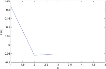
To show the convergence of the proposed iterative procedure, we use the distance observations ${\bf L}=[7.98,\,10.72,\,9.44,\,10.77,\,10.36,\,11.80,\,11.53,\,9.81]^{\rm T}\hbox{m}$ from combination $(\theta, \tilde{\lambda})=(70^{\circ}, 10\,\hbox{m})$ as an example. For this example with $\Vert {{{\mathop{\bf x}\limits^{\frown}}}_{k+1} -{{\mathop{\bf x}\limits^{\frown}}}_{k} }\Vert \le 0.0001$ , the iteration sequence in the z coordinate component is given in Figure 6. This shows convergence to the solution ${{\hat{{\bf x}}}}=[2.919045,\,1.501054,\,-0.051657]^{\rm T}$ after five iteration steps, which is more accurate than the nonlinear least squares solution ${{\hat{{\bf x}}}}=[2.924039, 1.511619, 0.221450]^{\rm T}$ .

Figure 6.

Iteration sequence in z coordinate component.

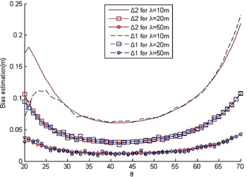
Given $\tilde {\lambda }=10\hbox{m},20\hbox{m},50\hbox{m}$ and $\theta =20^{\circ} ,21^{\circ} ,\ldots,70^{\circ} $ , the bias estimations for the z coordinate component of the least squares solution (Figure 7) are given as follows:

1. (a) Δ₁ estimated by Equation (18) from the Monte Carlo method;

2. (b) Δ₂ estimated by the iterative procedure proposed in Section 3.

Figure 7.

Bias in z component of the nonlinear least squares.

As shown in Figure 7, the proposed bias estimation Δ₂ is as accurate as the bias estimation Δ₁ based on a large number of random variates. Figure 7 shows that the bias is inversely proportional to the distance $\tilde{\lambda}$ and is also related to the size of the cone angle, i.e., the size of the PDOP. This indicates that the bias is relatively small for the positioning configuration with the lowest PDOP. The bias estimation Δ₂ derivates from the bias estimation Δ₁ only for $\tilde {\lambda }=10m$ and a relatively small angle $\theta \lt 25^{\circ} $ . This implies that the bias estimation based on the Monte Carlo method is inaccurate when the nonlinear least squares solution experiences iteration instability for ill-conditional problems of short-distance.

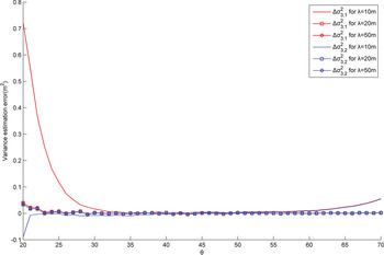
The variance estimation errors for the z coordinate component of the least squares solution (Figure 8) are given as follows:

1. (a) $\Delta \sigma _{3,1}^{2} =\hat {\sigma }_{3,1}^{2} -{\mathop{\sigma}\limits^{\frown}}_{3,1}^{2} $ , where $\hat {\sigma }_{3,1}^{2} $ is the traditional variance estimation, and ${\mathop{\sigma}\limits^{\frown}}_{3,1}^{2} $ is the variance estimated by Equation (19) from the Monte Carlo method;

2. (b) $\Delta \sigma _{3,2}^{2} ={\mathop{\sigma}\limits^{\frown}}_{3,2}^{2} -{\mathop{\sigma}\limits^{\frown}} _{3,1}^{2} $ , where ${\mathop{\sigma}\limits^{\frown}}_{3,2}^{2} $ is the variance estimation by the proposed iterative procedure in Section 3, and ${\mathop{\sigma}\limits^{\frown}}_{3,1}^{2} $ is the variance estimated by Equation (19) based on the Monte Carlo method.

Figure 8.

Variance estimations for the z coordinate component.

Figure 8 shows that the proposed variance estimation ${\mathop{\sigma}\limits^{\frown}}_{3,2}^{2}$ is in better agreement with the variance estimation ${\mathop{\sigma}\limits^{\frown}}_{3,1}^{2} $ based on the Monte Carlo method, especially for relatively short-distance cases and ill-conditioned cases.

4.2. Real underwater positioning

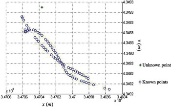
The following positioning scenario is from a real underwater positioning experiment implemented over the Bohai sea area of China. As shown in Figure 9, there are a series of shipborne GNSS kinematic points distributed on the sea level and the positioning precision can achieve a centimetre-level by applying the GNSS post data processing. The distances from the GNSS control points to the known point are measured by the sonar signal where the sonar ranging can achieve decimetre-level precision.

Figure 9.

Positioning configuration under the Gaussian projection coordinate system.

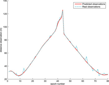
Eighty observations were obtained in the experiment where 16 gross observations are detected by the robust least squares, including the observations at the 7th, 13th,…, 72th, 73th and 77th epoch as shown in Figure 10.

Figure 10.

Distance observations.

By using the 64 normal observations we can obtain the least squares solution

(51) $${{\hat{{\bf x}}}}^G=[4349315.51 \quad 347035.85 \quad 4.02]^{\rm T}$$

of which the posterior variance estimation is

(52) $${\bf D}_{\hat{\bf x}^G} =\left[\matrix{ -0.20 & -0.15 & -1.24 \cr -0.15 &-0.13 & -0.99 \cr -1.24 &-0.99 & -8.06} \right]$$

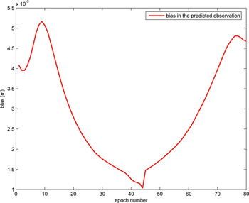
According to the variance matrix Equation (52), we know that the precision of the height coordinate is relatively low because the known points are approximately coplanar and the depth of the unknown point is only about 4 m. By Equation (37) we can then obtain the biases in the predicted distances and they are given in Figure 11. This shows that the bias is inversely proportional to the distance of the observations where the biggest bias 0.165 m happens at the ninth epoch corresponding to the distance observation 24.61 m.

Figure 11.

Biases in predicted distances.

By using the bias estimation for the predicted distances, with Equation (44) and the variance matrix Equation (52) we can then obtain the bias in the location estimation Equation (51) as follows

(53) $${\bf \Delta}^G = \left[\matrix{0.0011 &{-}0.0010 &-1.0499} \right]$$

Because this problem is slightly ill-conditioned in the height direction and the control points are distributed at sea level such that the positional configuration is asymmetrical in the height direction, so the bias in the height direction is larger than those in the x and y directions. This indicates that in ill-conditioned short-distance cases the bias requires particular attention, such as in underwater positioning as well as in mobile positioning.