2. Stellar activity

In the introduction, we asserted that, all else being equal (i.e. at fixed stellar mass and rotation), more metal-rich stars should be more magnetically active. A number of studies have empirically demonstrated this to be the case in recent years. The first we will discuss is the study of See et al. (Reference See, Roquette, Amard and Matt2021). In this work, we studied the activity levels of stars in the Kepler field using the photometric variability amplitude as our magnetic activity proxy (McQuillan et al. Reference McQuillan, Mazeh and Aigrain2014). We found that, broadly speaking, more metal-rich stars do indeed have larger variability amplitudes, indicating that the theoretical expectation outlined in the introduction is correct. It is worth briefly noting that there are a few areas in the mass-period parameter space where this trend does not seem to hold. This is likely to be because the photometric variability amplitude is a less direct tracer of magnetic activity than other activity proxies (see e.g. Reinhold et al. Reference Reinhold, Bell, Kuszlewicz, Hekker and Shapiro2019).

Further evidence that more metal-rich stars are more magnetically active came in the study of See et al. (Reference See, Roquette, Amard and Matt2023). In this work, we once again studied stars in the Kepler field. However, for this study, we used flaring activity as our activity proxy. Specifically, we analysed the normalised flaring luminosity, $R_{\rm flare} = L_{\rm flare}/L_{\rm bol}$ , which is defined as the flare luminosity of a star divided by its bolometric luminosity (Yang and Liu Reference Yang and Liu2019). We fit a power law to our stellar sample of the form

(1) \begin{equation}\log R_{\rm flare} = a\log M_\star + b\log P_{\rm rot} + c{\rm [Fe/H]} + d,\end{equation}

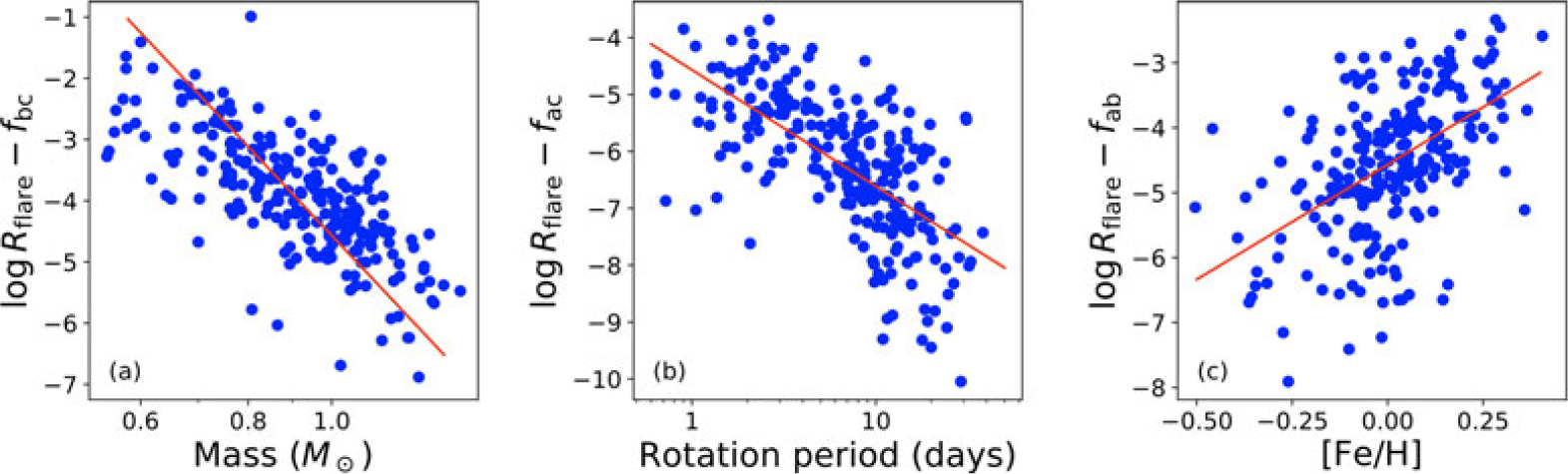
where $M_\star$ is the stellar mass, $P_{\rm rot}$ is the stellar rotation period, and $\rm [Fe/H]$ is the stellar iron abundance. We found the best fit values of $a=-14.95\pm1.36$ , $b=-2.05\pm0.19$ , $c=3.54\pm0.49$ , and $d=-4.57\pm0.14$ . The positive value of the coefficient c on the metallicity term indicates that more metal-rich stars are more active in flares, which, again, is in line with the theoretical expectation outlined in the introduction. Figure 1 shows the mass, period, and metallicity dependence of the normalized flaring luminosity for the stellar sample we considered. In this figure, the f terms on the y axes are the terms from equation (1) not being considered on the x axis. For example, in the left panel, stellar mass is being considered on the x axis and so $f_{bc} = b\log P_{\rm rot} + c{\rm [Fe/H]}$ . The metallicity dependence of stellar flaring can be clearly seen in the right panel of figure 1.

Figure 1.

Normalised flare luminosity vs stellar mass, rotation period and [Fe/H] for a sample of stars in the Kepler field from See et al. (Reference See, Roquette, Amard and Matt2023). For each panel, the f terms on the y axis are the terms from equation (1) not being considered on the x axis. For example, in the left panel, stellar mass is being considered on the x axis and so $f_{bc} = b\log P_{\rm rot} + c{\rm [Fe/H]}$ . The solid lines in each panel are the best fit lines given by equation (1).

Figure 1 Long description

Three scatter plots show the relationship between normalized flare luminosity and different stellar properties. Panel A: The scatter plot shows the relationship between normalized flare luminosity and stellar mass. The x-axis is labeled 'Mass (M☉)' and the y-axis is labeled 'log R_flare - f_bc'. The data points are scattered with a downward trend, and a red line represents the best fit. Panel B: The scatter plot shows the relationship between normalized flare luminosity and rotation period. The x-axis is labeled 'Rotation period (days)' and the y-axis is labeled 'log R_flare - f_ac'. The data points are scattered with a downward trend, and a red line represents the best fit. Panel C: The scatter plot shows the relationship between normalized flare luminosity and [Fe/H]. The x-axis is labeled '[Fe/H]' and the y-axis is labeled 'log R_flare - f_ab'. The data points are scattered with an upward trend, and a red line represents the best fit.

3. Stellar rotation evolution

As discussed in section 2, more metal-rich stars are more magnetically active at a fixed stellar mass and rotation period. How does this affect the long term evolution of stars, in particular, their rotation evolution? Numerical modeling suggests that, at a given age, more metal-rich stars should be rotating more slowly at late ages (Amard and Matt Reference Amard and Matt2020). The physical reason for this is that stellar winds, which are responsible for rotation spin-down on the main sequence, are a magnetically driven phenomenon. As such, more metal-rich stars are expected to have stronger winds, resulting in greater angular momentum-loss and slower rotation at later ages.

A number of observational studies back this up. The first is the study conducted by Amard et al. (Reference Amard, Roquette and Matt2020) who considered the rotation periods of stars in the Kepler field. These authors found that more metal-rich stars were, indeed, rotating more slowly, on average, than metal-poor stars. While not conclusive proof, this was strong evidence that angular momentum-loss via winds is a metallicity dependent process. In a subsequent study, See et al. (Reference See, Lu, Amard and Roquette2024) calculated the ages of these stars using the gyro-kinematic age dating technique (Lu et al. Reference Lu, Angus, Curtis, David and Kiman2021). In that work, we confirmed the expectation that angular momentum-loss from stellar winds is metallicity dependent, with more metal-rich stars spinning slower on average at late ages.

4. Exoplanet evolution

Stellar magnetic activity plays a significant role in the evolution of exoplanets and their atmospheres. One key example is the photoevaporation of planetary atmospheres by high energy stellar radiation, such as X-ray or extreme ultraviolet radiation (together referred to as XUV; Johnstone et al. Reference Johnstone, Güdel, Stökl, Lammer, Tu, Kislyakova, Lüftinger, Odert, Erkaev and Dorfi2015). Given the discussion in sections 2 and 3, an obvious question is how the metallicity of the host-star impacts the photoevaporation of exoplanetary atmospheres? This is the question that we tackled in See et al. (Reference See, Fairman, Amard and Hall2025) using numerical evolution models. This question is complex, with numerous places where the metallicity of the host star plays a role, which we cover here in turn.

The first consideration is how does magnetic activity evolve over time and how does this evolution depend on metallicity? As discussed in section 2, more metal-rich stars are more magnetically active for a given stellar mass and rotation period. However, as discussed in section 3, more metal-rich stars also spin down to slower rotation at late ages and slow rotation is associated with weaker activity (e.g. Noyes et al. Reference Noyes, Hartmann, Baliunas, Duncan and Vaughan1984). A priori, it is unclear which of these effects is larger and, therefore, whether metal-rich stars are more or less magnetically active than metal-poor stars at a given age. The Numerical modeling we conducted in See et al. (Reference See, Fairman, Amard and Hall2025) suggests that it is the former effect that wins out and that metal-rich stars are more magnetically active at late ages even though they are rotating slower than more metal-poor stars.

The second consideration is, what do we exactly mean by a star’s magnetic activity level? When parameterising magnetic activity as a function of Rossby number, it is common to normalise the activity proxy by a star’s bolometric luminosity. For example, when studying X-ray emission, the normalised X-ray luminosity, $R_{\rm X} = L_{\rm X}/L_{\rm bol}$ , is commonly used (Wright et al. Reference Wright, Drake, Mamajek and Henry2011). Without this normalisation, activity-rotation relations have significantly more scatter. However, in the context of photoevaoration of exoplanet atmospheres, the relevant parameter is the X-ray flux received by the planet which depends on the X-ray luminosity, $L_{\rm X}$ , not the normalised X-ray luminosity, $R_{\rm X}$ . It is, therefore, important to realise that another metallicity dependence is introduced when converting from normalised X-ray luminosity to absolute X-ray luminosity since a star’s bolometric luminosity is also metallicity dependent (more metal-rich stars are less luminous; Amard et al. Reference Amard, Palacios, Charbonnel, Gallet, Georgy, Lagarde and Siess2019; See et al. Reference See, Fairman, Amard and Hall2025).

The third consideration is what is the orbital distance of the exoplanet? This parameter is crucial, as it determines how much of the star’s XUV radiation is received by the planet. Our goal in See et al. (Reference See, Fairman, Amard and Hall2025) was to study atmospheric mass-loss in the context of habitability. As such, we modeled exoplanets in the habitable zones of their host stars using the prescription of Kopparapu et al. (2014) to determine the location of the habitable zone. This prescription depends on both the stellar effective temperature and luminosity, which are both dependent on a star’s metallicity. The net effect is that more metal-rich stars have habitable zones at smaller orbital radii (Gallet et al. Reference Gallet, Charbonnel, Amard, Brun, Palacios and Mathis2017; See et al. Reference See, Fairman, Amard and Hall2025).

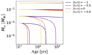
After all of these considerations, what does the atmospheric evolution of exoplanets look like, and what is the metallicity dependence of that evolution? Figure 2 (adapted from See et al. Reference See, Fairman, Amard and Hall2025) shows the predicted atmospheric mass evolution for Earth mass planets orbiting in the habitable zones of solar mass stars. For the planets, initial atmospheric mass fractions of $10^{-1}$ , $10^{-2}$ , $10^{-3}$ and $10^{-4}$ are considered while [Fe/H] values of -1, -0.5, 0 and +0.5 are considered for the host star. Ultimately, we can see that, for a given initial planetary mass fraction, the planets orbiting more metal-rich stars lose their atmospheres quicker than those around metal-poor stars.

Figure 2.

Modeled atmospheric evolution of Earth mass exoplanets orbiting in the habitable zones of solar mass stars. Each track represents the evolution of the planet’s atmospheric mass as it is photoevaporated away by the XUV radiation of its host star. Initial atmospheric mass fractions of $10^{-1}$ , $10^{-2}$ , $10^{-3}$ and $10^{-4}$ are considered for the planet while metallicities of -1, -0.5, 0 and +0.5 are considered for the host star. Figure adapted from See et al. (Reference See, Fairman, Amard and Hall2025).

5. Summary

In recent years, a number of studies have been published looking at how stellar metallicity affects the evolution of stellar activity and rotation as well as the knock on effects for exoplanet evolution. In this contribution, we have discussed these works which we briefly summarise here. All else being equal, more metal-rich stars appear to be more magnetically active. This has been demonstrated by looking at the photometric variability amplitude (See et al. Reference See, Roquette, Amard and Matt2021) and flaring activity (See et al. Reference See, Roquette, Amard and Matt2023) of stars in the Kepler field. It seems likely that all forms of magnetic activity should follow this trend although this has yet to be confirmed. A consequence of increased magnetic activity of metal-rich stars is that they spin down to slower rotation at late ages (Amard and Matt Reference Amard and Matt2020; Amard et al. Reference Amard, Roquette and Matt2020; See et al. Reference See, Lu, Amard and Roquette2024). Finally, recent modeling work suggests that planets in the habitable zones of more metal-rich stars lose their atmospheres to photoevaporation quicker than planets around metal-poor stars See et al. (Reference See, Fairman, Amard and Hall2025).