3.1. Overview and transitions

The data presented in this section relates only to Boger fluids with particle loading. A sample transition sequence for $\phi =0.1$ is presented in figure 3, where figure 3(a) is the flow map ($Re$-space diagram) for $\phi =0.1$ during a RU experiment, figure 3(b) is the corresponding frequency map, and figure 3(c) and figure 3(d) are flow maps from STS experiments performed at $Re=133$ and $Re=200$, respectively. Figure 3(e) shows frequency spectra extracted from figure 3(b) and corresponding to flow states described in figure 3(c) and figure 3(d). Finally, figure 3(f) and figure 3(g) display flow and frequency maps corresponding to figure 3(a) and figure 3(b) but for a RD experiment. A visual difference in flow transitions between RU and RD can be noted, and will be discussed later.

Figure 3.

Example of RU (a,b), STS (c,d) and RD experiments (f,g) for a $\phi =0.1$ fluid (false colours). Panels (a,f) are $Re$-space diagrams (flow maps), (b,g) are frequency maps, (c,d) are space–time diagrams at fixed $Re$ and (e) shows temporal spectra extracted from the (b) frequency map at $Re$ corresponding to (c) and (d). Horizontal dashed lines in (b) and (g), and vertical dashed lines in (e) denote elastic wave frequencies $f^k=k\times f_e$ with $k=[\frac {1}{3},\frac {2}{3}]$ and $k=[\frac {1}{2},1]$ for the two first peaks in RU (b,e) and RD (g), respectively. Here, z is the location along the vertical axis and $f_{max}$ the maximum inner cylinder rotation frequency.

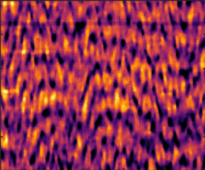
In CF, the space–time diagrams figure 3(a,f) are homogeneous, with all flakes oriented in the azimuthal direction. When TVF arises, the flakes’ orientation in relation to Taylor vortices gives rise to a banded structure. The CF (or TVF) are steady in time and not associated with any characteristic frequencies on the frequency map (figure 3b,g), other than the inner cylinder rotation frequency, that are captured by the method. The end of CF is identified from the flow maps when spatial structures appear.

In the rotating spiral waves (RSW) regime, a base TVF structure is visible, but additional patterns appear due to axial non-axisymmetric elastic waves spiralling either upward or downward (Lacassagne et al. Reference Lacassagne, Cagney, Gillissen and Balabani2020) (figure 3a,c,f). This results in additional and distinct ridges on the frequency maps (figure 3b,g) that do not depend on $Re$, from the onset of which the critical $Re$ for transition from/to RSW can be detected. The existence of TVF (that can be quite difficult to capture, see figure 3a) thus spans from the appearance of spatial structures to the appearance of these ridges. They correspond to the temporal frequencies of RSW, i.e of the primary elastic instability, and their frequency scales as $f^k=k\times f_e$ with $f_e=2c_e/\lambda$ the elastic frequency, $\lambda \simeq d$ a spatial wavelength, and $c_e=\sqrt {\mu /(\rho t_e)}$ the elastic wave celerity. The two first $f^k$ frequencies are illustrated by horizontal dashed lines in figure 3(b) and 3(g). Vertical dashed lines in figure 3(e) for $Re=133$ denote the peaks corresponding to horizontal lines in figure 3(b). The related $k$ values are reported in the figure caption.

Finally, in the EIT domain (EIT), the random alignment of flakes with a set of various spatial flow structures translates into an increasingly chaotic intensity signal and space–time plot (figure 3a,d,f). The distinct peaks in the frequency maps that were present in RSW gradually merge into continuous spectra (figure 3b,g,e). The EIT thus consists in the appearance of spatial and temporal chaos on top of the organised TVF structure, through RSW and the multiplication of vortex merging and splitting events. Critical $Re$ for RSW$\leftrightarrow$EIT transitions are identified from the frequency maps (figure 3b,g), when secondary RSW peaks can no longer be distinguished. Note that some of the spectral signature of RSW may persist into the EIT regime in the form of a consistent smoother peak (see figure 3g, $Re > 170$).

In RD experiments, an additional flow state is encountered in the form of upward spiralling vortices, and labelled SVF for spiral vortex flow (see figure 3f). A summary of critical $Re$ for transitions, $Re_c$, is provided in figure 4(a,b) for RU and RD experiments, respectively. The experiments were repeated at least four times (see table 1) and excellent consistency on the succession of flow states was encountered. The reported visualisations correspond to single experimental runs, but critical $Re$ values are averaged over all repeats, and the standard deviations over critical $Re$ provide error bars for figure 4.

Figure 4.

Critical $Re$–$\phi$ maps for transitions to TVF, RSW, EIT and SVF in RU (a) and RD (b) experiments. Hysteretic behaviours are illustrated for transitions to/from EIT, RSW and TVF in panels (ci, cii and ciii), respectively (triangles pointing upwards for RU, downwards for RD).

It can be seen that the addition of particles initially decreases the critical $Re$ for the CF$\longrightarrow$TVF transition at the lowest particle volume fraction, but as $\phi$ is increased above 0.01, the critical $Re$ increases, stabilising the flow. The same trend is observed in figure 4(b) for the RD experiments for $\phi <0.1$. Note that in Newtonian suspensions, the addition of particles in the same volume fraction range mostly leads to a minor destabilisation of the CF with respect to TVF (Majji et al. Reference Majji, Banerjee and Morris2018; Gillissen & Wilson Reference Gillissen and Wilson2019; Ramesh et al. Reference Ramesh, Bharadwaj and Alam2019). The opposite trend observed here must therefore be attributed to the combination of particles and viscoelastic fluid matrix; while both properties in isolation tend to destabilise CF compared with the Newtonian case, they have the opposite effect when combined.

For the $\phi =0.1$ RD experiments, SVF is observed at $Re$ values much lower than the critical $Re$ for CF$\longrightarrow$TVF transition in RU. This new state is illustrated in the flow map and corresponding frequency map of figure 5. It appears to coexist with RSW in the $Re$ range from 120 to 140 (figure 5a, close-up in figure 5b). We also note that SVF is not associated with any spectral signature on its own: the frequency map in the $Re$ range of 20–120 is similar to that expected for TVF (figure 5c). Such spiralling behaviour was previously reported in particle suspensions in Newtonian fluids in RD (Majji et al. Reference Majji, Banerjee and Morris2018) but also RU (Ramesh et al. Reference Ramesh, Bharadwaj and Alam2019; Ramesh & Alam Reference Ramesh and Alam2020), sometimes interpenetrating or coexisting with other flow states (Majji et al. Reference Majji, Banerjee and Morris2018; Ramesh & Alam Reference Ramesh and Alam2020). The fact that the new state is found only in RD tests suggests a modification of the nature of primary instabilities in particle-loaded Boger fluids at non-dilute volume fractions ($\phi \succeq 0.05$). The SVF is unlikely to be caused by buoyancy or particle-migration effects, since it arises when ramping down from chaotic states (EIT–RSW) in which particles are expected to be well mixed by strong axial flow velocity fluctuations. The coexistence of flow states, which was already observed for particles in Newtonian solvents (Ramesh et al. Reference Ramesh, Bharadwaj and Alam2019; Dash et al. Reference Dash, Anantharaman and Poelma2020; Ramesh & Alam Reference Ramesh and Alam2020), is for the first time reported here for particle suspensions in Boger fluids.

Figure 5.

Illustration of the SVF state for RD experiments at $\phi =0.1$, on the flow map (a) and frequency map (c) (focus from figure 3f and 3g). Vertical dotted lines highlight transitions from RSW, RSW$+$SVF, SVF and CF from right to left (decreasing $Re$). A close-up of the flow map in the coexisting state range RSW$+$SVF is provided in panel (b) ($Re$ axis ranging from 118 to 136, $z/d$ axis from 5 to 20).

The higher order transition to RSW (figure 4a,b) arises very soon after the onset of TVF (Lacassagne et al. Reference Lacassagne, Cagney, Gillissen and Balabani2020). After a slight destabilisation at $\phi =0.01$, a stabilising effect by particle addition is again reported, with critical $Re$ values increasing with $\phi$. The RD results in figure 4(b) follow the same trend. Averaging on all experiments, TVF has a very narrow $Re$ range of existence ${\rm \Delta} Re_{TVF}\sim 1$ with yet ${\rm \Delta} t_{TVF}>10\times t_e$. It is the first in a series of transitions leading to more complex flow states. In some higher $\phi$ cases, TVF can sometimes not be seen clearly (figure 3a) and the primary transition could be either CF$\leftrightarrow$TVF or CF$\leftrightarrow$RSW within the margin of error of this study. The results thus suggest that increasing particle concentration reduces ${\rm \Delta} Re_{TVF}$, promoting CF–RSW as the primary instability upon particle addition. However a precise understanding of this effect calls for a more accurate investigation in the $Re=[100 - 120]$ range.

For the RSW to EIT transition, the trends for critical $Re$ are globally similar to those previously reported for transition to RSW, i.e. a destabilisation by $\phi =0.01$ followed by a stabilisation both in RU and RD cases, upon increased $\phi$. This non-monotonic trend is more pronounced for the RSW$\leftrightarrow$EIT transition compared with those observed for lower order transitions. The combined effects of particles and viscoelasticity, which would have been expected to separately lead to earlier second-order flow transitions, here again appear to delay transition to chaotic patterns.

3.2. Effect of particle loading on RSW and EIT properties

The effects of particle loading on EIT features can be characterised using spatio-temporal flow properties at a constant Reynolds number. Figure 6 shows two dimensional FFTs in time and space of STS experiments. Peaks of such spectra correspond to dominant time and length scales of the flow. The RSW is described by a set of discrete and identifiable peaks in space but also in time (see for example figure 6c). On the other hand, EIT displays a broadband behaviour characteristic of a turbulent state, with no distinct peak (see e.g. figure 6b). The temporal spectra projected on upper-right parts allow to distinguish between RSW (clear temporal peak, figure 6c) and EIT (no clear temporal peak, figure 6a,b,d). Figure 6 shows that the collapse of RSW spectra into broadband EIT, which occurs as $Re$ is increased, is delayed by the increase in $\phi$. In the $\phi =0.01$ case (top line) $Re=167$ (figure 6b) already corresponds to a turbulent signature without peaks, while for $\phi =0.1$ (bottom line), peaks are still visible at $Re=200$ (figure 6d), although they are less distinct than at $Re=133$ (figure 6c). In other words, the presence of particles delays the transition to EIT, as previously observed, but also preserves the large-scale spatial structure of RSW into EIT.

Figure 6.

Two dimensional FFTs (time and space) of STS experiments for $\phi =0.01$ (a,b) and $\phi =0.1$ (c,d). Top left and top right parts on each panel display mean spectra in the frequency and space dimensions, respectively. The spatial wavelength axis is scaled by the gap size $d$ and the temporal frequency axis by $1/t_e$.

3.3. Hysteretic behaviour

At $\phi =0$, critical $Re$ for CF–TVF and TVF–RSW transitions are higher for RU experiments than for RD experiments (see figure 4cii,ciii). This is the signature of a (moderately) subcritical bifurcation (Martínez-Arias & Peixinho Reference Martínez-Arias and Peixinho2017). Particle addition reverses the hysteresis; even at the lower $\phi$ values, the critical $Re$ values in RD experiments become larger than those found in RU tests, for both transitions. The flow transitions back to lower order states at higher $Re$ that are seen in the RU tests, and the difference in critical $Re$ values due to this reversed hysteretic behaviour, increases with the order of the transition (larger for RSW–EIT transition than for CF–TVF transition), and with increasing $\phi$.

The origin of such a reversed hysteretic behaviour may, at first, be attributed to elastic or inertial particle migration. Indeed, particles migrating away from the inner cylinder in CF during RU tests would induce lower inner viscosity and higher $Re$, leading to a lower apparent critical $Re$ in RU compared with the RD case where particles are expected to be evenly dispersed and the viscosity homogeneous. This is in qualitative agreement with a similar reverse hysteresis observed by Ramesh et al. (Reference Ramesh, Bharadwaj and Alam2019) for the CF–TVF primary transition in Newtonian particle suspensions, suggesting that inertial migration may play a role. Moreover, the shortest time scale at which elastic migration effects would arise, estimated according to the modelling of D'Avino, Greco & Maffettone (Reference D'Avino, Greco and Maffettone2017), is found to be $\sim 50$ s, comparable to and even shorter than the typical times particles spent in CF during a RU experimental protocol. Thus, elastic migration may also be at play when considering primary instabilities.

However, a stronger reversed hysteresis is observed for higher order RSW$\leftrightarrow$EIT transition, for which particles are expected to be well mixed in both states, which suggests that migration alone cannot explain the observed hysteretic phenomena. This new and striking result suggests that the particles act on elasto-inertial patterns with mechanisms other than migration, and more importantly that this action corresponds to a damping or attenuation of elasto-inertial features. Recent findings on local stress concentration and elastic thickening (see e.g. Yang & Shaqfeh Reference Yang and Shaqfeh2018a,Reference Yang and Shaqfehb) in particles suspended in viscoelastic media might further explain this macroscopic behaviour.