MONOTONICITY RESULTS FOR SINGLE-SERVER FINITE-CAPACITY QUEUES WITH RESPECT TO DIRECTIONALLY CONVEX ORDER

Shigeo Shioda; Daisuke Ishii

doi:10.1017/S026996480418306X

MONOTONICITY RESULTS FOR SINGLE-SERVER FINITE-CAPACITY QUEUES WITH RESPECT TO DIRECTIONALLY CONVEX ORDER

Published online by Cambridge University Press: 01 July 2004

Shigeo Shioda and

Daisuke Ishii

Show author details

Shigeo Shioda: Affiliation:
Urban Environment Systems, Faculty of Engineering, Chiba University, 1-33 Yayoi, Inage, Chiba 263-8522, Japan, E-mail: shioda@faculty.chiba-u.jp
Daisuke Ishii: Affiliation:
Urban Environment Systems, Faculty of Engineering, Chiba University, 1-33 Yayoi, Inage, Chiba 263-8522, Japan, E-mail: shioda@faculty.chiba-u.jp

Article contents

Abstract
1. INTRODUCTION
2. PRELIMINARIES
3. COMPARISON RESULTS FOR QUEUES WITH DIFFERENT WORK PROCESSES
4. COMPARISON RESULTS FOR QUEUES WITH DIFFERENT INTERARRIVAL PROCESSES
5. UPPER BOUND OF WORK-LOSS PROBABILITY
6. NUMERICAL EXAMPLES
7. CONCLUDING REMARK
Acknowledgment
References

Rights & Permissions

Abstract

In this article, we investigate single-server finite-capacity queues where the partial acceptance rule is applied. In particular, we focus on the monotonicity of the amount of lost (processed) work in the queues with respect to the directionally convex order of work or interarrival processes. We first compare the queues that differ only in their work processes and show that if the work processes are directionally convex ordered, so is the amount of work lost (or processed) in the systems. Next, we compare the queues that differ only in their interarrival processes and show that if the interarrival processes are directionally convex ordered, so is the amount of work lost (or processed) in the systems. Using these results, we establish the formula that gives the upper bound of work-loss probability based only on the marginal distributions of work and interarrival processes. Numerical experiments using the data of actual-LAN (local area network) traffic show that the derived formula gives tight bounds sufficient for practical use.

Information

Type: Research Article
Information: Probability in the Engineering and Informational Sciences , Volume 18 , Issue 3 , July 2004 , pp. 369 - 393

DOI: https://doi.org/10.1017/S026996480418306X [Opens in a new window]
Copyright: © 2004 Cambridge University Press

1. INTRODUCTION

In this article, we consider a single-server finite-capacity queue that has the following properties. In the time interval (0,∞), customers arrive at the queue. The nth customer arrives at T_n and brings the work of size X_n (say, in bytes). The customers are allowed to arrive in a group; hence, T_n might be equal to T_n+1 for n ≥ 1. The queuing system has limited buffer space of size B. If unoccupied buffer space is greater than X_n upon the arrival of the nth customer, the whole work brought by the nth customer is accepted. Otherwise, a part of the work whose amount is equal to the unoccupied buffer space is accepted and the rest of the work is lost (partial acceptance rule). The accepted work is stored in the buffer and the work in the buffer is continuously processed at a constant rate C.

The above-mentioned queue is equivalent to a fluid queue with batch fluid inputs; batch fluid inputs mean that a batch of fluid sequentially arrives at random times. Gani and Prabu [3,4] found the limiting distribution of the amount of work in the queue where a customer (a batch of fluid) sequentially arrives in accordance with a Poisson process. Takács [12] also studied such a queue where customers arrive in accordance with a Poisson process and the size of work of each customer depends on the level of buffer occupation. Takada and Miyazawa [13,14] studied a fluid queue with continuous fluid and batch fluid inputs where both inputs are governed by a finite-state Markov chain. Under the general work process X = (X₁,X₂,…) and arrival process T = (T₁,T₂,…), however, the performance of the above-mentioned queue is analytically untractable. This article investigates the qualitative properties of the above-mentioned queue under general work and arrival processes. In particular, we focus on the monotonicity of the amount of lost (processed) work with respect to the strength of autocorrelation of work and arrival processes. For example, for two queuing systems where the first has a less correlated arrival process than the second, we would like to show that the amount of lost work of the first queue is stochastically smaller than the second.

We obtain the comparison results by exploiting the notion of directionally convex ordering. The directionally convex ordering is a useful tool for comparing the strength of autocorrelation of stochastic processes and has been used for the proof of Ross's conjecture (see Chang, Chao, and Pinedo [1] and Meester and Shanthikumar [7]). It has also been used for obtaining the monotonicity of the performance of batch-arrival queues with respect to batch sizes (see Chang, Chao, Pinedo, and Shanthikumar [2] and Meester and Shanthikumar [7]). For other applications of directionally convex order to queuing analysis, see Toyoizumi, Shanthikumar, and Wolff [15].

To state the main result, let us define

; in this article, the stochastic process U = (U₁,U₂,…) is referred to as the interarrival process. We first compare the queues that differ only in their work processes and show that if the work processes are directionally convex ordered, so is the amount of work lost in the systems. Next, we compare the queues that differ only in their interarrival processes and show that if the interarrival processes are directionally convex ordered, so is the amount of work lost in the systems. Using these results, we establish the formula that gives the upper bound of work-loss probability based only on the marginal distributions of work and interarrival processes.

The result of this article would have a wide range of applications. Let us consider a packet-handling procedure of a router in the Internet. When the router receives a packet, it looks into the header of the packet and finds its next hop via the routing table. Then, the packet is stored in the buffer and sent to the next hop in a first-in first-out discipline. As it stands, this packet-handling process can be modeled by a single-server queue. Thus, if we had all of the information about the input process (e.g., the arrival times and the lengths of all packets), then we could evaluate the amount of lost work in the router. Because of the limitation of traffic measurement, however, we cannot precisely know the amount of input traffic in a fine timescale. The measurement interval of the amount of traffic is at least one second or a few seconds. If we assume the model where customers arrive in batch at the beginning of every measurement interval, we can apply the result of this article to evaluate the work-loss probability of the queue even in such a case. Our model does not precisely represent the actual packet-handling procedure because the partial acceptance of the packet is not allowed in actual situations, whereas it is allowed in our model. The modeling error, however, would not cause a serious estimation error because the packet size is becoming much smaller than the size of buffer due to the recent exponential growth in the capacity of routers in the Internet.

A considerable number of studies have been made on the effects of the variation and autocorrelation of the input process on the performance of queues. For example, the effects of batch size variation on the performance of the queue were investigated in Miyazawa and Shanthikumar [8], Jean-Marie and Liu [6], Chang et al. [2], and Shanthikumar [10]. Miyazawa and Shanthikumar [8] studied the monotonicity of loss probabilities of the M^[X]/GI/1/N and GI/M^[X]/1/N queues with respect to the batch size of arrival and service processes. Jean-Marie and Liu [6] obtained a lower bound (in the increasing convex order sense) for the response time of the GI^[X]/GI/1 queue. Chang et al. [2] showed that the amounts of lost (and accepted) work in G^[X]/M(n)/1/N → /M(n)/1/N → ··· → /M(n)/1/N queues are stochastically ordered when their batch-size processes are ordered in the sense of directionally convex ordering. Shanthikumar [10] showed that the number of jobs, workload, and the waiting time of bulk arrival queues are stochastic increasing convex with respect to the bulk size. The effects of service-time variation on the performance of the queue were investigated in Chang et al. [1] and Meester and Shanthikumar [7]. Many interesting results on the stochastic comparison of queuing systems are well explained in Shaked and Shanthikumar [9] and Stoyan [11].

The article is organized as follows. In Section 2, we explain several notions of stochastic orderings for random variables and stochastic processes, including directionally convex ordering. In Section 3, we show that if the work processes are directionally convex ordered, so is the amount of work lost and accepted in the systems. In Section 4, we compare the queues that differ only in the interarrival process and show that if the interarrival processes are directionally convex ordered, so is the amount of work lost in the systems. In Section 5, among work (interarrival) processes that have a given marginal distribution, we identify the worst work (interarrival) process in terms of directionally convex ordering and derive the bound of work-loss probability in a form that is explicitly computable. In Section 6, we evaluate the tightness of the derived bound through numerical experiments. In Section 7, we make some remarks about the results.

2. PRELIMINARIES

In this section, we show the definitions and related results of several stochastic orderings. For the details, see Chang et al. [1] or Meester and Shanthikumar [7].

2.1. Directional Convexity

Let ≤ denote coordinatewise ordering for real vectors: For x = (x₁,…,x_m) and y = (y₁,…,y_m), x ≤ y if x_i ≤ y_i, for i = 1,…,m. We use [x, z] ≤ y as a shorthand for x ≤ y and z ≤ y. Similarly, we use as a shorthand y ≤ [x, z] for y ≤ x and y ≤ z.

Definition 2.1: A function

is directionally convex (concave) if for any

, such that x⁽¹⁾ ≤ [x⁽²⁾, x⁽³⁾] ≤ x⁽⁴⁾ and x⁽¹⁾ + x⁽⁴⁾ = x⁽²⁾ + x⁽³⁾,

We denote this by f ∈ dcx (dcv). If, in addition, f is increasing, then we write f ∈ idcx (idcv). Similarly, if f is decreasing, then we write f ∈ ddcx (ddcv). Moreover, a function

is directionally convex (concave) if each of the coordinate functions g_i(x),i = 1,…,n, defined by g(x) = (g₁(x),…,g_n(x)), is directionally convex (concave).

Lemma 2.2: Suppose

. If f,g ∈ idcx (idcv), then

. In particular, if

is increasing and convex, then

Lemma 2.3: Suppose

. If f ∈ ddcx (ddcv) and g ∈ idcx (idcv), then

. Similarly, if f ∈ idcx (idcv) and g ∈ ddcx (ddcv), then

2.2. Directionally Convex Ordering

Definition 2.4: Let X and Y be random variables in

. Then, X is said to be smaller than Y in the sense of increasing convex (concave) ordering if E [f (X)] ≤ E [f (Y)] for any increasing and convex function f. We write this as X ≤_icx (≤_icv)Y.

Definition 2.5: Let X and Y be random variables in

. Then, X is said to be smaller than Y in the sense of directionally convex (concave) ordering if E [f (X)] ≤ E [f (Y)] for all

. We write this as X ≤_dcx (≤_dcv)Y.

Definition 2.6: Let {X(t),t ≥ 0} and {Y(t),t ≥ 0} be continuous-time stochastic processes. Then, {X(t)} is said to be smaller than {Y(t)} in the sense of directionally convex (concave) ordering if for any finite

and any 0 ≤ t₁ < t₂ < ··· < t_k,

We write this as {X(t)} ≤_dcx {Y(t)}.

Definition 2.7: Let {X_n,n = 1,2,…} and {Y_n,n = 1,2,…} be discrete-time stochastic processes. Then, {X_n} is said to be smaller than {Y_n} in the sense of directionally convex (concave) ordering if for any finite k and any 0 ≤ n₁ < n₂ < ··· < n_k,

We write this as {X_n} ≤_dcx {Y_n}.

The other relations ≤_dcv, ≤_idcx, ≤_idcv, ≤_ddcx, and ≤_ddcv for random vectors and stochastic processes are defined in the same way as in Definitions 2.5, 2.6, and 2.7.

The following lemma is the immediate consequence of Lorentz's inequality (see Chang et al. [1], Meester and Shanthikumar [7], or Toyoizumi et al. [15]).

Lemma 2.8: Let X be a random vector in

, each coordinate of which X_i, i = 1,…,m, has identical marginal distribution F, and le

be a random vector in

, each coordinate of which

, is defined by

where

is the complementary marginal distribution function of X and U is a uniform (0,1) random variable. Then,

3. COMPARISON RESULTS FOR QUEUES WITH DIFFERENT WORK PROCESSES

In this section, we stochastically compare the amount of lost (or processed) work in the queues that differ only in their work processes. We define the following:

1. W(t; X,U): the amount of work in the buffer at t when the work process is X and the interarrival process is U.

2. L(t; X,U): the amount of work lost by buffer overflow during [0,t] when the work process is X and the interarrival process is U.

3. D(t; X,U): the amount of work processed during [0,t] when the work process is X and the interarrival process is U.

In what follows, without loss in generality, we assume W(0−, X,U) = 0. We also define

Lemma 3.1: Let x and u be deterministic work and interarrival processes (using lowercase letters to distinguish the deterministic case). Then, W(t; x,u), L(t; x,u), and D(t; x,u) are increasing functions of x.

Proof: To prove the lemma, it suffices to show that for any x⁽¹⁾ and x⁽²⁾ such that x⁽¹⁾ ≤ x⁽²⁾,

To this end, let us define

First, observe that D₁(T₁) = D₂(T₁) = 0. Moreover, since x₁⁽¹⁾ ≤ x₁⁽²⁾, it follows that

Thus, Eq. (3.2) holds at t = T₁. Now, let us suppose that Eq. (3.2) holds at t = T_n; that is,

It follows from Eq. (3.5) that for t ∈ (T_n,T_n+1),

Moreover, since W₁(T_n+1−) < W₂(T_n+1−) and L₁(T_n+1−) < L₂(T_n+1−), which we have just proved, it follows from x_n+1⁽¹⁾ ≤ x_n+1⁽²⁾ that

Similarly, it follows that for t ∈ (T_n,T_n+1] ,

Hence, Eq. (3.2) holds for t ∈ (T_n,T_n+1) and so the proof is completed by induction. █

Remark 3.2: The intuitive result of Lemma 3.1 does not hold when the whole acceptance rule is applied (i.e., if the unoccupied buffer space is smaller than the size of work brought by a customer, the entire work is lost).

Lemma 3.3: Let x and u be deterministic work and interarrival processes. Then, L(t; x,u) and D(t; x,u) are respectively directionally convex and directionally concave in x.

Proof: We first show that L(t; x,u) and W(t; x,u) + L(t; x,u) are directionally convex in x. To this end, it suffices to show that for any x⁽ⁱ⁾,i = 1,…,4, such that x⁽¹⁾ + x⁽⁴⁾ = x⁽²⁾ + x⁽³⁾ and x⁽¹⁾ ≤ [x⁽²⁾, x⁽³⁾] ≤ x⁽⁴⁾,

Let us define

Since [x − B]⁺ is convex in x, it follows that

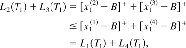
and thus Eq. (3.9) holds at t = T₁. Moreover, since W_i(T₁) + L_i(T₁) = W_i(T₁−) + L_i(T₁−) + x₁⁽ⁱ⁾ = x₁⁽ⁱ⁾,i = 1,…,4, it follows from x₁⁽²⁾ + x₁⁽³⁾ = x₁⁽¹⁾ + x₁⁽⁴⁾ that

and thus Eq. (3.10) also holds at t = T₁. Next, let us suppose that Eqs. (3.9) and (3.10) hold at t = T_n; that is,

Since no customer arrives and thus no work is lost during (T_n,T_n+1), it follows from Eq. (3.14) that Eq. (3.9) holds for t ∈ (T_n,T_n+1). To prove Eq. (3.10) for t ∈ (T_n,T_n+1), we consider the following six cases:

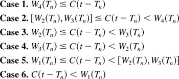
(Note that W₁(T_n) ≤ [W₂(T_n),W₃(T_n)] ≤ W₄(T_n) follows by Lemma 3.1.) For Case 1, observing that W₁(t) = W₂(t) = W₃(t) = W₄(t) = 0, we obtain

where the inequality follows from the fact that Eq. (3.9) holds for t ∈ (T_n,T_n+1), which we have just proved. (In what follows, we repeatedly use this fact.) For Case 2, observing that 0 = W₁(t) = W₂(t) = W₃(t) < W₄(t), we obtain

For Case 3, observing that 0 = W₁(t) = W₂(t) < W₃(t) ≤ W₄(t), we obtain

For Case 4, the desired result follows along the lines of the proof for Case 3. For Case 5, observe that

which yields

For Case 6, since W_i(t) + L_i(t) = W_i(T_n) + L_i(T_n) − C(t − T_n), i = 1,…,4, it follows that

Hence, for all cases, Eq. (3.10) holds. Thus, by induction, Eq. (3.10) holds for t ∈ (T_n,T_n+1).

Next, we show that Eqs. (3.9) and (3.10) hold at t = T_n+1. First, observe that W_i(T_n+1) + L_i(T_n+1) = W_i(T_n+1−) + L_i(T_n+1−) + x_n+1⁽ⁱ⁾ and x_n+1⁽²⁾ + x_n+1⁽³⁾ = x_n+1⁽¹⁾ + x_n+1⁽⁴⁾. Thus, we obtain

and so Eq. (3.9) holds at t = T_n+1. To show Eq. (3.10) at t = T_n+1, we consider the following six cases:

(Note that W₁(T_n+1−) ≤ [W₂(T_n+1−),W₃(T_n+1−)] ≤ W₄(T_n+1−) by Lemma 3.1.) For Case 1, no work is lost at T_n+1 and thus we obtain

For Case 2,

For Case 3,

For Case 4, the desired result follows along the lines of the proof for Case 3. For Case 5,

where the first inequality follows from the fact that Eq. (3.10) holds at t = T_n+1−, which we have proved. For Case 6,

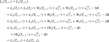
where the first inequality also follows from the fact that Eq. (3.10) holds at t = T_n+1−. Thus, for all cases, Eq. (3.9) holds at t = T_n+1. Finally, by induction, Eqs. (3.9) and (3.10) follow for all t(≥ 0). Now, remember that

Hence, D(t; x,u) is directionally concave in x because W(t; x,u) + L(t; x,u) is directionally convex in x, which we have just proved. █

Theorem 3.4: If X₁ ≤_idcx X₂, then for any u,

Proof: In view of Definitions 2.5 and 2.6, it suffices to check that for any function

, any finite

, and any 0 ≤ t₁ < t₂ < ··· < t_k,

To this end, observe that L(t; x,u) is increasing and directionally convex in x by Lemmas 3.1 and 3.3. Thus, it follows by Lemma 2.2 that

is also increasing and directionally convex. Thus, the proof is completed by the definition of increasing directionally convex ordering. █

Corollary 3.5: If X₁ ≤_idcx X₂, then for any n ≥ 1 and u,

Proof: It suffices to show that for any increasing and convex function

As we have shown in the proof of Lemmas 3.1 and 3.3, L(T_n; x,u) is increasing and directionally convex in x when T_n is fixed. Thus, it follows by Lemma 2.2 that

is also increasing and directionally convex. Hence, it turns out that since X₁ ≤_idcx X₂,

from which Eq. (3.32) follows. █

Theorem 3.6: If X₁ ≤_idcv X₂, then, for any u,

Proof: In view of Definitions 2.5 and 2.6, it suffices to check that for any

and any 0 ≤ t₁ < t₂ < ··· < t_k,

To this end, observe that D(t; x) is increasing and directionally concave in x by Lemmas 3.1 and 3.3. Then, it follows by Lemma 2.2 that

is increasing and directionally concave. Thus, the proof is completed by the definition of increasing directionally concave ordering. █

Corollary 3.7: If X₁ ≤_idcv X₂, then for any n ≥ 1 and any u,

Proof: It suffices to show that for any increasing and concave function

As we have shown in the proof of Lemmas 3.1 and 3.3, D(T_n; x,u) is increasing and directionally concave in x when T_n is fixed. Thus, it follows by Lemma 2.2 that

is also increasing and directionally concave. Hence, it turns out that since X₁ ≤_idcv X₂,

from which Eq. (3.35) follows. █

4. COMPARISON RESULTS FOR QUEUES WITH DIFFERENT INTERARRIVAL PROCESSES

In this section, we stochastically compare the amount of lost (or processed) work in the queues that differ only in their interarrival processes.

Lemma 4.1: Let x be a deterministic work process and let u be an interarrival process. Then, W(T_n; x,u) and L(T_n; x,u) are decreasing functions of u and D(T_n; x,u) is an increasing function of u.

Proof: To prove the lemma, it suffices to show that for any u⁽¹⁾ and u⁽²⁾ such that u⁽¹⁾ ≤ u⁽²⁾,

For notational simplicity, let us define

First, observe that Eq. (4.1) holds for n = 1 because

Next, let us suppose that Eq. (4.1) holds for n = k; that is,

Since u_k⁽¹⁾ ≤ u_k⁽²⁾, it follows from Eq. (4.4) that

and thus Eq. (4.1) holds for n = k + 1. Hence, the proof is completed by induction. █

Lemma 4.2: Let x and u be a deterministic work process and an interarrival process, respectively. Then, L(T_n; x,u) and D(T_n; x,u) are respectively directionally convex and directionally concave in u for all n ≥ 1.

Proof: First, we show that L(T_n; x,u) and W(T_n; x,u) + L(T_n; x,u) are directionally convex in u for all n. To this end, it suffices to show that the following relations hold for all n ≥ 1 and for any x⁽ⁱ⁾,i = 1,…,4, such that x⁽¹⁾ + x⁽⁴⁾ = x⁽²⁾ + x⁽³⁾ and x⁽¹⁾ ≤ [x⁽²⁾, x⁽³⁾] ≤ x⁽⁴⁾:

It is easy to see that Eqs. (4.6) and (4.7) hold for n = 1. Next, let us suppose that Eqs. (4.6) and (4.7) hold for n = k; that is,

To prove that Eqs. (4.6) and (4.7) also hold for n = k + 1, we consider the following six cases:

(Note that by Lemma 4.1, W₄(T_k) − Cu_k⁽⁴⁾ ≤ [W₂(T_k) − Cu_k⁽²⁾,W₃(T_k) − Cu_k⁽³⁾] ≤ W₁(T_k) − Cu_k⁽¹⁾ because u_k⁽¹⁾ ≤ [u_k⁽²⁾,u_k⁽³⁾] ≤ u_k⁽⁴⁾.)

For Case 1, observe that W_i(T_k+1−) = 0, i = 1,…,4, and so

Thus, we obtain

and

For Case 2, observing that W₁(T_k+1−) > W₂(T_k+1−) = W₃(T_k+1−) = W₄(T_k+1−) = 0, we obtain

and

For Case 3, observing that W₁(T_k+1−) ≥ W₂(T_k+1−) > W₃(T_k+1−) = W₄(T_k+1−) = 0, we obtain

and

For Case 4, the desired result follows through an argument similar to that for Case 3. For Case 5, observing that W₁(T_k+1−) ≥ [W₂(T_k+1−),W₃(T_k+1−)] > W₄(T_k+1−) = 0, we obtain

To prove Eq. (4.6) when n = k + 1 for Case 5, we further decompose Case 5 into the following six cases:

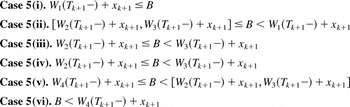
For Cases 5(i) and 5(ii),

For Case 5(iii),

For Case 5(iv), the desired result follows from the argument similar to that for Case 5(iii). For Case 5(v),

For Case 5(vi),

Thus, for Case 5, Eq. (4.6) also holds when n = k + 1. To prove that Eq. (4.7) holds when n = k + 1 for Case 6, observe that W₁(_k+1−) ≥ [W₂(T_k+1−),W₃(T_k+1−)] ≥ W₄(T_k+1−) > 0. Thus, we obtain

and thus Eq. (4.7) holds for n = k + 1. It follows along the lines of the proof for Case 5 that Eq. (4.6) also holds for Case 6 when n = k + 1.

Thus, for all cases, Eqs. (4.6) and (4.7) hold for n = k + 1, and so Eqs. (4.6) and (4.7) hold for all n by induction. Now, remember that

Thus, D(T_n; x,u) is directionally concave in u because W(T_n; x,u) + L(T_n; x,u) is directionally convex in u, which we have just proved. █

Now, define

Note that {L_n(x,U₁),n = 1,2,…} and {D_n(x,U₁),n = 1,2,…} can be regarded as discrete-time stochastic processes.

Theorem 4.3: If U₁ ≤_ddcx U₂, then {L_n(x,U₁),n = 1,2,…} ≤_idcx {L_n(x,U₂), n = 1,2,…} for all x.

Proof: In view of Definitions 2.5 and 2.6, it suffices to check that for any function

and any 0 ≤ n₁ < n₂ < ··· < n_k,

To this end, observe that L(T_n; x,u) is decreasing and directionally convex in u by Lemmas 4.1 and 4.2. Thus, it follows by Lemma 2.2 that

is also decreasing and directionally convex. Thus, the proof is completed by the definition of decreasing directionally convex ordering. █

The next result readily follows from Theorem 4.3.

Corollary 4.4: If U₁ ≤_ddcx U₂, then L(T_n; x,U₁) ≤_icx L(T_n; x,U₂).

Theorem 4.5: If U₁ ≤_idcv U₂, then {D_n(x,U₁),n = 1,2,…} ≤_idcv {D_n(x,U₂), n = 1,2,…} for all x.

Proof: In view of Definitions 2.5 and 2.6, it suffices to check that for any function

and for 0 ≤ n₁ < n₂ < ··· < n_k,

To this end, observe that D(T_n; x,u) is increasing and directionally concave in u by Lemmas 4.1 and 4.2. Thus, it follows from Lemma 2.2 that

is also increasing and directionally concave. Thus, the proof is completed by the definition of increasing directionally concave ordering. █

The following result readily follows from Theorem 4.5.

Corollary 4.6: If U₁ ≤_idcv U₂, then D(T_n; x,U₁) ≤_icv D(T_n; x,U₂) for all x.

5. UPPER BOUND OF WORK-LOSS PROBABILITY

Definition 5.1: We say that X = (X₁,X₂,…) is a stationary work process with the marginal distribution F if each of its coordinates X_i, i = 1,2,…, is identically distributed with distribution function F. We denote this by

. Furthermore, let X^excor(F) = (X₁^excor(F),X₂^excor(F),…) be the stationary work process whose coordinates are defined by

where

is the complementary marginal distribution function of X and U is a uniform (0,1) random variable. We refer to X^excor(F) as an extremal autocorrelated arrival process with marginal distribution F.

Remark 5.2: The notion of stationarity used above is different from (much weaker than) the usual definition of stationarity because the latter requires that (X_n+1,X_n+2,X_n+3,…) has the same joint distribution as that of (X₁,X₂,X₃,…) for all n.

Lemma 5.3: If the work process and interarrival process are independent, then for any

and for any U,

Proof: It follows by Lemma 2.8 that for any

and finite

Then, by Definition 2.7, X ≤_dcx X^excor(F). Hence, by Corollary 3.5,

which yields

A similar discussion leads to E [D(T_n; X,U)] ≥ E [D(T_n; X^excor(F),U)] because X^excor(F) ≤_dcv X. █

Definition 5.4: We say that U = (U₁,U₂,…) is a stationary interarrival process with marginal distribution G if each of its coordinates U_i, i = 1,2,…, is identically distributed with distribution function G. We denote this by

. Furthermore, let U^excor(G) = (U₁^excor(G),U₂^excor(G),…) be the stationary interarrival process whose coordinates are defined by

where

is the complementary marginal distribution function of U and U is a uniform (0,1) random variable. We refer to U^excor(G) as an extremal correlated interarrival process with marginal distribution G.

Lemma 5.5: If the work process and interarrival process are independent from each other, then for any X and for any

Proof: By the same discussion used in the proof of Lemma 5.3, we obtain U ≤_dcx U^excor(G). Thus, by Corollary 4.4,

which yields

A similar discussion leads to E [D(T_n; X,U)] ≥ E [D(T_n; X,U^excor(G))] because U^excor(F) ≤_dcv U. █

The following result readily follows from Lemmas 5.3 and 5.5.

Theorem 5.6: If the work process and interarrival process are independent from each other, then for any

Theorem 5.6 implies that among pairs of a stationary work processes with marginal distribution F and an interarrival process with marginal distribution G, {X^excor(F), U^excor(G)} is the worst pair in the sense that it maximizes the lost work (minimized the processed work). Under the extremal autocorrelated work (interarrival) process, the amounts of work (interarrival times) of customers are all identical on a given sample path. Furthermore, it is easy to see that

where

. Hence, we obtain

Now, define work loss probability R_loss(X,U) as follows:

Note that work loss probability is the limiting ratio of the lost work to the input work. The following theorem is readily proved.

Theorem 5.7: If the work process and interarrival process are independent from each other, then for any

In particular, if customers arrive at T intervals, then we have the following simple formula:

6. NUMERICAL EXAMPLES

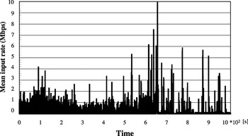
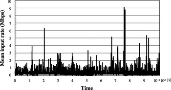
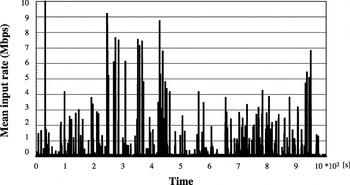
In this section, we present the tightness of Eq. (5.15) using numerical experiments we conducted by simulation. The simulation was conducted based on three sets of actual traffic data (datasets 1, 2, and 3), which were collected on a 100-Mbps Ethernet in Chiba University. Each dataset consists of the lengths and arrival times of packets that were seen on the Ethernet for 4000 s. Figures 1, 2, and 3 respectively depict sequences of simple plots of mean input rate for datasets 1, 2, and 3, where the mean input rate is defined by

Figures 1, 2, and 3 confirm that the traffic recorded in each dataset is very bursty and has a nature typical of local area network (LAN) traffic (see Leland, Taqqu, Willinger, and Wilson [5]).

Mean input rate per 100 ms: Dataset 1.

Mean input rate per 100 ms: Dataset 2.

Mean input rate per 100 ms: Dataset 3.

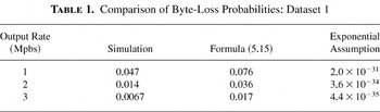
Comparison of Byte-Loss Probabilities: Dataset 1

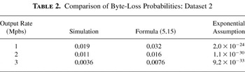
Comparison of Byte-Loss Probabilities: Dataset 2

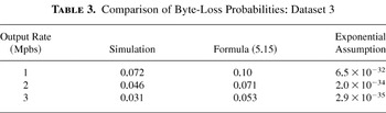
Comparison of Byte-Loss Probabilities: Dataset 3

In the simulation, we sequentially generated packets based on dataset 1, 2, or 3, and inputted them into a single-server queue that had a buffer space of 125 kbytes. Then, we counted the total size of packets that were lost by buffer overflow and obtained the byte-loss probability (BLP), which is defined by

(Note that the BLP corresponds to the work loss probability defined in Section 5.) To precisely emulate an actual packet-handling procedure, we applied the whole acceptance rule—a packet would be lost if the unoccupied buffer space was less than the size of the packet upon its arrival—to the simulation.

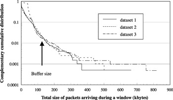
To evaluate the BLP using Eq. (5.15), dividing the time axis into fixed-length windows, we sequentially observed the total size of packets arriving at each window in the simulation. Based on the observed data, we then evaluated the right-hand side of Eq. (5.15), assuming that packets arrived in a batch at the beginning of each window. (Note that under this assumption, the nth customer of the model used in previous sections corresponds to the batch of packets arriving during the nth window. Thus, the size of work of the nth customer X_n is equal to the total size of packets arriving at the nth window, and the interarrival time between the nth and (n + 1)st customers U_n is equal to the length of the window.) Figure 4 depicts the complementary cumulative distributions of the total size of packets arriving at each window. Figure 4 reveals that all of the datasets have similar complementary cumulative distributions.

Complementary cumulative distribution of the total size of packets arriving at a window.

Tables 1, 2, and 3 respectively show BLPs obtained by simulation for different values of output rate from the queue for datasets 1, 2, and 3. Tables 1, 2, and 3 also show the bounds of BLP, which we evaluated by setting T = B/C in Eq. (5.15), where B is the buffer size and C is the output rate. For comparison, in these tables, we furthermore show the BLP evaluated under the assumption that packets arrived according to a Poisson process, the interarrival times of packets were exponentially distributed and the partial acceptance rule was applied. (We refer to this assumption as the “exponential assumption.”) Under the exponential assumption, the BLP is given by

where L is the mean size of packet and τ is the mean interarrival time of packets (see Takács [12]). Tables 1, 2, and 3 show that the exponential assumption yielded overly optimistic estimates of BLP. In contrast, Eq. (5.15) gave much better estimates of BLP with accuracy sufficient for practical use.

Remark 6.1: If we know the distribution of the interarrival time of packets and that of the size of packets, we can evaluate the bounds of BLP using Eq. (5.14), where F corresponds to the distribution of the size of packets and G corresponds to the distribution of interarrival time of packets. In general, however, such use of Eq. (5.14) does not give tight bounds of BLP. In addition, the distribution of interarrival time of packets is not easy to observe because a packet analyzer with fine-time resolution is required for observation.

7. CONCLUDING REMARK

In this article, we compared the queues whose work processes or interarrival processes are directionally convex ordered. In particular, we showed that if the work processes are directionally convex ordered, so is the amount of work lost (processed) in the systems. Similarly, we showed that if the interarrival processes are directionally convex ordered, so is the amount of work lost (processed) in the systems. Using these results, we established the formula that gives the upper bound of work-loss probability based only on the marginal distributions of work and interarrival processes.

As noted in Remark 3.2, although most of the results derived in this article seem intuitive, those do not generally hold when the whole acceptance rule is applied. However, if relevant queue management is applied, the results in Sections 3 and 4 still hold even when the whole acceptance rule is applied. Let us consider the case where the maximum size of work of a customer is finite. (For example, the maximum size of a packet is 1514 bytes in Ethernet.) In such a case, we could show that the results in Sections 3 and 4 still hold if the buffer reservation—the customer is accepted only when the unoccupied buffer is greater than the maximum size of work—is applied to the queue.

Acknowledgment

We thank Professor Tetsuya Takine for his helpful comments on this work.

References

REFERENCES

Chang, C.S., Chao, X.L., & Pinedo, M. (1991). Monotonicity results for queues with doubly stochastic Poisson arrivals: Ross's conjecture. Advances in Applied Probability 23: 210–228.Google Scholar

Chang, C.S., Chao, X.L., Pinedo, M., & Shanthikumar, J.G. (1991). Stochastic convexity for multidimensional processes and its applications. IEEE Transactions on Automatic Controls 36: 1345–1355.Google Scholar

Gani, J. & Prabu, N.U. (1957). Continuous time treatment of a storage problem. Nature 182: 39–40.Google Scholar

Gani, J. & Prabu, N.U. (1958). Remarks on the dam with Poisson type inputs. Australian Journal of Applied Science 10: 113–122.Google Scholar

Leland, W.E., Taqqu, M.S., Willinger, W., & Wilson, D.V. (1994). On the self-similar nature of Ethernet traffic. IEEE/ACM Transactions on Networking 2(1): 1–15.Google Scholar

Jean-Marie, A. & Liu, Z. (1992). Stochastic comparison for queueing models via random sums and intervals. Advances in Applied Probability 24: 960–985.Google Scholar

Meester, L.E. & Shanthikumar, J.G. (1993). Regularity of stochastic processes. Probability in the Engineering and Informational Sciences 7: 343–360.Google Scholar

Miyazawa, M. & Shanthikumar, J.G. (1991). Monotonicity of the loss probabilities of single server finite queues with respect to convex order of arrival or service processes. Probability in the Engineering and Informational Sciences 5: 43–52.Google Scholar

Shaked, M. & Shanthikumar, J.G. (1994) Stochastic orders and their applications. San Diego, CA: Academic Press.

Shanthikumar, J.G. (1994). Convexity of single stage queueing systems with bulk arrivals. Queueing Systems 16: 287–299.Google Scholar

Stoyan, D. (1983). Comparison methods for queues and other stochastic models. New York: Wiley.

Takács, L. (1974). A single-server queue with limited virtual waiting time. Journal of Applied Probability 11: 612–617.Google Scholar

Takada, H. (2001). Markov modulated fluid queues with batch fluid arrivals. Journal of Operations Research Society of Japan 44(4): 344–365.Google Scholar

Takada, H., & Miyazawa M. (2001). A Markov modulated fluid queue with batch arrivals and preemption. IEICE Technical Report IN-2001-25, pp. 9–16. Tokyo: Institute of Electronics, Information, and Communication Engineers.

Toyoizumi, H., Shanthikumar, J.G., & Wolff, R.W. (1997). Two extremal autocorrelated arrival processes. Probability in the Engineering and Informational Sciences 11: 441–450.Google Scholar