INTRODUCTION
Our research focused on the Middle and Upper Pleniglacial. The Interpleniglacial period (which corresponds to Marine Isotope Stage (MIS) 3, ca. 57–29 ka, Lisiecki and Raymo Reference Lisiecki and Raymo2005) was characterized by numerous rapid climate changes (on annual to decadal timescales), long-term (centennial to millennial) climatic oscillations and extreme environmental changes, known as Dansgaard-Oeschger (D-O) cycles as recorded in Greenland ice cores (Dansgaard et al. Reference Dansgaard, Johnsen, Clausen, Dahl-Jensen, Gundestrup, Hammer, Hvidberg, Steffensen, Sveinbjörnsdottir, Jouzel and Bond1993; Huntley et al. Reference Huntley, Alfano, Allen, Pollard, Tzedakis, de Beaulieu, Grüger and Watts2003; Wohlfarth et al. Reference Wohlfarth, Veres, Ampel, Lacourse, Blaauw, Preusser, Andrieu-Ponel, Kéravis and Lallier-Vergès2008). These cycles involved strong changes in the Northern Hemisphere air temperature, hydroclimate, and atmospheric circulation transitioning in a matter of decades (Sadatzki et al. Reference Sadatzki, Dokken, Berben, Muschitiello, Stein, Fahl, Menviel, Timmermann and Jansen2019). In turn, the interval ca. 29–14 ka BP (which corresponds to MIS 2) was characterized mainly by severe climatic conditions.
The recognition of rapid climate oscillations in the isotopic data from the cave speleothems in various worldwide locations, such as: the Villars Cave, SW France (Genty et al. Reference Genty, Blamart, Ouahdi, Gilmour, Baker, Jouzel and Van-Exter2003), the Kleegruben Cave, Austria (Spötl et al. Reference Spötl, Mangini and Richards2006; Moseley et al. Reference Moseley, Spötl, Svensson, Cheng, Brandstätter and Edwards2014), the Sofular Cave, Turkey (Fleitmann et al. Reference Fleitmann, Cheng, Badertscher, Edwards, Mudelsee, Göktürk, Fankhauser, Pickering, Raible, Matter, Kramers and Tüysüz2009), the Hulu Cave, China (Wang et al. Reference Wang, Cheng, Edwards, An, Wu, Shen and Dorale2001), the Moomi Cave, Yemen (Burns et al. Reference Burns, Fleitmann, Matter, Kramers and Al-Subbary2003) the Fort Stanton Cave, New Mexico, USA (Asmerom et al. Reference Asmerom, Polyak and Burns2010) and also cryogenic cave carbonate (CCC) data from caves located in Germany, the Czech Republic, Slovakia and Poland (Žák et al. Reference Žák, Richter, Filippi, Živor, Deininger, Mangini and Scholz2012), as well as data from locations such as La Grande Pile, France (Beaulieu and Reille Reference De and Reille1992), the Eifel, Germany (Sirocko et al. Reference Sirocko, Knapp, Dreher, Förster, Albert, Brunck, Veres, Dietrich, Zech and Hambach2016), Tenaghi Philippon, Greece (Pross et al. Reference Pross, Koutsodendris, Christanis, Fischer, Fletcher, Hardiman, Kalaitzidis, Knipping, Kotthoff, Milner, Müller, Schmiedl, Siavalas, Tzedakis and Wulf2015), and Lake Van, Turkey (Çağatay et al. Reference Çağatay, Öğretmen, Damci, Stockhecke, Sancar and Özeren2014), firmly support the hypothesis that the D-O cycles recorded in the Greenland ice cores may also be recorded in sediments in Poland territory. Such an assumption is also justified by the fact that very rapid changes in the Late Glacial/Holocene transition recorded in the Greenland ice cores were also recognized in Poland, e.g., in the sediments of Lake Gościąż (Goslar et al. Reference Goslar, Kuc, Ralska-Jasiewiczowa, Różański, Arnold, Bard, van Geel, Pazdur, Szeroczyńska, Wicik, Wiȩckowski and Walanus1993), the Koźmin Las site (Dzieduszyńska et al. Reference Dzieduszyńska, Kittel, Petera-Zganiacz, Brooks, Korzeń, Krąpiec, Pawłowski, Płaza, Płóciennik, Stachowicz-Rybka and Twardy2014) or the Żabieniec (Twardy et al. Reference Twardy, Żurek and Forysiak2010) and Trzechowskie (Słowiński et al. Reference Słowiński, Zawiska, Ott, Noryśkiewicz, Plessen, Apolinarska, Rzodkiewicz, Michczyńska, Wulf, Skubała, Kordowski, Błaszkiewicz and Brauer2017) paleolakes. Therefore, it seems that such environments could register the same cycles of warming and cooling as those recorded in ice cores for the earlier period of MIS 3–2. It should be noted that previous studies for the Subcarpathian Basins (Gębica et al. Reference Gębica, Michczyńska and Starkel2015; Starkel et al. Reference Starkel, Michczyńska and Gȩbica2017), for which we have numerous investigated sites and dates, as well as research in the Holy Cross Mountains (Ludwikowska-Kędzia Reference Ludwikowska-Kędzia2000, Reference Ludwikowska-Kędzia2018), showed that collective reconstructions (including analyses of summed probability density distributions of radiocarbon and luminescence dates) can help to identify warming-cooling periods during the Interpleniglacial.
The present research concerns selected regions of Poland to the south of the last glaciation’s maximum range (LGM). The main goals of our research were to check whether the proposed collective analysis method could be useful in verifying the number of “warming-cooling” cycles, recorded during the MIS 3–2 period in various sedimentary environments, and to compare the reconstructed oscillations to changes registered in Greenland ice cores.
RESEARCH AREA
Poland is located mainly in the Central European Lowlands, between the Carpathian and Sudeten Mountains to the south and the Baltic Sea to the north in the range of mid-latitudes between 49°00'N and 54°50'N and longitudes 14°07'E and 24°09'E. Poland lies in a temperate climate zone with transitional features—over the territory of Poland, humid air masses, coming from the Atlantic Ocean, clash with drier masses of continental origin.
During the Interpleniglacial, climatic conditions were influenced by the inflow of cold air masses. Atmospheric circulation was disturbed due to the progressive trend of the Scandinavian ice sheet to block the westerly wind pattern. Consequently, continentalism increased, accompanied by the lowering of mean temperatures of the warmest and coldest months as well as lower precipitation. Extreme cooling and dryness were associated with the MIS 2 period (Marks et al. Reference Marks, Makos, Szymanek, Woronko, Dzierżek and Majecka2019).
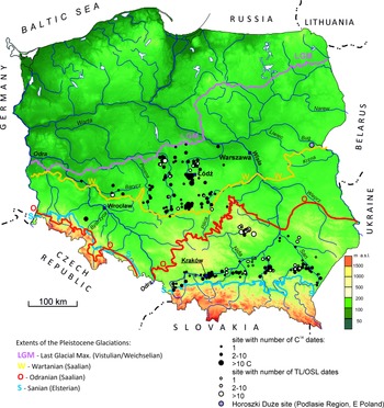
The sites selected for the analyses were located in Central and Southern Poland (Figure 1), mainly within river valleys, but also including some valley slopes and water reservoirs. These sites were beyond the reach of the LGM and were therefore more easily accessible for exploration. The choice of sedimentation environments from which the available 14C and TL/OSL dates of the sediments were compiled and analyzed was not accidental. In the selection process, we were guided by their regular functioning and the specificity of the reactions of each of them to changes in climatic conditions. Some sites and group of sites had already been analyzed by the authors: one site in the Sudeten Foreland (Krzyszkowski et al. Reference Krzyszkowski, Choma-Moryl, Kuszell, Malkiewicz and Pazdur1995, Reference Krzyszkowski, Alexandrowicz, Bluszcz, Choma-Moryl, Czeczuga, Hercman, Jędrysek, Kuszell, Nawrocki, Pazdur, Pazdur, Bluszcz, Stankowski and Starkel1999, Reference Krzyszkowski, Alexandrowicz, Bluszcz, Choma-Moryl, Goslar, Hercman, Jędrysek, Nawrocki, Pazdur and Krzyszkowski2001), numerous sites from the Subcarpathian Basins (Gębica et al. Reference Gębica, Michczyńska and Starkel2015; Starkel et al. Reference Starkel, Michczyńska and Gȩbica2017), the Holy Cross Mountains in the highlands of southern Poland (Ludwikowska-Kędzia Reference Ludwikowska-Kędzia2018), and the lowlands of central Poland (Rotnicki Reference Rotnicki1987; Krzyszkowski Reference Krzyszkowski1990, Reference Krzyszkowski1991; Kasse et al. Reference Kasse, Huijzer, Krzyszkowski, Bohncke and Coope1998; Petera Reference Petera2002; Krzyszkowski and Kuszell Reference Krzyszkowski and Kuszell2007; Wachecka-Kotkowska et al. Reference Wachecka-Kotkowska, Krzyszkowski, Klaczak and Król2014, Reference Wachecka-Kotkowska, Krzyszkowski, Malkiewicz, Mirosław-Grabowska, Niska, Krzymińska, Myśkow, Raczyk, Wieczorek, Stoiński and Rzodkiewicz2018; Dzieduszyńska Reference Dzieduszyńska2019). However, no collective analysis of this data has ever been made.
The research area with marked sites from which the analyzed dates were derived. Additionally, the location of the Horoszki Duże site was marked.

METHODS
Only one site within Poland with a probably continuous record for the analyzed time is known—Horoszki Duże (eastern Poland, Podlasie). Here, palynological studies, the analysis of macroscopic plant remains, and lithological analyses were performed and showed the presence of five interstadials between 60 and 25 thousand years ago: Oerel, Glinde, Moershooft, Hengelo, and Denekamp (Granoszewski Reference Granoszewski2003). Unfortunately, no high-resolution multi-proxy analyses were carried out—the palynological analyses were performed with low resolution (every 10 cm) and only one radiocarbon age determination was made. Other sites of terrestrial sediments from Poland formed during MIS 3–2 have even poorer data. In such a situation, we decided to perform a collective analysis of the available data from individual sites and to try to find compatible signals.
This research is a type of so-called “data mining”, analyzing 14C and luminescence dates determined in previous studies (see Supplement). Some of the dates from the Łódź region have not been published before. From the mentioned areas, we collected and verified data regarding numerous radiocarbon and luminescence dates in the range of 10–50 ka BP. Open dates (of the type “older than”) were excluded from the analyses. One site, Koźmin Las in central Poland, had many radiocarbon age estimates of wood found in the common layer. It was decided to exclude duplicate dates from this position from the analyses. Ultimately, 488 radiocarbon dates and 179 luminescence dates were selected for further analysis—see Supplement 1.
The tools used were analysis of probability density functions (PDFs) (Michczyńska et al. Reference Michczyńska, Michczyński and Pazdur2007; Gębica et al. Reference Gębica, Michczyńska and Starkel2015; Starkel et al. Reference Starkel, Michczyńska, Gębica, Wieczorek, Krzyszkowski, Michczyński, Wachecka-Kotkowska, Ludwikowska-Kędzia, Superson, Ludwikowska-Kędzia and Wiatrak2018; Dzieduszyńska Reference Dzieduszyńska2019) and also the kernel density estimation (KDE) model (Bronk Ramsey Reference Bronk Ramsey2017). PDFs and KDE models were constructed using the OxCal 4.4.4 package (Bronk Ramsey Reference Bronk Ramsey2009) employing the most recent calibration curve IntCal20 (Reimer et al. Reference Reimer, Austin, Bard, Bayliss, Blackwell, Bronk Ramsey, Butzin, Cheng, Edwards and Friedrich2020) and the corresponding commands “Sum” and “KDE model”. The constructed dates frequency distributions were then compared with the high precision δ18O Greenland ice core data (Rasmussen et al. Reference Rasmussen, Bigler, Blockley, Blunier, Buchardt, Clausen, Cvijanovic, Dahl-Jensen, Johnsen and Fischer2014). The analysis was limited to the range of the radiocarbon method, i.e., 50 cal kBP. As warm and humid conditions favored the development of vegetation cover, we expected most 14C dates to be associated with warmer (GI) periods. In turn, the GS periods, as they favored the sedimentation of mineral deposits, we expected to be visible primarily in the accumulations of luminescence dates. In addition, researchers had (usually) limited financial resources for the dating of samples, and most often (but not always) took samples for research from places where there was a change in the type of sediment. Such places were associated with changes in environmental/climate conditions on a local or global level (e.g., GI/GS boundaries). Such preferential sampling favored our analysis. It should be noted that the dates close to the boundary were usually younger or older than the border. Only thin organic inserts in mineral sediments or vice versa gave a chance to obtain an age equal to the date associated with the event studied.
RESULTS
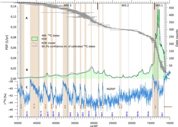
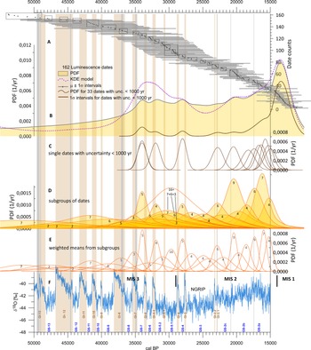
Graphical results are presented in Figure 2 for radiocarbon dates, and in Figure 3 for luminescence dates.
Analysis of 14C dates. A—each gray bar represents 68.3% confidence interval of one calibrated 14C date; B—green, filled graph—summed PDF (Bayesian approach), violet, dashed curve—KDE model (frequentist approach); C—δ18O data from Greenland ice core (Rasmussen et al. Reference Rasmussen, Bigler, Blockley, Blunier, Buchardt, Clausen, Cvijanovic, Dahl-Jensen, Johnsen and Fischer2014) with marked stadials (GS) and interstadials (GI). The boundaries of the marine isotope stages have been marked (Lisiecki and Raymo Reference Lisiecki and Raymo2005). (Please see online version for color figures.)

Analysis of luminescence dates. The timeline was narrowed to the same period as for radiocarbon dates and 17 dates from the 179 collected luminescence dates were outside of this range. A—each gray bar with a middle dot represents a 1σ interval of one luminescence date with the marked median value. B—yellow, filled graph—summed PDF (Bayesian approach), violet curve—KDE model (frequentist approach), the lowest brown curve—summed PDF for 33 dates with uncertainty < 1000 yr; C—PDFs for particular dates with uncertainty < 1000 yr; D—PDFs constructed for subgroups of luminescence dates marked by rectangles in part A; E—PDFs for weighted means from each subgroup; F—δ18O data from Greenland ice core (Rasmussen et al. Reference Rasmussen, Bigler, Blockley, Blunier, Buchardt, Clausen, Cvijanovic, Dahl-Jensen, Johnsen and Fischer2014) with marked stadials (GS) and interstadials (GI). The boundaries of the marine isotope stages have been marked (Lisiecki and Raymo Reference Lisiecki and Raymo2005). The most precise dates clearly indicate GS-7, the beginning of the GS-5.2, GS-4, changes around GI-2.2–2.1, and GS-2c/GS-2b boundary. Analysis of subgroups also shows dates that can be correlated with the GS-2b/2a boundary, GS-5.1, the end of GS-5.2 (GS-5.2/GI-5.1/GS-5.1 transition), and the beginning and the end of GS-8. GS-6 is represented by five dates but with high uncertainty, similarly GS-9 and earlier GSs. (Please see online version for color figures.)

For radiocarbon dates (Figure 2) we noted the following observations:
-
A deficit for MIS 2 dates is clearly visible in the shape of the PDF and KDE and in the position of single dates on the timeline (floating horizontal bars).
-
Almost half of all 14C dates came from GI-1–GS-1. The signal from the 15–10 cal kBP range was dominant. This range is outside the selected time interval for analysis but was included here to better illustrate the trend of the distribution of radiocarbon dates over time.
-
For ages older than 15 cal kBP, almost 10 maxima can be observed for both the PDF and KDE curves, the positions correlating well with the changes recorded in the high-precision Greenland data. This seems to indicate that the date accumulations correlate mainly with interstadial periods.
For luminescence dates (Figures 3A and B) the following observations were made:
-
A smoother curve with lower resolution compared to the 14C dates was noted, and the results of measured luminescence dates showed larger uncertainties (Figure 3A and B).
-
The largest accumulations of luminescence dates occurred for the end of MIS 3, the MIS 2 and GI-1 (Figures 3A and B).
-
The PDF distribution suggested the presence of several periods of increased accumulation of mineral deposits (one prominent and six faint peaks), while the KDE model showed five peaks in the range of 50–10 ka.
DISCUSSION
Radiocarbon Dates
The first trend, in radiocarbon dates frequency, arising from methodological considerations, was expected to be larger uncertainties and lower and smoother PDF and KDE curves with increasing ages. The results shown in Figure 2 were in line with these expectations.
The second expected trend was related to the expected frequency of dates. If there was no influence of climatic factors, we could expect that the number of dates would simply systematically decrease with increasing age as older samples were deeper in the sediments and less accessible. The results were inconsistent with such a statement, due to changes recorded in the sediments (due to changes in the sedimentation environment), additionally enhanced by preferential sampling for dating. The most interesting places for researchers were places where changes in the type of sediment were pronounced and could be selected for dating. Such preferential sampling favored the analyses performed.
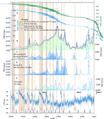
To remove the dominant influence of the large number of dates in the range of 15–11 cal kBP and better visualize the changes in the shape of the analyzed charts for 14C dates, it was best to narrow the analyzed period to 50–15 cal kBP (Figure 4).
Analysis of 14C dates. The timeline was narrowed to 15–50 cal kBP. A—upper, green floating bars: each bar represents a 68.3% confidence interval for one 14C date, lower, blue floating bars—same as above, but only for precise dates. B—green, filled graph—summed PDF (Bayesian approach), violet, dashed curve—KDE model (frequentist approach), the lowest thick, blue curve—summed PDF for precise dates; C—PDFs for dates grouping on the lower (left) boundary and during the GI periods; D—PDFs for dates grouping on the upper (right) border and during the GI periods; E—PDFs for dates during the GS periods; F—δ18O data from Greenland ice core (Rasmussen et al. Reference Rasmussen, Bigler, Blockley, Blunier, Buchardt, Clausen, Cvijanovic, Dahl-Jensen, Johnsen and Fischer2014) with marked stadials (GS) and interstadials (GI). The boundaries of the marine isotope stages have been marked (Lisiecki and Raymo Reference Lisiecki and Raymo2005). Graphs A and B show a good reflection of the following interstadials: GI-3, GI-4, GI-5.1, GI-9, GI-11 end, and the GS-2b/2a boundary. Graphs C and D indicate that each period from GI-2 to GI-12 is represented by at least a few 14C dates (above each peak, the number of dates making it up is given). Also, the GS2c/2b boundary has such a representation. Precise dates were defined as those with an uncertainty of < 1% of the age value for dates below 12 ka, 1.5% for dates ≥12 & < 13 ka, 2% for dates ≥ 13 & < 15ka, 2.5% for dates ≥15 & < 20ka, 3% for dates ≥ 20 & < 25ka 14C BP and 5% for older dates. (Please see online version for color figures.)

For the narrower period, many more details became visible. For MIS 3 we noticed six (for KDE) or nine (for PDF) well-marked peaks (Figure 4B). It was very interesting that for the younger isotopic stage, MIS 2, even the short GI-3 and GI-4 interstadials were clearly recorded by the presence of KDE and PDF maxima. The GS-2c/GS-2b and GS-2b/GS-2a boundaries were also marked with clear peaks. However, for GI-2.2 and GI-2.1, peaks before and after these interstadials could be observed.
In the collective analysis, the dates with the smallest uncertainties contributed most to the generated PDF. Therefore, Figure 4B was supplemented with a PDF curve after eliminating the dates with the highest uncertainties (the lowest curve). The shape of the PDF curve with local peaks did not change, while in Figure 4A the accumulation of dates for the GIs is more visible (lower graph). Moreover, for long GI periods, a clustering of dates at their beginning and end can be seen.
Of the 304 precise dates, 187 dates fell between 15 and 50 cal kBP. All 187 dates were assigned to subgroups based on the clusters visible in Figure 4A and Figures 4C, D, and E show the PDF distribution for these small subgroups. Figures 4C and D indicate that each period from GI-2 to GI-12 was represented by at least a few 14 C dates. The GS2c/2b and GS2b/2a boundaries also had such a representation.
Groups of dates related to stadials (Figure 4E), could also be seen, but these dates were two times less numerous. Dates within the stadials may be associated with local changes, e.g., in the fluvial environment, or with organic inserts in mineral sediments. The presence of the remains of organic matter from the GS periods was not surprising, as our research area was located in the extra-glacial zone, in places 200–250 km distant from the maximum extent of the Vistula (Weichselian) ice sheet during MIS 2 (LGM, around 24–22 cal kBP).
Luminescence Dates
The flattening of the shape of PDF and KDE curves for the luminescence dates (sediments of slope and fluvial environments), as well as the poorly readable maxima of the curves, were mainly the result of the high uncertainty values of the TL and OSL dates. However, it is noticeable in Figure 3A and B that:
-
a clear increase in the number of luminescence dates in the final phase of the MIS 3 period and the beginning of the MIS 2 period (from GS-7 to GS-4) was observed, with three peaks for the PDF curve and two for the KDE curve, covering the period of higher frequency of climate changes, i.e., alternating, short-term warm and longer cool periods,
-
an increase of both the PDF and KDE curves in the late MIS 2 period (from GI-2.2 to GI-1), with three peaks in the PDF curve and two in the KDE curve (and a very clear peak of both curves in GI-1), covering a period of long-term, stable climate conditions, i.e., the cold period (GS-2), with occasional, short-term and poorly recordable periods of changes (warming?).
In both cases, varying climatic conditions (changes in precipitation, temperature, and humidity) favored the intensive, simultaneous activation of various morphogenetic processes on the slopes (e.g., surface runoff, erosion, solifluction, active-layer detachment, high-energy overland flow, aeolian processes) and also implied changes in the dynamics of fluvial processes at the bottom of river valleys. The evidence for such changes confirms and strengthens the correctness of our results.
It is worth noting that although the differences between the GS-2 sub-events were slightly marked in the ice cores (Rasmussen et al. Reference Rasmussen, Bigler, Blockley, Blunier, Buchardt, Clausen, Cvijanovic, Dahl-Jensen, Johnsen and Fischer2014), they were clear in the reshaping of the PDF and KDE curves for luminescence dates. A slight shift of the peaks of these curves in relation to the boundaries of sub-events in GS-2 was probably related to the manner of the environments functioning on the slope/slope-valley (i.e., the record of the fluvial environment’s reaction to changes in climatic conditions may be slightly delayed in relation to the slope environment’s reaction). Both the PDF and KDE curves for the luminescence dates (based on sediments from the slope and fluvial environments), despite the large values of their uncertainties, accurately recorded the changes in the climatic conditions during the 15–50 cal kBP period.
The most reliable reconstructions require dates with low uncertainties. In the range covered by the analysis, only 33 dates had uncertainties of less than 1000 years. The analysis was supplemented with a PDF curve for the most accurate dates (the lowest curve in Figure 3B), as well as individual distributions of these dates presented in Figure 3C (20 distributions for dates with medians lower than 15 cal kBP are not included). The exact dates were in line with GS-7, GS-5.2 onset, GS-4, climate change around GI-2.2–GI-2, and the GS-2c/GS-2b boundary.
Moreover, the grouping of median distributions of single dates within individual GSs (rectangles in Figure 3A) looked intriguing. It seemed to us that due to the high uncertainties, the luminescence dates would be more dispersed. Therefore, the analysis was supplemented with PDF curves for particular subgroups of dates (see Figure 3D), as well as charts for the weighted means from particular subgroups (Figure 3E). This approach was only possible because we looked at the distribution of the luminescence dates against the background of the NGRIP curve. The dates themselves had too much uncertainty to allow for a similar definition of subgroups, but such approach showed that, starting from GS-7, each GS had related luminescence dates, and the boundaries of GS-2c/2b and GS-2b/2a were clearly marked. In the case of GS-8 and GS-5.2, the influence of preferential sampling at their beginning and end seemed to be visible.
Preferential sampling and the accumulation of dates on the boundaries of the chronozones have been observed earlier for the territory of Poland (Michczyńska et al. Reference Michczyńska, Michczyński and Pazdur2007; Michczyńska and Pazdur Reference Michczyńska and Pazdur2004). This trend was used to determine the calendar values of the chronozones boundaries for the Holocene period (Starkel et al. Reference Starkel, Michczyńska, Krąpiec, Margielewski, Nalepka and Pazdur2013).
So far, for the region of Poland, such a comprehensive analysis of the results of age determination to find a correlation with the high precision of the NGRIP curve has not been performed. However, the same type of analysis was performed earlier for the Łódź region (Dzieduszyńska Reference Dzieduszyńska2019) for Weichselian decline (18.0–11.5 cal kBP) and fluvial environment in Subcarpathian Basins (Gębica et al. Reference Gębica, Michczyńska and Starkel2015).
In the first case, the author associated the peaks of PDF curves directly with warm conditions. The current analysis prompts us to associate the accumulations of dates with transitions (e.g., glacial/interglacial or interglacial/glacial).
In the case of the analysis for the Subcarpathian Basins region (Gębica et al. Reference Gębica, Michczyńska and Starkel2015), from among several hundred available dates, only dates related to alluvial fans (42 luminescence dates and 19 14C dates) and paleomeanders abandonment events (58 14C dates) were selected for the construction of PDF curves, and the obtained results, even though presented against the NGRIP curve, were compared only with the time span of Denekamp and Hengelo interstadials.
CONCLUSIONS
-
1. The results obtained seem to show that the proposed method of a collective analysis contributes to a more complete picture of changes in the natural environment during MIS 3–2 with better resolution than before.
-
2. Collective data analysis suggests higher number of warming-cooling events than previously indicated in Poland by single records with low temporal resolution, and thus we conclude that the PDFs of radiocarbon and luminescence dates, as well as KDE models, can be useful tools.
-
3. The accumulations of radiocarbon dates correlate primarily with the interstadial periods, and the resolving power of the obtained curves is best for the youngest dates.
-
4. In the analyzed areas, the deficit of radiocarbon dates from the time corresponding to the LGM is marked. Climate and environmental changes for this period are reflected in sandy and loess (=mineral, clastic) sediments with a deficit in organics and the accumulation of luminescence dates.
-
5. The obtained results confirm the usefulness of using the collective analysis method also for luminescence dates, despite their large uncertainty range.
-
6. The juxtaposition of the absolute age of the organogenic sediments and mineral deposits allows complementary analyses, as these formations are related to rather different paleoenvironmental conditions. At times, when peat or gyttja were formed in the valleys or lakes, the accumulation of mineral deposits was suppressed and also the climate was warmer then. As opposed to these conditions, during cooler and drier times, mineral deposits (fluvial or slope) could accumulate at the expense of organic deposition.
-
7. In the case of the analyzed data from Poland, one should not expect a perfect fit of the PDF and KDE curves to the NGRIP curve image. Certain paleoenvironmental changes in Poland, due to its different geographic location, may have occurred later than they were recorded in Greenland. Unfortunately, the resolution of our analyses does not allow conclusions as to the simultaneity of changes in Poland and Greenland. Possible delays in the reaction of the environment are smaller than the resolution of our analyses. Moreover, the position of the maximum in PDF curves may also be affected by sampling for dating (before or after the change).
-
8. High precision AMS dates are very desirable in the type of analysis employed and can be helpful in finding possible instances of the leading and lagging of Polish records compared to Greenland data. For the current data, the resolution of the reconstruction is too low for this type of inference. The question is whether it will be possible at all. In this type of analysis, the shape of the calibration curve may be decisive, which, even for precise radiocarbon dates, can give wide probability distributions on the scale of calendar years.
The coincidence of maxima on the analyzed distributions for radiocarbon dates and boundaries of interstadials on the Greenland isotope curve is not yet evidence that interstadials have been identified. Further work is needed to determine whether the accumulation periods of dates are synonymous with interstadials. We intend to find palynological information and verify this for sites where it is possible. We are also going to conduct analysis for smaller regions, and for different sedimentary environments (fluvial, slope, aeolian, peatbogs and lacustrine). In the future interpretation of radiocarbon and luminescence data, it will be necessary to take into account the type of morphogeneous environment and the specificity of the record of changes with respect to climatic conditions within it.
ACKNOWLEDGMENTS
The research was supported by the SUT subsidy for the maintenance and development of research potential (14/020/BK_21/0007). Six luminescence and two radiocarbon dates from sites Swędów and Warenka were obtained in the frame of the grant UMO-2016/21/b/ST10/02451 financed by National Science Center in Poland. The authors would like to thank all reviewers for their really helpful and insightful reviews.
Supplementary material
To view supplementary material for this article, please visit https://doi.org/10.1017/RDC.2022.69.