

Introduction
A key question shared between earth systems dynamics and evolutionary biology is what drove large-scale changes in biota. Climate change, tectonics, sea-level changes, and orogeny are some environmental drivers that have been put forth as potential drivers of diversification patterns (Miller and Mao Reference Miller and Mao1995; Erwin Reference Erwin2009; Mayhew et al. Reference Mayhew, Bell, Benton and McGowan2012), but the evolution of antagonistic or symbiotic clades (Sepkoski Reference Sepkoski1996; Jablonski Reference Jablonski2008; van der Niet and Johnson Reference van der Niet and Johnson2012) and key traits (Losos Reference Losos2010) have also gained ground as important driving forces on geological timescales. However, answering questions of correlation and causality in the deep past is fraught with many different types of difficulties, including biased sampling in the fossil record, estimating relevant paleoenvironmental and biotic proxies at the appropriate scales, and erecting models appropriate to the data and the questions.
We recently suggested that higher bivalve extinction rates causally led to higher brachiopod origination rates over the Phanerozoic and that several paleoenvironmental proxies commonly invoked to be correlated with diversity had no detectable relationship to bivalve or brachiopod diversification (Liow et al. Reference Liow, Reitan and Harnik2015). We carefully dealt with the issues of biased sampling in the fossil record by simultaneously estimating sampling, extinction, and origination rates and also applied time series approaches, namely linear stochastic differential equations (SDEs), suitable for disentangling correlative versus causal relationships between time series (see “Materials and Methods”). However, one important issue remained untreated in our previous analyses. As is commonly practiced in paleontology, we examined each pair of time series in turn and evaluated the statistical support of the null, correlative, and causal relationships between them. Such pairwise (bivariate) analyses can be problematic, because the influence of other time series (in the global analysis) on the pair under consideration is ignored. In reality, a third or fourth time series, considered in an all-against-all (multivariate) analysis, could explain the apparent connection between the focal pair, if considered simultaneously. In addition, the internal mechanics of each focal pair can be better resolved by considering the influence of other time series, enabling us to detect relationships that would otherwise have been left concealed.
Here, we reanalyze four previously estimated diversification time series (Liow et al. Reference Liow, Reitan and Harnik2015), namely, brachiopod and bivalve extinction and origination rates, in multivariate analyses in order to drastically improve the credibility of our inferences. Because we found that brachiopod and bivalve sampling rates also had statistical relationships to their diversification rates (Liow et al. Reference Liow, Reitan and Harnik2015: Table S7), we also included these two time series in our new analyses. We sought to answer questions such as whether bivalve extinction rates truly drove brachiopod origination rates, or whether brachiopod origination rates were actually regulated via their own extinction rates and only apparently driven by bivalve extinctions. We infer that brachiopod and bivalve diversification rates are linked by processes likely relating to both geological and biological dynamics, operating on very different timescales; uncover a probable, yet unmeasured, driver of brachiopod extinction rates; and discuss the nature of our time series tool and the implications of our findings.
Materials and Methods
Data
We use estimates of log genus extinction, origination, and sampling rates (presented and available in Liow et al. Reference Liow, Reitan and Harnik2015) for brachiopods and bivalves over the Phanerozoic. All analyses are based on these log rates, but we refer these simply as “rates” or “time series” throughout in the interest of brevity. To briefly recapitulate, we downloaded data from the Paleobiology Database for all available data for the two clades in marine deposits, arranged the raw data such that each genus is represented by observations or nonobservations in 86 international stages, and subjected these data to capture–mark–recapture analyses. We used the Pradel seniority model (Pradel Reference Pradel1996) and simultaneously estimated extinction, origination, and sampling rates separately for brachiopods and bivalves. This approach has been previously applied to Ordovician taxa (Connolly and Miller Reference Connolly and Miller2001a,Reference Connolly and Millerb, Reference Connolly and Miller2002) and Neogene carnivorans (Liow and Finarelli Reference Liow and Finarelli2014; Finarelli and Liow Reference Finarelli and Liow2016), among other taxa, and demonstrates similarities in its estimates to more commonly used approaches (Liow and Finarelli Reference Liow and Finarelli2014) but also has differences because of the explicit modeling of sampling. Since none of the global paleoenvironmental time series available to us, namely low-latitude δ18O, δ13C, δ34S, and 87Sr/86Sr (Prokoph et al. Reference Prokoph, Shields and Veizer2008) and sea-level changes (Cardenas and Harries Reference Cardenas and Harries2010) had any detectable influence on our any of the biotic time series in pairwise comparisons (Liow et al. Reference Liow, Reitan and Harnik2015), these are not considered further here. In theory, multivariate analyses including these paleoenvironmental time series could help us detect previously undetected (weak) relationships with diversification time series. However, there is a vanishingly small chance of recovering in the multivariate analyses any paleoenvironmental-to-diversification relationships strong enough to make a difference in the detection of connections among our diversification series yet still left undetected in pairwise analyses.
Stochastic Differential Equations as a Time Series Tool for Fossil Time Series
Linear SDEs have a relatively long history in evolutionary modeling (Lande Reference Lande1976; Raup Reference Raup1977). We use linear SDEs as a time series tool here (Øksendal Reference Øksendal2010; Reitan et al. Reference Reitan, Schweder and Henderiks2012) for the following reasons. First, SDEs allow us to differentiate between correlative and causal relationships among time series, unlike regression methods (for simulations, see Liow et al. Reference Liow, Reitan and Harnik2015). Second, unlike many time series analysis tools that operate on the assumption that temporal measurements are regularly spaced, SDEs can handle those that are irregularly spaced, as is typical for fossil time series such as those we used here. As such, two time series that are suspected to be related do not need to be measured at the same time points for analyses relating them to be carried out, as long as there is some temporal overlap. Third, linear SDEs are amenable to an algorithm called Kalman filtering (Särkkä et al. Reference Särkkä, Vehtari and Lampinen2004) that can incorporate crucial information on uncertainties, regardless of whether uncertainty estimates are empirically estimated or not. In our case, we do have these uncertainty estimates available. Fourth, SDEs also allow us to model hidden or latent time series that we cannot or have not measured (“Exploring Hidden Time Series Using SDEs”).
Linear SDEs are considerably less familiar to paleobiologists than are approaches such as the Pradel model for simultaneously estimating diversification and sampling rates, hence we describe them in some detail here. The simplest, single-layered linear SDE is an Ornstein-Uhlenbeck (OU) process (Lande Reference Lande1976), which describes a mean-reverting process that reduces to a Wiener process (Brownian motion [BM]) if the deterministic part of the process is zero:
 $$dX\left( t \right)\,{\equals}\,{\minus}\alpha \left( {X\left( t \right){\minus}\mu } \right)dt{\plus}\sigma dB_{t} $$
In this SDE form of the OU process, μ is the expected value of the process, α is the mean-reverting parameter that determines the autocorrelation function, ρ(t)=cor(X(0),X(t))=e
–αt
, and α together with σ determines the stationary standard deviation
 $${{sd\left( {X\left( t \right)} \right)\,{\equals}\,\sigma } \mathord{\left/ {\vphantom {{sd\left( {X\left( t \right)} \right)\,{\equals}\,\sigma } {\sqrt {2\alpha } }}} \right. \kern-\nulldelimiterspace} {\sqrt {2\alpha } }}$$
. Equation 1 has a deterministic part, −α(X(t)−μ)dt, that describes a movement back to the expected value μ with a speed proportional to α and the current distance between process and μ. The stochastic part, σdB
t
, describes the random deviations from one instant to the next. We can reparametrize α using half-life, t
1/2=log(2)/α, that is the time needed for the deviation of the process X from the expectation μ to drop to half its previous value. Similarly, the stationary standard deviation of the process,
 $s\,{\equals}\,\sigma \sqrt {{{t_{{1\,/\,2}} } \mathord{\left/ {\vphantom {{t_{{1\,/\,2}} } {2{\rm log}\left( 2 \right)}}} \right. \kern-\nulldelimiterspace} {2{\rm log}\left( 2 \right)}}} $
, is easier to interpret than σ. The OU process has also been used quite extensively to model stasis and deviations thereof in phenotypic evolution (e.g., Hunt Reference Hunt2007).
When a given time series is subject to a linear SDE analysis, in isolation, we can extract characteristics of its behavior, including the half-life of the process, the expected value of the process, and its stationary standard variation (see paragraph above).
Modeling Links between Time Series with Linear SDEs and the Meaning of Causality in This Context
Two linear SDEs can be connected by making the stochastic part for each process correlated
 $$\hskip-5.3pc dX\left( t \right)\,{\equals}\,{\minus}\alpha _{x} \left( {X\left( t \right){\minus}\mu _{x} } \right)dt{\plus}\sigma _{x} dB_{t}^{{\left( x \right)}} $$
 $$\eqalignno{ dY\left( t \right)\,{\equals}\,&{\minus}\alpha _{y} \big( {Y\left( t \right){\minus}\mu _{y} } \big)dt{\plus}\sigma _{y} \left( {1{\minus}\rho ^{2} } \right)^{{0.5}} dB_{t}^{{\left( y \right)}} \cr&{\plus}\rho \sigma _{y} dB_{t}^{{\left( x \right)}} $$
where ρ describes the strength of the correlation between X and Y, where X may represent paleoclimate and Y may represent net diversification rates of a given clade. One can think of dX(t) as “change in X over time dt,” although the mathematical interpretation is a bit more involved.
X and Y can also be described as having a causal link from one process to the other:
 $$dX\left( t \right)\,{\equals}\,{\minus}\alpha _{x} \big( {X\big( t \big){\minus}\mu _{x} {\minus}\beta \big( {Y\big( t \big){\minus}\mu _{y} } \big)} \big)dt{\plus}\sigma _{x} dB_{t}^{{\left( x \right)}} $$
 $$\hskip-5pc dY\left( t \right)\,{\equals}\,{\minus}\alpha _{y} \big( {Y\left( t \right){\minus}\mu _{y} } \big)dt{\plus}\sigma _{y} dB_{t}^{{\left( y \right)}} $$
In this case, process X(t) is not pulled toward the expected value μ x but toward values that depend on the current state of Y(t), namely μ x −β(Y(t)−μ y). Since it takes t 1/2,x =log(2)/α x for X(t) to be pulled halfway toward this new attractor, and Y(t) has, in the meanwhile, changed, X(t) is expected to lag behind Y(t). This describes a Granger causal link (Granger Reference Granger1969; Schweder Reference Schweder1970) from Y(t) to X(t), where β describes the strength of this relationship. Where a Granger causal link is demonstrated, it means that the driver contains information to probabilistically “predict” what happens to the “driven time series” later. However, note that because we can never take into account all other relevant factors that have influenced the “driven time series,” we cannot confirm that the driver truly directly (i.e., proximately) caused the driven time series. We will instead term a link “direct” if there is no detectable measured or unmeasured process in between the driver and the driven series. We are also unable to infer probable mechanisms based only on SDEs. Speculations on mechanisms, however, can be based on links and parameters inferred by SDEs. What true causality is and whether we can ever truly infer true causal links are the subjects of huge statistical and philosophical literatures that are beyond the scope our discussion (Eichler Reference Eichler2013). However, for the rest of our paper, we simply use the term “causality” to mean Granger causality and the term “driver” as implied by modeling Granger causality using linear SDEs as a tool.
By explicitly modeling one time series as a driver of a second time series, we can further estimate characteristics of these time series given the model, and we can compare such a model with others (e.g., null model of no relationship, correlative model, causal model where Y drove X or vice versa) using information criteria (such as Akaike information criterion) or Bayesian model probability, calculated using Bayesian model likelihood (BML, also known as prior predictive likelihood).
Exploring Hidden Time Series Using SDEs
It is possible to detect the effect of a causal driver of a time series, even when that causal driver is not measured, that is, it is “hidden” in the time series. A hidden time series is part of a multilayered structure of cause and effect and can be either a direct or a distal cause of the time series in question (Reitan et al. Reference Reitan, Schweder and Henderiks2012), depending on where in the chain of causality it is found. The corresponding SDEs therefore will be encapsulated in casual layers. Expanding on equation 1, where X was described as an OU process, we can replace μ by a time-varying term X 2 , such that it becomes OU-like (eq. 6), and X 2 itself is controlled by X 3 (described in eq. 8). We therefore rename X as X 1 for clarity. X 2 and X 3 do not have to be measured or observable. We illustrate X 1 and X 2 as OU-like processes and X 3 as an OU process here, but these can also take other forms, such as an OU process with a linear time trend or a BM process. Note, however, that a BM process cannot be driven by another underlying process, although it can drive processes “above” it.
 $$dX_{1} \left( t \right)\,{\equals}\,{\minus}\alpha _{1} \left( {X_{1} \left( t \right){\minus}X_{2} \left( t \right)} \right)dt{\plus}\sigma _{1} dB_{t}^{{\left( 1 \right)}} $$
 $$dX_{2} \left( t \right)\,{\equals}\,{\minus}\alpha _{2} \left( {X_{2} \left( t \right){\minus}X_{3} \left( t \right)} \right)dt{\plus}\sigma _{2} dB_{t}^{{\left( 2 \right)}} $$
 $$dX_{3} \left( t \right)\,{\equals}\,{\minus}\alpha _{3} \left( {X_{3} \left( t \right){\minus}\mu } \right)dt{\plus}\sigma _{3} dB_{t}^{{\left( 3 \right)}} $$
It is not possible to simultaneously identify the connection strength and the variance of the underlying hidden process. Similarly, one cannot assign separate expected values to each process in a line of hidden layers. We set the expected value of the bottom layer (which will then transfer to all the layers above) and the connection strengths to one (β=1, hence it does not appear in eq. 7 or eq. 6), so as to remove this identifiability issue. This means that for a hidden layer, the real process described by the (inferred) hidden layer can be any linear transformation of the inferred process.
More such hidden layers can be modeled, but we stopped at two hidden layers in our application here. For more details, see Reitan et al. (Reference Reitan, Schweder and Henderiks2012).
Why Multivariate Analyses Are Needed
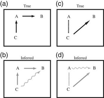
Imagine a simple pairwise analysis using linear SDE in which we have three time series of interest that we hypothesize may have relationships to one another. We may find a spurious direct causal relationship between time series C and B where there is none (or more correctly, where the causal relationship is only distal), simply because C directly drives A, which in turn directly drives B (Fig. 1a,b). In other words, the relationship between A and C and the relationship between A and B completely explain the system, and we erroneously added another direct relationship using a simple pairwise analysis. Continuing with a slightly more complicated example with three time series, assume that in reality C directly drives B but has common stochasticity with A (i.e., a correlative connection). A pairwise analysis of A and B can then easily result in the erroneous conclusion that A directly drives B, since A will look similar to the real driver of B (Fig. 1d). Note that although we illustrated why multivariate analyses are needed to avoid inferring spurious relationships (Eichler Reference Eichler2013) using SDEs, this is true even for other types of analyses, including the commonly used linear regression and other statistical approaches that probe interactions among time series.
Two examples of single-layer causal analysis with three time series. a, Illustration of the first example, in which time series A is causally driven by C but drives B (solid black lines indicate true underlying processes). b, Pairwise inference on the system illustrated in part a is correct (now colored gray because these are inferences), but additionally, C could be inferred as driving B (gray squiggle indicates spurious inference). This is because changes in C drive changes in A, which in turn drive changes in B, although there is no direct relationship between C and B as inferred. c, Illustration of the second example, in which time series C is correlated with A (dashes) but drives B (solid arrow from C to B). d, Inference from pairwise analyses in the system illustrated in part c, in which the correct correlative relationship was found between A and C but a spurious causal connection was found between A and B. This is because C and A have the same dynamics, and we are falsely led into thinking A also drove B, when only C drove B. In both examples, we assume that there are enough data to recover the true relationships if the appropriate multivariate approaches are used.

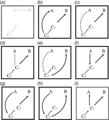
The situation gets more complex when hidden time series (see previous section) are involved. As an illustration, imagine that A is found, spuriously, to have causally driven B in a pairwise analysis as before (Fig. 2a). This time, another time series in the system has one measured layer (C1) and one hidden layer (C2). There are seven true scenarios that involve the layered series in C that can mislead us into thinking A drove B (Fig. 2b–h) if we performed only pairwise analyses, given that A and B react equally fast (measured in terms of their half-lives). More scenarios are possible if B reacts more slowly than A, as illustrated in Figure 2i.
Multilayer causal analysis with three time series. a, Illustration of the inference from a pairwise analysis in a system with three time series, in which A is falsely inferred to be driving B. For simplicity, we do not illustrate the multiple possibilities of the connections between the multilayer C process and the A and B processes in part a. b–h, The seven alternative underlying scenarios that could have led to the inference in part a, given that a pairwise analysis was performed and that A and B have comparable reaction times. Even more cases could be considered if A reacts faster than B (t 1/2,B >t 1/2, A ), such as is seen in part i. Lines as defined in Fig. 1.

In addition, the parameter values and even the structure of the time series (see “Model Selection: Workflow and Search Algorithm”) might be unstable for a given time series in pairwise analyses, if extra variation that can be explained by a third time series is not accounted for. In addition, a more consistent understanding of individual processes can be achieved by doing multivariate comparisons. For instance, if a process A drives B, but C is unconnected to either of them, a pairwise analysis of A and B will reveal that the variation of A explains some of the variation and autocorrelation of B, while a pairwise analysis of B and C will miss this element. As a result, the parameter estimates of B could be highly inconsistent from one pairwise analysis to the next.
While we cannot increase the number of time series in a given analysis infinitely due to computational time considerations, careful planning of the search through the space of plausible models is required to converge on robust results.
In summary, by going beyond pairwise analyses, we can avoid false connections, detect connections that we cannot infer in pairwise analyses, and attain a more consistent picture of the nature of each process.
Interpretation of Parameter Estimates and Link Relationships
A causal connection from Y(t) to X(t) is modeled as shown in equations 4 and 5 (Reitan et. al Reference Reitan, Schweder and Henderiks2012). However, in the case in which X(t) responds to Y(t) very rapidly (i.e., X(t) has a half-life much shorter than the smallest time resolution of the data), another interpretation is plausible but not distinguishable from causality: X(t) can be said to be the sum of Y(t) and noise (and/or other descriptors of X(t), including fast-moving autoregressive processes). In other words, X and Y are common (or shared) processes, where X is noisy while Y is noiseless. Hence, when interpreting our results, it is crucial to examine both the nature of connections and the estimated parameters.
Model Selection: Workflow and Search Algorithm
When inferring correlative connections and causality from time series, one needs to search through multiple models characterized by different connection types. Statistical model searches based on Bayesian model probability (as used here) or information criteria means searching for the most parsimonious explanation for the data. Thus, even if a model search suggests A as a direct driver of B, it could be that A drives an unknown process that drives B or that A is tightly linked to an unknown process that is a direct driver of B. Such models are, however, within the framework described, so when a more parsimonious model is chosen, it means the simpler explanation has support and there should be special reasons for contemplating more complicated explanations.
It is not feasible to explore all possible multivariate models when many time series are involved, as the number of possible combinations of layers and connection models becomes prohibitive. Thus, a stand-alone analysis of each time series was performed to determine the initial structure of each series, that is, the number of hidden layers, the stochasticity of each layer, and the nature of the lowest layer (Wiener process, OU, or linear trend plus OU). However, to allow each process to receive as well as send out causal signals, we changed the nature of the lowest layer to OU if the stand-alone analysis assigned a Wiener process to it. As the Wiener process is a subset of the OU process, and we cannot be certain that the pull parameter, α, is exactly zero, it is highly unlikely that using an OU process instead of a Wiener process has substantial consequences for the modeling of the process. However, this (substituting a Wiener process with an OU one) has the advantage of ensuring we do not miss models that are plausible in cases where α is very small but not exactly zero.
The starting point of an enhanced stepwise analysis consists of the structure of each time series (i.e., number of layers and if those are OU or other processes) from the stand-alone analyses, where none of the time series are connected. From this starting point, connections can be added, changed, or removed and the structure of each time series can be changed. For each iteration, the model with the highest BML is chosen as the input model for the next iteration. Additional connections are only accepted when the Bayes factor for an extra connection versus the input model is larger than one:
 $\hskip-9pt\eqalignno{ B_{{{\rm new}\;{\rm connection}\;{\rm vs}{\rm .}\;{\rm input}\;{\rm model}}} &\,\,{\equals}\,\,{{\mathop{\sum}\limits_{m\,{\equals}\,1}^M {P\left( m \right)P\left( {D\left| m \right.} \right)} } \over {P\left( {input} \right)P\left( {D\left| {input} \right.} \right)}}\cr&\,{\equals}\,\mathop{\sum}\limits_{m\,{\equals}\,1}^M {{{BML_{m} } \over {M^{\asterisk}BML_{0} }}}, $
where m∈{1,…,M} is the set of additional connection models. The Bayesian model likelihoods are defined as BML
m
≡P(D|m), BML
0≡P(D|input), and the prior model probabilities are set to
 $P\left( {input} \right)\,{\equals}\,{\raise0.7ex\hbox{$1$} \!\mathord{\left/ {\vphantom {1 2}}\right.\kern-\nulldelimiterspace}\!\lower0.7ex\hbox{$2$}}$
and
 $P\left( m \right)\,{\equals}\,{\raise0.7ex\hbox{$1$} \!\mathord{\left/ {\vphantom {1 {2M}}}\right.\kern-\nulldelimiterspace}\!\lower0.7ex\hbox{${2M}$}}$
(or proportional to this), so that the input model has the same prior probability as the combined set of new connection models. If there is insufficient evidence for a new connection but a change in connection nature or structure yields a higher BML than the input model, then that change will be accepted and will thus be the input model for the next iteration. If there is insufficient evidence for a new connection and no connection or structural change yield a higher BML, then the iterations stop.
To avoid misidentifying connections and to improve parameter estimates as explained earlier, we subject brachiopod and bivalve origination, extinction, and sampling rates to a multivariate linear SDE analysis in which connections among all six time series and their hidden layers were considered simultaneously. We had previously performed stand-alone analyses of each of these time series and used BML as our model-selection criterion so as to have a sketch of the rough structure of each process (Liow et al. Reference Liow, Reitan and Harnik2015).
As is clear from the number of possibilities from even a simple example with only three time series in which only one has two hidden layers (Fig. 2, a nonexhaustive illustration), the search space for models in our empirical system is very large, hence an effective search algorithm has to be designed. Hence, we devised an enhanced stepwise search algorithm. Our null hypothesis consists of the best structures from the stand-alone analyses for each time series and with no connections between any of the time series. In each of the iterations that follow, we examine a set of models and choose the model with highest BML. In doing so, new parameter values for structures of each process will also be estimated. The first step examines all models with only one connection. The second step examines models with a single connection added to the best model from the first step. The third and all subsequent steps examine models with one connection in addition to the connections in the previous step. In addition, from the third step onward, we examine models in which we changed the structure of one of the time series (e.g., single-layer OU to two hidden layers) and models in which we replaced one of the existing connection types (e.g., correlative) with another (to causal from Y to X or causal from X to Y). This additional move allows us to find models that we might otherwise miss in a simple stepwise approach and also saves time relative to a total brute-force approach. Using the described algorithm, we examined hundreds of different models that can be constructed based on six potentially interconnected time series, including models that consisted of feedback loops, which did not get selected by BML and are hence not presented. Each of these is run 10 times to ensure the stability of results. The code for linear SDE analyses is written in C++, while the code for running these analyses is written in Perl (Reitan Reference Reitan2016).
Results
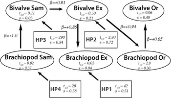
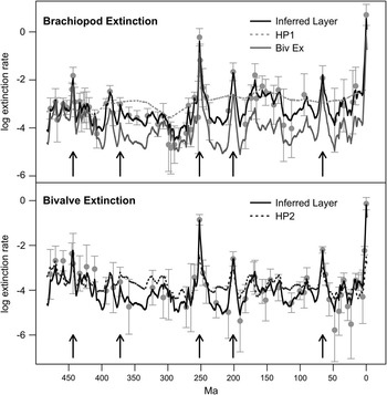
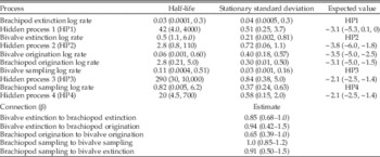
The best multivariate hidden-layer model, in which we allowed each time series to be described by at most two underlying hidden time series and in which multiple connections were examined simultaneously, confirms that high bivalve extinction drove brachiopod origination rates (Fig. 3) (Liow et al. Reference Liow, Reitan and Harnik2015). We can make this interpretation, because the half-life of brachiopod origination rate is on the order of the resolution of the data from which these rates are estimated (see “Interpretation of Parameter Estimates and Link Relationships”). The strength of this causative link (β=0.94; Fig. 3, Table 1) is similar to the one we previously estimated in a pairwise model (β=1.0 in Liow et al. Reference Liow, Reitan and Harnik2015). Two uncertain relationships that were present previously (see Liow et al. Reference Liow, Reitan and Harnik2015) vanished: namely the positive link (correlative or causal, differing between hidden and single-layer models) between brachiopod extinction and origination rates and the positive link between bivalve extinction and bivalve origination rates (Fig. 3). These previous pairwise connections are now explained by indirect connections. Bivalve and brachiopod extinction rates are linked, but whereas they were simply positively correlated in single-layer pairwise analyses (Liow et al. Reference Liow, Reitan and Harnik2015), hidden-layer analyses revealed complexity. While bivalve extinction could have driven brachiopod extinction (Fig. 3), this relationship is uncertain, because the half-life of the latter is much smaller than the resolution of the data (6.5 Myr; see Liow et al. Reference Liow, Reitan and Harnik2015). A plausible interpretation is that brachiopod extinction rates have the same dynamics as bivalve extinction rates in addition to being characterized by a slower-acting process (Fig. 3, HP1) that adds variation to bivalve extinction rates. This hidden layer (Fig. 3, HP1) is smooth and slow, with a half-life of 42 Myr (Table 1) with a clear decline during the Carboniferous that rises again after the Carboniferous/Permian boundary (Fig. 4). We also show a plot for inferred bivalve extinction rates together with its hidden process (Fig. 5, HP2): notice the similarity of inferred bivalve and brachiopod extinction rates. We infer that brachiopod originations drove bivalve originations (Fig. 3), but just as in the case of extinctions, the half-life of bivalve originations (0.06 Myr) is smaller than the resolution of our data, and hence, it is probable that bivalve originations simply mirror brachiopod originations, topped with extra statistical noise. We do not figure the origination rates, since they were already figured in Liow et al. (Reference Liow, Reitan and Harnik2015) and because they do not have hidden processes, unlike the extinction rates.
This figure shows the best multivariate model and its parameter estimates from this study. Arrows originate from drivers and end at the affected time series. Hidden processes (HP) are reported in boxes, while measured processes (Sam, sampling; Ex, extinction; Or, origination) and their inferred parameters are in ovals. All parameters are as described in “Materials and Methods.” Credibility bands are presented in Table 1.

The dynamics of the inferred processes for log brachiopod and bivalve extinction rates across the Phanerozoic are plotted. Gray dots and lines are extinction-rate estimates and their 95% confidence intervals from Liow et al. (Reference Liow, Reitan and Harnik2015) (those with SE>0.8 are not plotted). Inferred layer refers to the dynamics of extinction (black line) while hidden processes (HP1 and HP2) are the second layers (gray dotted lines). Note that the dynamics of bivalve extinction rates (Biv Ext, gray solid line in first panel and black line in second) also contribute to brachiopod rates. The estimates for bivalve extinction rates are in addition affected by bivalve sampling rates (not shown here but shown in Fig. 5). The hidden process is only known up to a linear transformation, because of issues of identifiability, which in practice means that the real process, reflected by the inferred process, can be any linear transformation of the latter. Vertical arrows indicate the temporal positions of the “big five” mass extinctions.

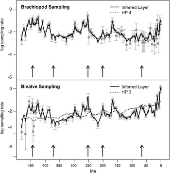
The dynamics of the inferred processes for log brachiopod and bivalve sampling rates across the Phanerozoic are plotted. Gray dots and lines are sampling-rate estimates and their 95% confidence intervals from Liow et al. (Reference Liow, Reitan and Harnik2015) (those with SE>0.8 are not plotted). Inferred layer 1 refers to the inferred dynamics of sampling (black line), while the hidden processes (HP3 and HP4, dotted lines) are the hidden layer under that. Vertical arrows indicate the temporal positions of the “big five” mass extinctions.

Estimates for best all-against-all multivariate model. In the process part of the table, half-lives (t 1/2) are in Myr, expected values and stationary standard deviations (s) have the same units as the processes themselves, and values in parentheses are 95% credibility bands. β is unitless. In the connections part of the table, β=0.94 means that if bivalve extinction-rate changes by 1 unit on a log scale, then brachiopod origination rate gradually changes by 0.94 units (also on the log scale).

While modern-day sampling cannot influence past extinction rates, sampling rate as estimated in this study is a complex proxy including true population densities, species geographic distributions, preservation processes, and geological processes in addition to modern-day sampling (see Liow et al. Reference Liow, Reitan and Harnik2015). For instance, higher true occupancy can lead to higher sampling rates (Liow Reference Liow2013), and higher occupancy can in turn confer greater resistance to local extinction or cause location extinction of competitors. Hence, it is plausible that one or more processes encompassed by the estimated bivalve sampling rate process have driven bivalve extinction rates. However the half-life of bivalve extinction is low relative to the resolution of the data used to infer these rates (Table 1, Fig. 3), so we must be open to the interpretation that bivalve sampling rates contribute noise to bivalve extinction rates and that this noise is purely inference related. Both bivalve and brachiopod sampling rates have their own hidden processes but are otherwise similar to each other (Fig. 5).
Discussion
A key goal in quantitative paleontology is to understand what drove large-scale changes in Earth’s history. Causal inferences in historical and natural sciences where controlled experiments are not possible, such as in paleontology, are challenging but have seen several recent developments. Information transfer or IT (Hlaváčková-Schindler et al. Reference Hlaváčková-Schindler, Paluš, Vejmelka and Bhattacharya2007; Hannisdal Reference Hannisdal2011), convergent cross-mapping or CCM (Sugihara et al. Reference Sugihara, May, Ye, Hsieh, Deyle, Fogarty and Munch2012; Ye et al. Reference Ye, Deyle, Gilarranz and Sugihara2015), and linear SDEs (Reitan et al. Reference Reitan, Schweder and Henderiks2012; Liow et al. Reference Liow, Reitan and Harnik2015), each with their own assumptions and caveats, are some approaches recently applied in geology and biology to differentiate correlations and causations. Here, we have chosen to parameterize our time series as a series of hidden layers where necessary, using linear SDEs. Our parametric approach revealed the nature of bivalve and brachiopod extinction rates, which drove brachiopod origination and, indirectly, bivalve origination. Such an inference would not have been possible with the nonparametric approaches of CCM and IT.
By applying multivariate modeling of a system of linear SDEs, we have simplified and clarified the processes that seem to have controlled brachiopod and bivalve diversification rates across the Phanerozoic. The extinction of bivalves freed up ecospace for brachiopods, and the origination of brachiopods in turn may have created more new ecospace for bivalves (but see below). The bivalve origination rate has a short half-life of 0.06 Myr (95% credibility interval: 1 Kyr–0.6 Myr), while the brachiopod origination rate has a half-life one order of magnitude longer at 2.8 Myr (95% credibility interval: 2.1–5.0 Myr; Table 1). Although brachiopod origination rates are inferred as driving bivalve origination rates (Fig. 3, Table 1), we interpret this as brachiopod and bivalve origination rates being very similar, with bivalve origination having a “noise” component that may be fast-acting processes, as is likely the case for the inferred relationship between bivalve and brachiopod extinction. The best model in the full model has single-layered origination processes, suggesting that originations are simply characteristics of the clades. Extinctions on the other hand may be “externally controlled,” although it is unknown what represents a control at this scale (Figs. 4, 5). Brachiopod extinction dynamics are essentially identical to bivalve extinction dynamics but are also affected by an extra process that is less temporally volatile (HP1). While we do not yet know what this process represents, it is possible to infer its dynamics (Fig. 4), which gives us clues to its possible identity. In fact, any time series that is a linear transformation of this hidden process is just as likely a candidate, including those with negative scaling, because of the previously mentioned issue of identifiability. Both bivalve and brachiopod sampling rates are driven by slower-acting underlying processes, and sampling processes in turn affect extinction processes directly or indirectly.
Sampling-rate inference is unavoidable for diversification rate inference using data from the fossil record. Sampling rates used in this study are estimated jointly with diversification rates using the same data, so this nonindependence does mean that it is inevitable that links will be found between inferred sampling rates and inferred diversification rates. This could be the whole explanation for the causal connection from bivalve sampling rates to bivalve extinction rates. However, we also note here, as we previously did (Liow et al. Reference Liow, Reitan and Harnik2015), that the sampling time series represent complex processes, including abundance, geographical spread, and preservation potentials of the living organisms as well as geological processes and present-day research efforts. Thus, whether causal or correlative, links between sampling and diversification rates as estimated here are not as unintuitive as at first glance. Using the given data and analyses, we cannot distinguish among the mechanisms of the links between sampling rates and diversification rates. For instance, bivalve extinction is a hidden layer (HP2) plus 0.91 times the bivalve sampling rate (Fig. 4). This hidden layer would then represent an extinction process not already captured by sampling rates (including temporal changes in abundance and geographical distributions). To increase our understanding of what controls extinction rates, we need to dissect complex processes that affect sampling, including geological processes, changing ecological abundance, and human effort.
In this study, we examined hundreds of different models using the six potentially interconnected time series of bivalve and brachiopod diversification and sampling. The search space for models increases more than exponentially as the number of plausibly interconnected time series linearly increases in a given system, increasing the chance of not converging on a model close to the truth. There is no easy solution to this, and we emphasize that the decision to include or exclude time series must depend on a good understanding of the system in question. We also add the caveat that our linear approach does not capture relationships among nonlinear time series, unless the nonlinearity can be removed by transformations. This problem can be alleviated using nonparametric approaches such as IT and CCM (Hannisdal Reference Hannisdal2011; Sugihara et al. Reference Sugihara, May, Ye, Hsieh, Deyle, Fogarty and Munch2012), although, as already mentioned, these approaches do not allow us to estimate parameters from the models.
These new multivariate analyses give us extra confidence that bivalves did suppress the diversification of brachiopods on geological timescales, although the underlying biological mechanisms are still elusive, as they must be unveiled using a combination of ecologically and evolutionary relevant models and empirical data.
Acknowledgments
We thank Thomas F. Hansen (University of Oslo) for spurring us to go beyond pairwise analyses and Peter J. Wagner (University of Nebraska–Lincoln) and Michael Foote (University of Chicago) for constructive reviews of this work. This research is funded by Norwegian Research Council grant 235073/F20 LINK to L.H.L. This is Paleobiology Database Publication #279.