Travel, stump speeches, and pressing-the-flesh make up a large part of any electoral campaign. Historically, we know about Abraham Lincoln and Stephen Douglas's travels throughout Illinois to debate the issues as they campaigned for Senate. More personally, the grandmother of one of the authors met a candidate in a supermarket as he campaigned in his first race for Congress. For the next 20 years, she referred to him as “that nice young man” whenever she heard his name.
To gain that level of recognition and support, presidential campaigns similarly emphasize campaign appearances. Candidates start their travels long before presidential primaries, and as the election nears, they spend more and more time on the road, visiting states where only a small push is needed to make a difference and not stopping until the election polls close. Gone are the days when the presidential candidate sipped cider on his porch and stayed out of the campaign. Instead, we now see sets of peripatetic individuals whose travel time is carefully managed and planned.
Obviously, candidates feel that their appearances are important, as they make hundreds of appearances before Election Day. But are they right? Well over 100 million people cast ballots in a presidential election. Only the tiniest fraction of this group sees either of the candidates. How effective is this type of presidential campaign activity? This question is relevant to the least, as well as the most, populous battleground states. In the 2004 election, for example, how many of New Hampshire's 675,314 voters met either candidate? As for our author's grandmother, although she developed a strong positive opinion of the candidate she met, she never voted for him, which highlights the importance of our question about the value of appearances.
We are left with a paradox. Candidates invest too much time and too many resources for us to simply conclude that campaign appearances have little or no impact on election outcomes. On the other hand, given the relatively limited numbers of people seen by a candidate, campaign appearances cannot matter very much. We investigated this apparent conundrum by gathering data on candidate appearances in battleground and non-battleground states and evaluating how these appearances influence the opinions of voters, as measured by changes in state tracking polls.
What we found is that campaign appearances can potentially have an impact on voter support, but this impact depends on both the candidate and where he or she is campaigning. Although the impact of a visit may be small, the combined impact of several appearances in a trip may be large enough to swing closely contested states toward one candidate. In our study, we also found that the impact of the vice-presidential candidate can be larger than the impact of the presidential candidate. This suggests that the choice of a vice-president is important, not necessarily because of the traditional reasons of balancing out a ticket or winning a swing state, but because of the campaigning ability of the vice-president.
THE IMPACT OF CAMPAIGNS AND CAMPAIGN APPEARANCES
Candidates and their staff invest much energy in designing campaigns, and they take particular care in planning a candidate's visits. During Jimmy Carter's first presidential campaign, for example, advisor Hamilton Jordan devised a formula to determine the best use of Carter's visits. The impacts of full-day visits to a state by the presidential candidate, the running mate, the candidates' wives, and the candidates' children were each given a different weight. Appearances were then allocated, and Jordan could track their potential impact by this point system (Witcover Reference Witcover1977, 518–20). President George W. Bush's aide and strategist Karl Rove similarly believed in the importance of campaign appearances. He described Democratic candidate Al Gore's trip down the Mississippi River as the best tactical move that the campaign made, because it generated “glowing news coverage” (Institute of Politics at Harvard University 2002). King and Morehouse sum up the view of political actors in stating that “they simply ‘know’ that candidate visits to targeted areas have a positive effect on voters” (Reference King and Morehouse2004, 4).
Unlike political actors, political scientists have been more skeptical about the importance of either campaigns or candidate appearances. For years, the dominant school of thought claimed that campaigns had a “minimal effect” on elections (see, e.g., Campbell et al. Reference Campbell, Converse, Miller and Stokes1960). While acknowledging the possibility of impact (see, e.g., Berelson, Lazarsfeld, and McPhee Reference Berelson, Lazarsfeld and McPhee1954), political scientists have traditionally believed that elections primarily activate predispositions, and their research has emphasized factors such as party affiliation, group membership, and media exposure.Footnote 1 Later, scholars shifted their focus to forecasting elections using models incorporating economic variables, presidential approval, and voting history (e.g., Tufte Reference Tufte1978; Rosenstone Reference Rosenstone1983; Lewis-Beck and Rice Reference Lewis-Beck and Rice1992).
More recent work has reexamined the “minimal effects” model and again found that campaigns serve primarily to activate preexisting dispositions, but may also create some small changes at the margin. Markus (Reference Markus1988), for example, suggests that campaigns could possibly influence 3% of the vote not accounted for by predispositions. Similarly, Finkel concludes that the “potential exists” for campaigns to change elections, and that they “could certainly swing the overall outcome of the contest” (Reference Finkel1993, 19). Other studies reach similar conclusions, but also find that campaigns have done little to change outcomes (Bartels Reference Bartels1993; Gelman and King Reference Gelman and King1993).
The minimal effects model has its critics. Holbrook challenges this approach (Reference Holbrook1994, Reference Holbrook1996) and suggests that economic conditions and presidential approval determine an equilibrium level of support, but this support fluctuates around the equilibrium “in response to campaign events,” with conventions being particularly important (Reference Holbrook and Craig2006, 5).
Of all the events that compose a campaign, however, campaign appearances are arguably the most visible and physically demanding event for a candidate. Yet, until recently, less attention has been focused on candidate campaign visits (Shaw Reference Shaw2006, 40). Using surveys from the 2000 election, Johnston, Hagen, and Jamieson (Reference Johnston, Hagen and Jamieson2004) conclude that campaigns have a significant impact on changes in national support and, ultimately, the outcome of the election. However, they also find that campaign appearances do not explain changes in national results. Studies using states as the level of analysis show more of an impact. Herr (Reference Herr2002) finds a significant relationship between campaign appearances and state voting results, but this relationship varies by candidate. Appearances by Clinton in the 1996 election significantly affected voting outcomes in states, but appearances by his opponent, Dole, had no effect.
Perhaps the strongest evidence of impact from campaign appearances comes from the Truman-Dewey campaign of 1948. Looking at state voting results, Holbrook (Reference Holbrook2002) suggests that Truman's upset victory was due to his vigorous “whistle-stop” campaign, in which he traveled the country speaking from the rear platform of a train.Footnote 2 A campaign appearance increased his popular vote in a state by 2.48 percentage points and decreased his opponent's share by 0.054 percentage points. However, when examining more recent elections, Holbrook and McClurg (Reference Holbrook and McClurg2005) found that campaign appearances in a state have no significant impact on the margin of victory.
Research conducted by Shaw suggests that campaign appearances have an effect, although not to the degree seen in the Truman-Dewey race. Shaw (Reference Shaw1999; Reference Shaw2006) examines how campaign appearances could change weekly state polling results. He finds the effects of campaign appearances to be small and often statistically insignificant. But campaign visits can “occasionally have a statistically and substantively impressive influence” (Shaw Reference Shaw2006, 133).Footnote 3 He notes that a four-appearance campaign trip through a battleground state could potentially lead to an extra point in the poll. In a close race, this would be a significant gain (Shaw Reference Shaw2006, 136).
HYPOTHESES AND MODELS
More recent studies suggest that campaign events can have small but significant effects, particularly events like conventions and debates (Hillygus and Jackman Reference Hillygus and Jackman2003). Possibly the most direct event for influencing voters, however, is the candidate appearance. Unlike debates, appearances allow candidates to deliver their stump speeches in a relatively uncontested format, without interference from opponents (Holbrook Reference Holbrook2002, 60). The accompanying state and local coverage generate extensive exposure for the campaign (Holbrook Reference Holbrook2002, 60). The appearance and the publicity are largely local (as opposed to national), and therefore the impact will also be local. Thus, we hypothesized that appearances would improve state support for a candidate and, similarly, decrease support for an opponent.
We also hypothesized that appearances would have different levels of impact in different types of states, given that, as Hillygus and Jackman found, “different voters respond differently to campaign events” (Reference Hillygus and Jackman2003, 595). By definition, a safe state has a majority of voters who favor one candidate and are less likely to be swayed by a campaign event. Battleground states have more voters who are potentially persuadable. This would suggest that appearances would lead to greater changes in states with larger numbers of persuadable voters—that is, in battleground states. On the other hand, if candidates focus more attention on battleground states, then the potential appearance of a candidate is more likely to be countered by the appearance of an opponent (Shaw Reference Shaw2006). In a safe state, this trend of offsetting appearances is less likely. This reasoning suggests that the behavior of candidates would lead to differing impacts in safe states and battleground states, with an appearance likely to have a larger impact in a safe state. Given these two separate lines of reasoning, we did not make a specific prediction about where the impact would be larger, but predicted only that the impact would be different. The importance of this hypothesis is that the impact of an appearance can be lost if the state type is ignored in analysis. Mixing states where the candidate is effective with states where he or she is not will lead to a mistaken impression that appearances have little or no effect.
To test these hypotheses, we examined how candidate appearances in a state changed public support for the Democratic and Republican presidential candidates in the 2000, 2004, and 2008 campaigns. Using weekly state polling data to indicate candidate support, we tested our prediction that appearances in a state by a presidential or vice-presidential candidate would increase their polling support, while appearances by their opponents would decrease it. We included the previous week's polling results as a control variable. Because the impact of a visit on state polls is not immediately apparent, we lagged the number of visits by one week, similar to the approach used by Shaw (Reference Shaw1999; Reference Shaw2006). The national poll results for each candidate were included as a control variable to isolate the impact of any event, positive or negative, that changed a candidate's state poll results but was independent of the candidate's visit to the state. Finally, to assess the differences between campaigning in battleground and non-battleground (safe) states, we developed a series of interactive variables for each presidential and vice-presidential candidate. We used two sets of lagged interactive variables: one set for campaign visits to safe Democratic states and one set for visits to safe Republican states.Footnote 4 As previously described, we expected differing impacts in the different types of states (battleground, safe Democratic, and safe Republican).
DATA AND METHODS
We tested our hypotheses using a pooled, cross-sectional time-series analysis drawing on state-level data to determine the impact of candidate appearancesFootnote 5 on public support for the 2000, 2004, and 2008 presidential campaigns. For each election, we ran two equations with two different dependent variables, one for the weekly state polls of the Democratic candidates and one for the weekly state polls of the Republican candidates.Footnote 6 When the Democratic candidate was the dependent variable, we used the national poll resultsFootnote 7 for that candidate's support. The equation for the Republican candidate also used national poll results to calculate his or her support.Footnote 8
The datasets for all three models were unbalanced, given the inconsistency with which polls are conducted across states and time. Also, it was not possible to include all states in the analysis, because some state polls are not conducted consistently enough for inclusion in the databases. Therefore, the 2000, 2004, and 2008 databases had many missing data points in the analysis. The combination of our inability to include all states in the analysis and the incomplete nature of most states' weekly polling coverage produced a small sample size. In order to address this, only states with sufficient initial coverage were included in the analysis.
Additionally, the 2008 data demonstrated some slight problems with multicollinearity, which was not an issue for the 2000 and 2004 analyses.Footnote 9 One of the easiest ways to address multicollinearity, if it is a manifestation of small sample size, is to increase the sample. Thus, given the problems of unbalanced datasets and multicollinearity in the 2008 analysis, we interpolated all three datasets for consistency.Footnote 10 For missing data points, we interpolated from the previous week's polls to the next week in which polls were reported, and we extrapolated for missing weeks at the end of the election period from the last available week's polls.Footnote 11
Because weekly polling results are often reported in the press as representative for several weeks, and given the lagged nature of our data, this interpolation made sense both methodologically and as a reflection of how polls are used in practice. Interpolating our data and thus expanding our sample sizes (from 208 to 351 observations in the 2008 models, for example), also allowed us to evaluate the stability of our results. For all three elections, our results were very stable, thus providing us confidence in the results.Footnote 12 The comparative nature of our analysis provides confidence in the generalizability of our approach.Footnote 13
Our examination of campaign appearances of presidential candidates George W. Bush and Al Gore and their respective running mates, Richard Cheney and Joseph Lieberman, included data on 633 appearancesFootnote 14 as the candidates canvassed 28 different states over 14 weeks in the 2000 presidential election, beginning in August and ending the week before the election (see appendix A). In addition, appendix A indicates the states visited and the number of appearances by each candidate in 14 battleground states and 14 non-battleground states, of which nine were considered safe Republican states and five were considered safe Democratic states.Footnote 15
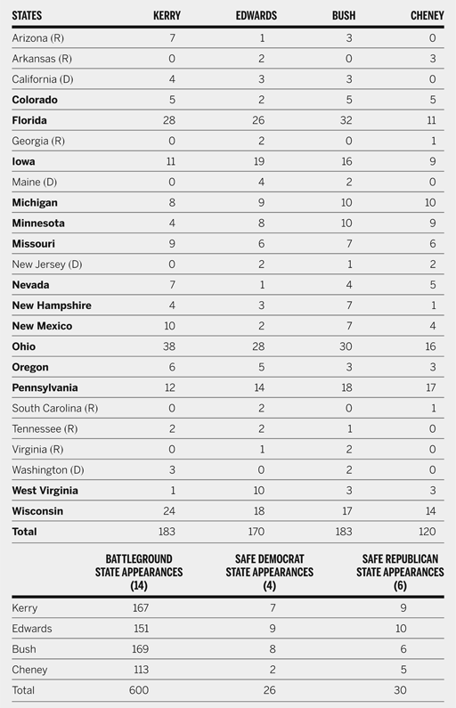
The data collected for the 2004 election included 656 appearancesFootnote 16 made by presidential candidates George W. Bush and John Kerry and their respective running mates, Richard Cheney and John Edwards, over the 14 weeks beginning in August and ending the week before the election. These appearances were distributed over 14 battleground states, six safe Republican states, and four safe Democratic states (see appendix B).
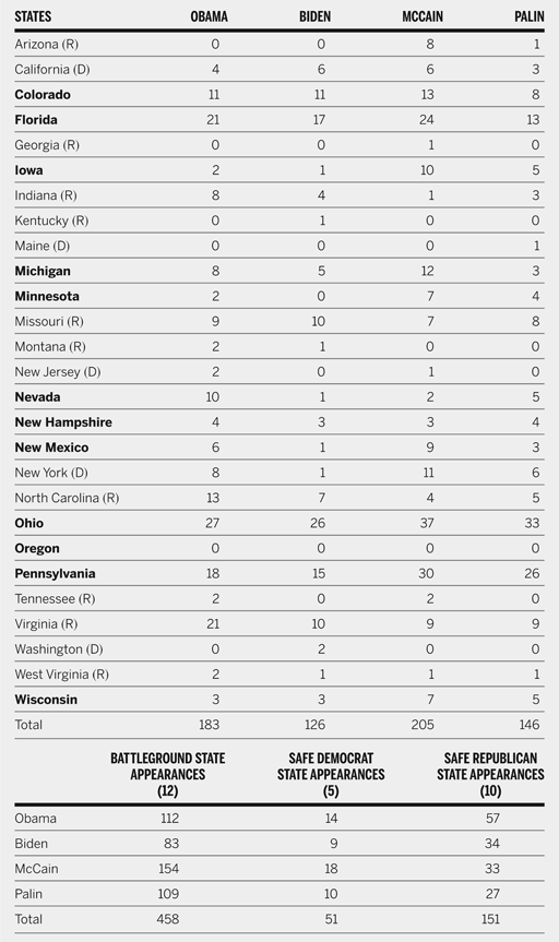
Finally, our analysis compared campaign appearances made by the 2008 presidential candidates Barack Obama and John McCain and their respective running mates, Joseph Biden and Sarah Palin. We collected data on 660 appearancesFootnote 17 made between August 4, 2008, and Election Day (November 4, 2008) spread over 12 battleground states, five safe Democratic states, and ten safe Republican states (see appendix C).
RESULTS
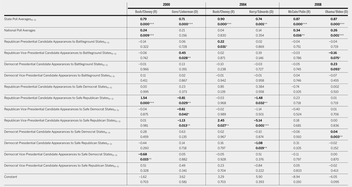
Table 1 shows the results for the six equations representing the six pairs of presidential candidates in the 2000, 2004, and 2008 campaigns.Footnote 18 For each equation, we investigated how the dependent variable, the presidential candidates' weekly state poll numbers, responded to appearances by that year's presidential and vice-presidential candidates.
Models of Presidential Campaign Appearances 2000, 2004, and 2008

* p < .10;
** p < .05;
*** p < .01
Top line = coefficient, bottom line = significance level. 2000 election: number of observations = 364, number of states = 28; Gore model, R 2 = 0.768, Wald chi2 = 730.78, p > chi2 (0.000); Bush model, R 2 = 0.8280, Wald chi2 = 529.32, p > chi2 (0.000). 2004 election: number of observations = 263, number of states = 24; Bush model, R 2 = 0.909, Wald chi2 = 717.34, p > chi2 (0.000); Kerry model, R 2 = 0.79, Wald chi2 = 226.46, p > chi2 (0.000). 2008 election, number of observations = 351, number of states = 27; Obama model, R 2 = 0.860, Wald chi2 = 911.09, p > chi2 (0.000); McCain model, R 2 = 0.80, Wald chi2 = 581.12, p > chi2 (0.000). Bold type is used to highlight significant coefficients and their accompanying probability values. We use (t−1) to indicate independent variables that have been lagged by one week. Thus, to find the impact of an appearance in week two, we look at the number of appearances that were made in the previous week.
As seen by the chi-squared statistics at the bottom of the table, each model appears to be a good fit and is highly significant. Not surprisingly, the average state polls for the previous week are significant for all six equations. National poll averages, the variable used to control for the impact of national events that were independent of a candidate's appearances, vary in significance across the candidates and elections. Interestingly, they are only significant for the 2000 Bush campaign and the campaigns of both parties' candidates in 2008.
Appearances in Battleground States
Of more relevance to our research question are the coefficients of the remaining variables. Looking at the impact of candidates' appearances in battleground states, we find virtually all of the coefficients to be insignificant. Only two coefficients are significant and in the expected direction. In 2004, an appearance by Republican George Bush increased his support by 0.22% in the following week's poll. An appearance by Barack Obama in 2008 increased his support by 0.23% in the subsequent state polls, but it is only weakly significant (p < .10). Both of these coefficients are certainly small, and we do not wish to overemphasize their importance. However, appendices B and C show that Bush made 169 trips to 14 battleground states in 2004 and Obama made 112 appearances in 12 battleground states in 2008. Some states saw few or no appearances from the candidates, while others saw as many as 32 appearances by Bush (Florida) and 27 by Obama (Ohio). Thus, while these coefficients are small, the impact of multiple appearances should be taken into account. Still, we cannot help but note the lack of significant coefficients in battleground states. We found no other significant impacts from presidential candidates. Among the vice-presidential candidates, there is only one significant coefficient consistent with our hypotheses; a weakly significant appearance (p < .10) in 2008 by Republican Sarah Palin decreased support by 0.16% for Democrat Obama.
Appearances in Non-Battleground States
Turning to non-battleground or safe states, we see that several coefficients are significant. Of interest is that (1) appearances in safe states more often work by decreasing support for an opponent rather than increasing support for the candidate, and (2) the majority of significant coefficients involve vice-presidential candidates.
Bush and Obama are the only presidential candidates whose appearances increased their support in non-battleground states. An appearance by Obama in 2008 increased his support in a safe Democratic state by a negligible 0.04%. However, in the 2000 election, an appearance by Bush in a safe Republican state increased his poll support by 1.54%. Besides increasing his own support, Bush's appearances also decreased support for his opponents. In both the 2000 and 2004 elections, an appearance by Bush in a safe Republican state decreased support for his Democratic opponents by −0.81% and −1.48%, respectively.
Looking at the vice-presidential candidates, we see only one instance in which a candidate increased support for his or her ticket, when a 2004 appearance by Republican Richard Cheney increased support for Bush by a fairly large 2.45%. That same appearance decreased support for the Democratic ticket by an even larger −5.14%. Table 1 shows that Cheney was also effective in 2000, when his appearance in a safe Republican state decreased Democratic support by −1.13% and his appearance in a safe Democratic state decreased support for the Democrats by −0.61%. Among the Democratic vice-presidential candidates, the only statistically significant coefficient is linked to Democrat Joseph Lieberman's 2000 appearance in a safe Democratic state, which decreased Republican support by −0.68%. Of the remaining vice-presidential candidates, none demonstrate a statistically significant impact in non-battleground states.
Theoretically Anomalous Coefficients
Two significant coefficients have signs that are the reverse of what we predicted. One of these involves appearances in battleground states by Republican Richard Cheney during the 2000 election. Contrary to our expectation, a battleground state appearance by Cheney appears to have increased the polling strength of the Democrats by 0.45%. In some ways, this is understandable, because Cheney was seen as a highly polarizing individual. His presence could have alienated potential Republican supporters and led them to support the Democrats. We are skeptical of this conclusion, however, because we would expect this alienation to appear in other significant coefficients involving Cheney. Yet it does not—Cheney was effective in other states. The other coefficient with a reversed sign indicates that a 2004 appearance by Democrat John Kerry actually decreased his support by −1.08% in a safe Republican state. Unlike the Cheney case, there are no other statistics showing Kerry's effectiveness in other states, and the size of the impact is relatively large. We examine this finding in the discussion.
DISCUSSION
We began our research by asking a very specific question about a particular type of campaign activity. Do candidate appearances sway voter support? Our results suggest that, yes, campaign appearances have the potential to increase voter support for a candidate and, just as important, decrease support for an opponent.
We also recognize what our results do not show. We present no evidence that appearances by a candidate changed the outcome of an election, either in one state or nationally. This outcome was not the focus of our research or part of our research design. We cannot ignore, however, that our results show that appearances have the greatest impact in safe states, where the outcome is not really in doubt and a small change does little good. In battleground states where a small shift can make a large difference, appearances had almost no effect, and the few exceptions were still small.
MINIMAL EFFECTS HYPOTHESIS REVISITED
In many ways, our results support the minimal effects hypothesis. However, one explanation of the minimal effects hypothesis is that one candidate's efforts are offset by the efforts of his or her opponent. As Shaw describes it, “the opposing campaign is likely to target its activities in the same places as you, with roughly the same volume” (Reference Shaw2006, 115). The result is that any electoral advantage from the actions of one candidate is mitigated by the responses of an opponent. Both candidates are effective, but there is no visible change in voter support.
Logically, this pattern of response and counterresponse would be particularly strong for campaign appearances in battleground states, and appendices A, B, and C show that Democrats and Republicans both make a similarly large number of appearances in these states. But this pattern is not seen to the same extent in safe states, where appearances are fewer and less likely to be countered by an opponent. We suggest that this lack of countering or offsetting explains the stronger results in non-battleground states and similarly explains the weaker results in battleground states. If a candidate appearance does have an impact, it is more likely to be seen in a safe state, where there is less chance it will be offset by an opponent's appearance, and less likely to be found in the more frequently visited battleground states. This example also explains why candidates make appearances, even though they may have no net effect. If candidates do not make an appearance, they allow their opponent the opportunity to build an advantage, and they risk losing the election as Dewey did when he did not counter Truman's more frequent appearances (see Holbrook Reference Holbrook2002).
Differences in State Type
Our previous discussion suggests that safe states and battleground states are different, and that one of the biggest differences is the way they are targeted by the candidates. Certainly there are other differences, including state demographics, that are important for understanding a party's advantage or disadvantage.Footnote 19 In addition, as we noted previously, the states can differ in how persuadable their voters are. Battleground states potentially contain a larger percentage of persuadable voters; safe states are more likely to contain larger percentages of voters responsive to appearances by one party, but not the other party.Footnote 20 These differences would account for the larger impacts (i.e., the larger coefficients) that we found in safe states. They would also explain why significant coefficients for appearances by Republicans are more likely to be found for safe Republican states, and why significant coefficients for appearances by Democrats are more likely to be found for safe Democratic states. Obviously, however, the percentage of persuadable voters is not the only factor in determining impacts in safe states. This factor may explain why there are several significant coefficients for Republican appearances in safe Republican state, but it does not explain why there is only one significant coefficient for Democratic appearances in safe Democratic states (Lieberman in 2000), and it certainly does not account for the instance of significant Republican impact from an appearance in a safe Democratic state (Cheney in 2000). To explain these differences, we need to turn to the candidates and campaigns themselves.
Interpreting Candidate Effectiveness
Judging the effectiveness of appearances by the size and significance of the coefficients in our models shows that some candidates were more effective than others, and no candidate was always effective. Even if we limit judgments to the conditions in which appearances did have an impact, we see a surprising range of differences. Among presidential candidates, George W. Bush was the most effective. Barack Obama also showed some ability to increase his support with an appearance. But appearances by Al Gore and John McCain seemed to have no effect, and some of John Kerry's appearances seemed to decrease his support.
In the campaigns we studied, the most effective appearances by any candidate were made by vice-presidential candidates. Our results could further be interpreted to suggest that Republican vice-presidential candidates were more effective than their Democratic counterparts. This interpretation, however, merely reflects the effectiveness of Richard Cheney, arguably the most effective of all of the candidates. Not all Republicans were as successful. Republican Sarah Palin did not come close to Cheney's level of impact. Nor was success limited to Republicans, given that Democrat Joseph Lieberman was also effective. Appearances by the remaining vice-presidential candidates, Democrats John Edwards and Joseph Biden, did not appear to make a difference.
Our analysis thus provides evidence that counters recent conjectures that vice-presidential selection does not matter. We recognize that there may be multiple criteria for choosing a running mate, but the ability to campaign is an important consideration that should not be overlooked.
While important, a candidate's skill in campaigning is not the only factor that determines the effectiveness of an appearance. Also important is the manner or style in which a candidate presents himself or herself (presentation of self),Footnote 21 the role that the candidate plays in a campaign, and the message that the candidate and the campaign present. A skilled candidate, given a poor message or an inappropriate role, will have the same lack of impact as an unskilled candidate. Thus, the effectiveness of some vice-presidential candidates no doubt reflects their skill, but it also reflects a fit between their skill and the decision for the vice-presidential candidate to play a more aggressive role in the campaign.
Campaign choices, rather than the skill of the candidate, could help explain the negative impact of John Kerry's appearances in safe Republican states. Although our results suggest that Kerry was not particularly effective, this negative impact is not likely to derive from former supporters who became disillusioned after hearing the candidate and left the rally shaking their heads in disgust. More likely, the impact results from choices by the campaign. Sending Kerry to a hostile (safe Republican) state possibly served to mobilize the opposition, leading to the drop in support. An alternative explanation is that Kerry was sent as a response to recent Republican gains. If so, then the apparent decline in polls may not be a result of his appearance, but may indicate that his appearance was insufficient to stop the trend.Footnote 22 In both possibilities, the decision to send the candidate represented a poor choice or a poor use of the candidate's skills.
Equally important for interpreting our results is the idea that the success of appearances will be affected by the goals and strategy of the campaign. We have been looking at the persuasive impact of campaign appearances—that is, the candidates' ability to change public opinion. But campaign appearances can also be used to mobilize supporters. For example, in 2004, Bush rallies did not try to change the mind of the unsure voter. Undecided or Democratic voters were discouraged from attending these events. Instead, Bush packed “audiences with supporters … whipping them into brigades ready to blitz crucial districts to get every last voter to the polls” (Halbfinger Reference Halbfinger2004). Similarly, in 2008, Sarah Palin accompanied John McCain in 54% of their campaign appearances. By contrast, Obama and Biden appeared together only 29% of the time. Palin's role was to attract national attention and rally the base of the party. Persuasion was secondary. Ironically, even when the strategy focused on mobilizing the base, Bush's appearances still showed the potential to persuade, whereas Palin's appearances did not significantly impact McCain's support.
In conclusion, our study examines the persuasive potential of campaign appearances. It is not an analysis of the impact of campaigns on electoral outcomes. We recognize that there are other uses of appearances, and that appearances are only one part of a campaign. Candidate campaign appearances are, however, an important factor that has the potential to shift public opinion. The results of our study are subtle, in part because of the offsetting actions of both campaigns, and in part because the appearance is simply a part of the campaign process. Beyond the direct impact on people who attend a candidate's event, appearances also have an effect on other voters. In a sense, campaign appearances are similar to a rock being thrown into a pond. There is the initial splash as the rock hits the water, and then ripples spread out to all edges of the pond.Footnote 23 The splash is certainly important, but our analysis shows that we also need to study the ripples.
APPENDIX A
Presidential and Vice Presidential Candidate Appearances to Battleground and Non-Battleground States, August 7 to November 7, 2000

Source: 2000 database provided by Democracy in Action, George Washington University; and LexisNexis database. Battleground states are indicated by bold type. Safe Democratic states are followed by a (D) and safe Republican states are followed by an (R).
APPENDIX B
Presidential and Vice Presidential Candidate Appearances to Battleground and Non-Battleground States, August 2 to November 2, 2004

Source: Democracy in Action, George Washington University; LexisNexis Academic; CNN Elections 2004; Timewatch.org; Chicago Tribune Elections; PBS Vote 2004; C-SPAN Elections. Battleground states are indicated by bold type. Safe Democratic states are followed by a (D) and safe Republican states are followed by an (R).
APPENDIX C
Presidential and Vice Presidential Candidate Appearances to Battleground and Non-Battleground States, August 4 to November 4, 2008

Source: Democracy in Action, George Washington University; LexisNexis Academic; CNN Elections 2008; The New York Times, The Washington Post; C-SPAN Elections. Battleground states are indicated by bold type. Safe Democratic states are followed by a (D) and safe Republican states are followed by an (R).