1 Introduction
When open channel flow is subjected to short-wave radiative heating from above progressive absorption of radiation by the fluid leads to a volumetric heat source that decreases with depth. This, combined with turbulence generation due to shear at the solid bottom surface, leads to a non-uniform stable temperature stratification profile in which stratification and its damping effects on turbulence are strongest close to the surface and weaken with depth. This situation occurs in rivers, canals, estuaries and shallow seas under the influence of solar heating. Damping of turbulence reduces mixing of solutes in the fluid body. In the context of the environmental flows listed above, this can affect the levels and distribution of ecologically important chemical species such as dissolved oxygen, carbon dioxide, contaminants and nutrients (Turner & Erskine Reference Turner and Erskine2005).
For a given radiative forcing, the degree of turbulence damping that occurs increases as the flow rate decreases due to the associated reduction in turbulence generation due to shear at the channel bottom. Thus changes to natural flowing systems, such as the extraction of water from river systems for human purposes for example, can lead to reduced levels of dissolved oxygen along with increased contaminant concentrations, causing long-term damage to ecosystems (Turner & Erskine Reference Turner and Erskine2005). Reduced flow rates can also lead to acute ecological damage such as mass fish kills and cyanobacterial outbreaks, commonly known as algal blooms. These events have been found to be strongly associated with conditions in which high radiation levels combined with low flow rate leads to strong and persistent stable stratification (Sherman et al. Reference Sherman, Webster, Jones and Oliver1998; Webster et al. Reference Webster, Sherman, Bormans and Jones2000; Bormans, Ford & Fabbro Reference Bormans, Ford and Fabbro2005).
In previous work Williamson et al. (Reference Williamson, Armfield, Kirkpatrick and Norris2015) studied the statistically steady state reached by a turbulent open channel flow subjected to radiative heating. The radiative heating was modelled using a volumetric heat source following the Beer–Lambert law. The volumetric heat source acts as a sink of gravitational potential energy, so the equilibrium flow state represents a state in which the turbulent kinetic energy generated by shear within the channel is in global balance with a combination of viscous dissipation and this potential energy sink. Conversion of turbulent kinetic energy to potential energy occurs through a downwards buoyancy flux. This steady state flow models the situation in a physical system in which solar heating has occurred over a long enough period of time for steady state to be achieved, for example the state of a river at the end of a sunny day.
In the current paper we study the evolution of the same flow when this heat source is removed and both top and bottom boundaries are kept adiabatic. In terms of the physical analogues mentioned above, this corresponds to situations in which solar forcing is removed and there is negligible heat transfer across the upper surface and bottom. This might occur when the sky becomes cloudy or the Sun sets while air temperature and humidity remain relatively high. A study of the flow with a non-adiabatic upper surface representing convective and radiative cooling that occurs at night or as the result of the passing of a cold front is the subject of a second paper.
With no heat input the temperature field gradually mixes and stratification weakens progressively until it approaches a fully mixed isothermal state. This can again be interpreted in terms of energy transfers. In this case, however, both mean flow kinetic energy and turbulent kinetic energy are converted into potential energy. Since the potential energy sink has been removed, potential energy increases as the flow approaches a final isothermal state.
A key finding of the study by Williamson et al. (Reference Williamson, Armfield, Kirkpatrick and Norris2015) was that the turbulence in the central region of the steady state flow is in a state of local energetic equilibrium, that is
 $P\approx B+\unicode[STIX]{x1D700}$
, where
 $P$
is shear production,
 $B$
buoyancy destruction and
 $\unicode[STIX]{x1D700}$
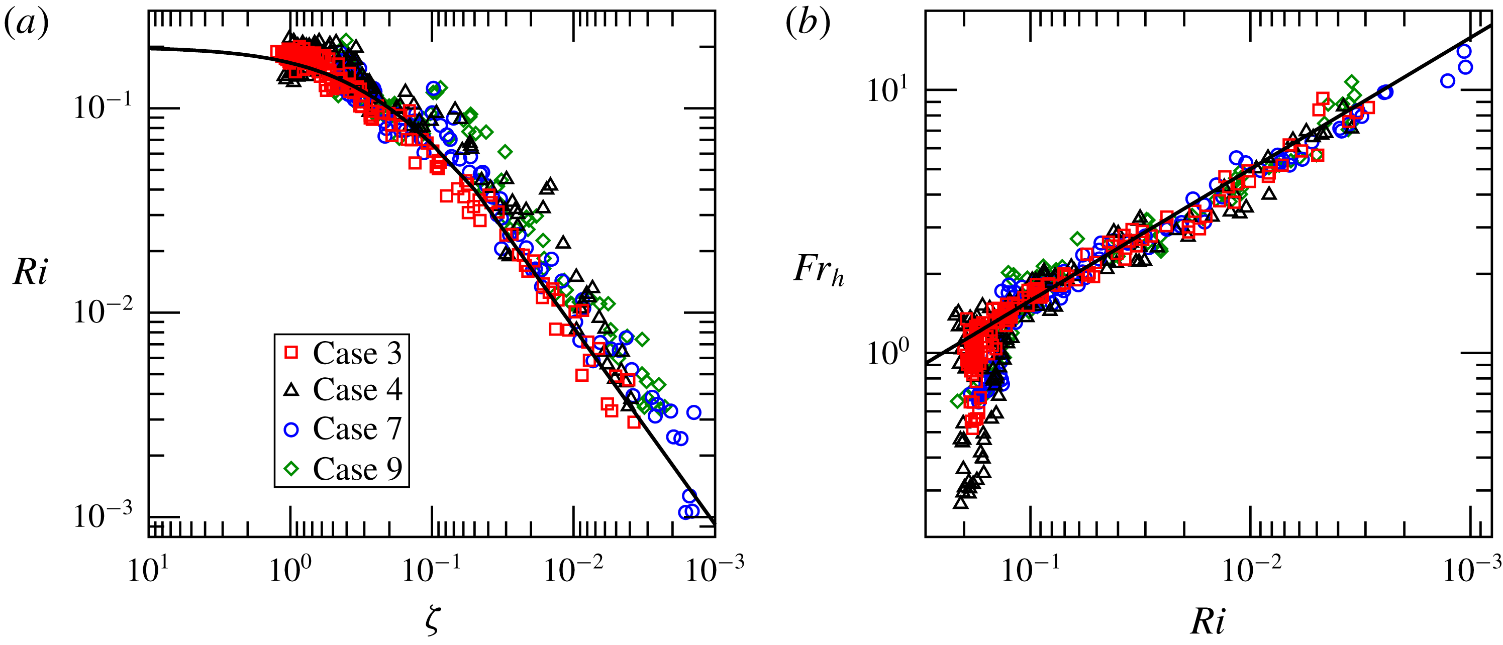
viscous dissipation of turbulent kinetic energy. As a consequence, this region exhibits behaviour similar to that seen in studies of homogeneous stratified sheared turbulence such as those of Shih et al. (Reference Shih, Koseff, Ivey and Ferziger2005) and Chung & Matheou (Reference Chung and Matheou2012). In the destratifying flow, we find that this region remains in energetic equilibrium as the flow evolves. As a consequence, as the flow destratifies, it sweeps through large ranges of local turbulence parameters such as the gradient Richardson number
 $Ri$
and buoyancy Reynolds number
 $Re_{b}$
, making it a useful flow for determining scaling relationships between these local turbulence parameters and local flow properties such as eddy diffusivity
 $k_{h}$
.
Previous studies of stratified channel flow such as those of Garg et al. (Reference Garg, Ferziger, Monismith and Koseff2000), Taylor, Sarkar & Armenio (Reference Taylor, Sarkar and Armenio2005) and Garcia-Villalba & del Alamo (Reference Garcia-Villalba and del Alamo2011) have found the friction Richardson number
 $Ri_{\unicode[STIX]{x1D70F}}$
to be a useful parameter for characterising buoyancy effects in this context. Again, our destratifying flow sweeps through a large range of this parameter allowing us to explore the relationships between
 $Ri_{\unicode[STIX]{x1D70F}}$
and local flow parameters and properties such as
 $Re_{b}$
and
 $k_{h}$
, as well as bulk flow behaviour such as the destratification rate.
Studies of the time evolution of turbulent flows due to a change in thermal forcing are relatively few in number. A recent experimental study by Van Buren et al. (Reference Van Buren, Williams and Smits2017) investigates the effect on a turbulent boundary layer of decreasing wall temperature. In their flow stratification is increasing with time, in contrast to our case where stratification decreases.
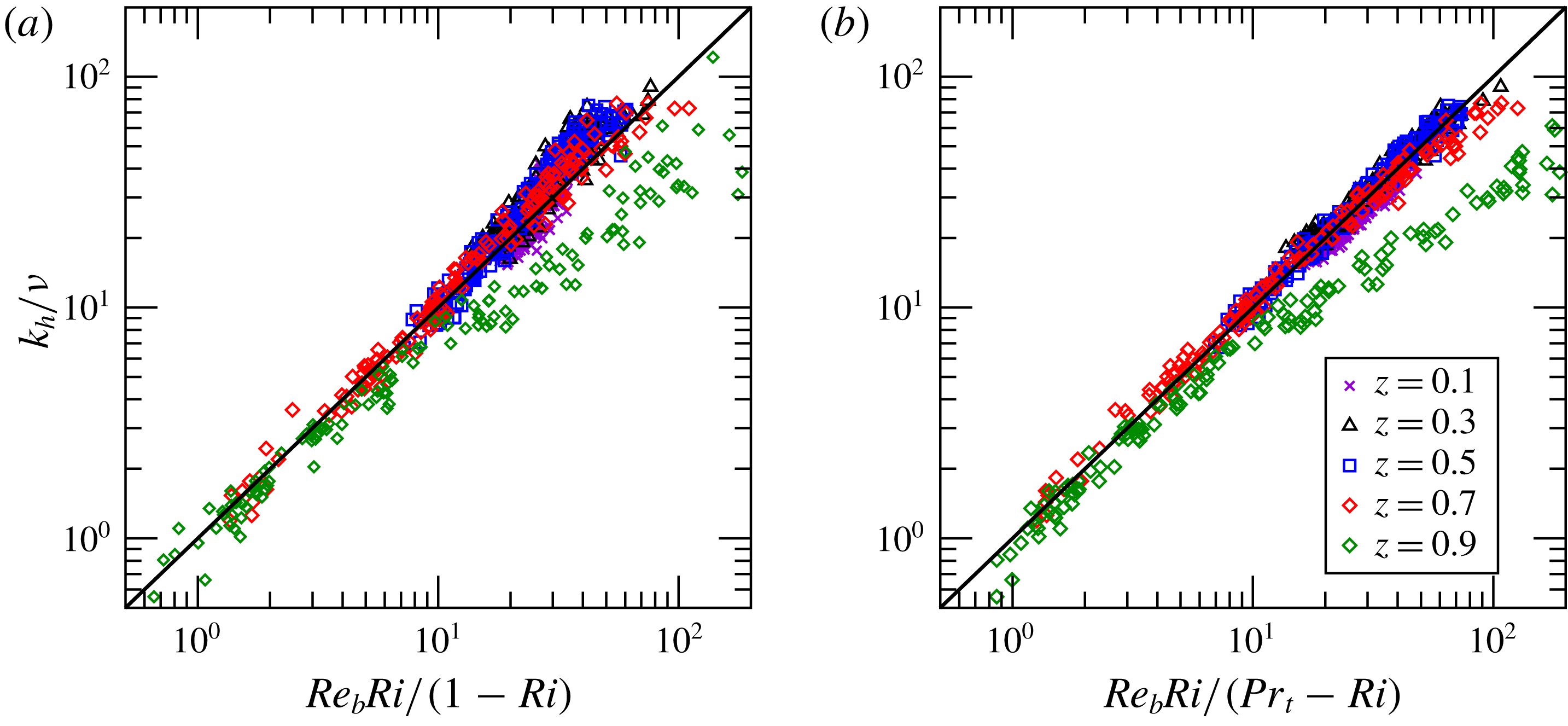
The overarching aim of this paper is to determine a scaling relationship for the destratification rate in terms of bulk parameters that can be predicted by large scale forecasting models such as hydraulic river models. Global destratification rate is dependent on vertical turbulent transport of heat within the channel, which depends on eddy diffusivity. So our approach is to first investigate relationships between eddy diffusivity
 $k_{h}$
and local turbulence parameters such as
 $Ri$
and
 $Re_{b}$
. We then extend this to include bulk parameters
 $Re_{\unicode[STIX]{x1D70F}}$
and
 $Ri_{\unicode[STIX]{x1D70F}}$
. This leads finally to a scaling relationship for destratification rate in terms of bulk parameters that is justifiable in terms of our observations regarding the physical processes occurring locally within the channel.
The remainder of this paper is structured as follows. Section 2 describes the mathematical formulation of the problem including the governing equations and non-dimensionalisation approach used. Details of the numerical simulations including the numerical methods used and the parameter ranges considered are given in § 3. In § 4 we give an overview of the flow evolution and initial conditions. Section 5 shows how vertical profiles of important local turbulence parameters change as the flow evolves. Section 6 discusses bulk flow energetics and energy transfers. Section 7 discusses relationships amongst local parameters in the central region of the channel and introduces the mixed parameter
 ${\mathcal{Q}}=Re_{b}/Re_{\unicode[STIX]{x1D70F}}$
while § 8 addresses the dynamics of the near-surface region. In § 9 we compare our data with various scalings based on Monin–Obukhov theory while § 10 discusses scalings between local turbulence parameters and the friction Richardson number
 $Ri_{\unicode[STIX]{x1D70F}}$
. Finally in § 11 we derive a scaling relationship for destratification rate in terms of bulk parameters and present results to support this model.
2 Problem formulation
2.1 The initial heated equilibrium state flow
We use the framework for the radiatively heated equilibrium state flow described by Williamson et al. (Reference Williamson, Armfield, Kirkpatrick and Norris2015). A schematic of the flow is shown in figure 1. It is an open channel flow with an adiabatic, no-slip wall at the lower surface, an adiabatic, free-slip impermeable boundary at the upper surface and periodic boundaries in the streamwise and spanwise directions. The flow is driven by a constant pressure gradient in the streamwise direction and radiative heating is represented by a depth-dependent volumetric heat source
 $\tilde{q}_{r}(\tilde{z})$
following the Beer–Lambert law,
 $$\begin{eqnarray}\tilde{q}_{r}(\tilde{z})=\tilde{I} _{s}\tilde{\unicode[STIX]{x1D6FC}}\text{e}^{(\tilde{z}-\tilde{h})\tilde{\unicode[STIX]{x1D6FC}}}.\end{eqnarray}$$
Here
 $\tilde{I} _{s}$
is the short-wave radiative heat flux through the upper surface,
 $\tilde{\unicode[STIX]{x1D6FC}}$
the attenuation coefficient due to turbidity and
 $\tilde{h}$
the channel depth. Here and throughout this paper a tilde
 $\tilde{\cdot }$
indicates a dimensional quantity, whereas a variable with no tilde is non-dimensional.
Schematic of the radiatively heated equilibrium flow.

The temperature field
 $\tilde{\unicode[STIX]{x1D719}}$
is decomposed into a time varying mean and a statistically steady fluctuating component,
 $$\begin{eqnarray}\tilde{\unicode[STIX]{x1D6F7}}(\tilde{x},\tilde{t})=\tilde{\unicode[STIX]{x1D6F7}}_{v}(\tilde{t})+\tilde{\unicode[STIX]{x1D719}}(\tilde{x},\tilde{t}).\end{eqnarray}$$
Here
 $\tilde{\unicode[STIX]{x1D6F7}}_{v}(\tilde{t})$
is the domain-averaged temperature at time
 $\tilde{t}$
, which increases with time according to
 $$\begin{eqnarray}\frac{\text{d}\tilde{\unicode[STIX]{x1D6F7}}_{v}}{\text{d}\tilde{t}}=\frac{\tilde{Q}_{r}}{\tilde{\unicode[STIX]{x1D70C}}_{b}\tilde{c}_{p}},\end{eqnarray}$$
where
 $\tilde{\unicode[STIX]{x1D70C}}_{b}$
and
 $\tilde{c}_{p}$
are a reference density and the specific heat of the fluid, and
 $\tilde{Q}_{r}$
is the domain averaged radiative heat source,
 $$\begin{eqnarray}\tilde{Q}_{r}=\frac{1}{\tilde{h}}\int _{0}^{\tilde{h}}\tilde{q}_{r}(\tilde{z})\,\text{d}\tilde{z}.\end{eqnarray}$$
The heat source is non-dimensionalised as
 $$\begin{eqnarray}q_{r}(z)=\frac{\tilde{q}_{r}(\tilde{z})-\tilde{Q}_{r}}{\tilde{Q}_{N}},\end{eqnarray}$$
where
 $$\begin{eqnarray}\tilde{Q}_{N}=\frac{1}{\tilde{h}^{2}}\int _{0}^{\tilde{h}}(\tilde{Q}_{r}-\tilde{q}_{r}(\tilde{z}))(\tilde{h}-\tilde{z})\,\text{d}\tilde{z}.\end{eqnarray}$$
The temperature fluctuation field is non-dimensionalised as
 $$\begin{eqnarray}\unicode[STIX]{x1D719}(x,t)=\frac{\tilde{\unicode[STIX]{x1D6F7}}(\tilde{x},\tilde{t})-\tilde{\unicode[STIX]{x1D6F7}}_{v}(\tilde{t})}{\tilde{\unicode[STIX]{x1D6F7}}_{N}},\end{eqnarray}$$
where
 $$\begin{eqnarray}\tilde{\unicode[STIX]{x1D6F7}}_{N}=\frac{\tilde{Q}_{N}\tilde{h}}{\tilde{\unicode[STIX]{x1D70C}}_{b}\tilde{c}_{p}\tilde{u} _{\unicode[STIX]{x1D70F}}}.\end{eqnarray}$$
Here
 $\tilde{u} _{\unicode[STIX]{x1D70F}}$
is the friction velocity associated with the shear stress on the lower solid surface.
Williamson et al. (Reference Williamson, Armfield, Kirkpatrick and Norris2015) define a non-dimensional bulk stability parameter,
 $$\begin{eqnarray}\unicode[STIX]{x1D706}=\tilde{h}/\tilde{{\mathcal{L}}},\end{eqnarray}$$
where
 $\tilde{{\mathcal{L}}}$
is a bulk Obukhov length scale defined as
 $$\begin{eqnarray}\tilde{{\mathcal{L}}}=\frac{\tilde{u} _{\unicode[STIX]{x1D70F}}^{3}}{\tilde{g}\tilde{\unicode[STIX]{x1D6FD}}\tilde{I} _{s}/\tilde{\unicode[STIX]{x1D70C}}_{b}\tilde{c}_{p}}\left(\frac{1}{2}-\frac{1}{\tilde{\unicode[STIX]{x1D6FC}}\tilde{h}}\right)^{-1}.\end{eqnarray}$$
Here
 $\tilde{g}$
is gravitational acceleration and
 $\tilde{\unicode[STIX]{x1D6FD}}$
the coefficient of thermal expansion, which relates fluid density
 $\tilde{\unicode[STIX]{x1D70C}}$
to temperature through
 $\text{d}\tilde{\unicode[STIX]{x1D70C}}/\tilde{\unicode[STIX]{x1D70C}}_{b}=-\tilde{\unicode[STIX]{x1D6FD}}\,\text{d}\tilde{\unicode[STIX]{x1D719}}$
. This formulation of the Obukhov length scale results from the current context in which the heat flux into the domain takes the form of a volumetric heat source given in (2.1), which leads to
 $$\begin{eqnarray}\tilde{Q}_{N}\approx \frac{\tilde{I} _{s}}{\tilde{h}}\left(\frac{1}{2}-\frac{1}{\tilde{\unicode[STIX]{x1D6FC}}\tilde{h}}\right).\end{eqnarray}$$
Combining this with (2.8) gives an alternative expression for
 $\unicode[STIX]{x1D706}$
,
 $$\begin{eqnarray}\unicode[STIX]{x1D706}=\frac{\tilde{\unicode[STIX]{x1D6FD}}\tilde{g}\tilde{\unicode[STIX]{x1D6F7}}_{N}\tilde{h}}{\tilde{u} _{\unicode[STIX]{x1D70F}}^{2}},\end{eqnarray}$$
which has the same form as a friction Richardson number.
The heated equilibrium state flow is governed by the Oberbeck–Boussinesq form of the equations for conservation of mass, momentum and energy for an incompressible fluid. These are written in non-dimensional Cartesian tensor form as
 $$\begin{eqnarray}\displaystyle & \displaystyle \frac{\unicode[STIX]{x2202}u_{j}}{\unicode[STIX]{x2202}x_{j}}=0, & \displaystyle\end{eqnarray}$$
 $$\begin{eqnarray}\displaystyle & \displaystyle \frac{\unicode[STIX]{x2202}u_{i}}{\unicode[STIX]{x2202}t}+\frac{\unicode[STIX]{x2202}u_{i}u_{j}}{\unicode[STIX]{x2202}x_{j}}=-\frac{\unicode[STIX]{x2202}p}{\unicode[STIX]{x2202}x_{i}}+\unicode[STIX]{x1D708}\frac{\unicode[STIX]{x2202}^{2}u_{i}}{\unicode[STIX]{x2202}x_{j}^{2}}+\unicode[STIX]{x1D6FF}_{i1}+\unicode[STIX]{x1D706}_{0}\unicode[STIX]{x1D719}\unicode[STIX]{x1D6FF}_{i3}, & \displaystyle\end{eqnarray}$$
 $$\begin{eqnarray}\displaystyle & \displaystyle \frac{\unicode[STIX]{x2202}\unicode[STIX]{x1D719}}{\unicode[STIX]{x2202}t}+\frac{\unicode[STIX]{x2202}\unicode[STIX]{x1D719}u_{j}}{\unicode[STIX]{x2202}x_{j}}=\unicode[STIX]{x1D70E}\frac{\unicode[STIX]{x2202}^{2}\unicode[STIX]{x1D719}}{\unicode[STIX]{x2202}x_{j}^{2}}+q_{r}. & \displaystyle\end{eqnarray}$$
Here
 $u_{i}$
are the Cartesian components of the velocity vector
 $\boldsymbol{u}$
,
 $p$
the pressure,
 $x_{i}$
the components of the position vector
 $\boldsymbol{x}$
,
 $t$
time,
 $\unicode[STIX]{x1D708}$
kinematic viscosity and
 $\unicode[STIX]{x1D70E}$
thermal diffusivity;
 $\unicode[STIX]{x1D6FF}_{ij}$
represents the Kronecker delta. Summation over repeated indices is assumed. The flow is driven by a constant uniform pressure gradient,
 $\unicode[STIX]{x1D6FF}_{i1}$
, in the streamwise direction;
 $q_{r}$
is the radiative volumetric heat source given in (2.1) and (2.5).
The variables are non-dimensionalised using the following scheme,
 $$\begin{eqnarray}\left.\begin{array}{@{}c@{}}\displaystyle u=\frac{\tilde{u} }{\tilde{u} _{\unicode[STIX]{x1D70F},0}},\quad \unicode[STIX]{x1D719}=\frac{\tilde{\unicode[STIX]{x1D719}}}{\tilde{\unicode[STIX]{x1D6F7}}_{N,0}},\quad p=\frac{\tilde{p}}{\tilde{\unicode[STIX]{x1D70C}}_{b}\tilde{u} _{\unicode[STIX]{x1D70F},0}^{2}},\quad x=\frac{\tilde{x}}{\tilde{h}_{0}},\quad t=\frac{\tilde{u} _{\unicode[STIX]{x1D70F},0}\tilde{t}}{\tilde{h}_{0}},\\ \displaystyle \unicode[STIX]{x1D708}=\frac{\tilde{\unicode[STIX]{x1D708}}}{\tilde{u} _{\unicode[STIX]{x1D70F},0}\tilde{h}_{0}}\equiv \frac{1}{Re_{\unicode[STIX]{x1D70F},0}},\quad \unicode[STIX]{x1D70E}=\frac{\tilde{\unicode[STIX]{x1D70E}}}{\tilde{u} _{\unicode[STIX]{x1D70F},0}\tilde{h}_{0}}\equiv \frac{1}{Re_{\unicode[STIX]{x1D70F},0}Pr}.\end{array}\right\}\end{eqnarray}$$
The subscript 0 indicates use of the characteristic length, velocity and temperature scales for the equilibrium state, that is
 $\tilde{h}_{0}$
,
 $\tilde{u} _{\unicode[STIX]{x1D70F},0}$
and
 $\tilde{\unicode[STIX]{x1D6F7}}_{N,0}$
, respectively. This distinction is necessary because in the subsequent destratifying flow the length scale
 $\tilde{h}$
and velocity scale
 $\tilde{u} _{\unicode[STIX]{x1D70F}}$
will typically vary with time.
Hence, for the equilibrium state, the friction Reynolds number is
 $$\begin{eqnarray}Re_{\unicode[STIX]{x1D70F},0}=\frac{\tilde{u} _{\unicode[STIX]{x1D70F},0}\tilde{h}_{0}}{\tilde{\unicode[STIX]{x1D708}}},\end{eqnarray}$$
the molecular Prandtl number,
 $$\begin{eqnarray}Pr=\frac{\tilde{\unicode[STIX]{x1D708}}}{\tilde{\unicode[STIX]{x1D70E}}},\end{eqnarray}$$
the stability parameter,
 $$\begin{eqnarray}\unicode[STIX]{x1D706}_{0}=\frac{\tilde{\unicode[STIX]{x1D6FD}}\tilde{g}\tilde{\unicode[STIX]{x1D6F7}}_{N,0}\tilde{h}}{\tilde{u} _{\unicode[STIX]{x1D70F},0}^{2}},\end{eqnarray}$$
and the characteristic temperature scale,
 $$\begin{eqnarray}\tilde{\unicode[STIX]{x1D6F7}}_{N,0}=\frac{\tilde{Q}_{N,0}\tilde{h}_{0}}{\tilde{\unicode[STIX]{x1D70C}}_{b}\tilde{c}_{p}\tilde{u} _{\unicode[STIX]{x1D70F},0}}.\end{eqnarray}$$
Boundary conditions for the bottom (
 $z=0$
) and top (
 $z=1$
) boundaries are
 $$\begin{eqnarray}z=0:u=v=w=0;\quad \frac{\unicode[STIX]{x2202}\unicode[STIX]{x1D719}}{\unicode[STIX]{x2202}z}=0,\end{eqnarray}$$
 $$\begin{eqnarray}z=1:\frac{\unicode[STIX]{x2202}u}{\unicode[STIX]{x2202}z}=\frac{\unicode[STIX]{x2202}v}{\unicode[STIX]{x2202}z}=0;\quad w=0;\quad \frac{\unicode[STIX]{x2202}\unicode[STIX]{x1D719}}{\unicode[STIX]{x2202}z}=0.\end{eqnarray}$$
Boundary conditions for all lateral boundaries are periodic.
The equilibrium state flow is defined by specifying
 $Re_{\unicode[STIX]{x1D70F},0}$
,
 $\unicode[STIX]{x1D706}_{0}$
,
 $Pr$
and a non-dimensional turbidity parameter
 $\unicode[STIX]{x1D6FC}_{0}=\tilde{\unicode[STIX]{x1D6FC}}\tilde{h}_{0}$
.
A random realisation of the equilibrium state flow is used as the initial conditions of the destratifying flow.
2.2 The destratifying flow
When a physical open channel flow evolves from an initially stratified state to a final neutrally stratified state, changes in the balance between turbulent and laminar shear stresses within the channel lead to changes in the mean velocity profile, resulting in an increase in the coefficient of friction,
 $C_{f}=2(\tilde{u} _{\unicode[STIX]{x1D70F}}/\tilde{U} _{b})^{2}$
. Here
 $\tilde{U} _{b}$
is the bulk flow velocity. In a physical open channel flow, the flow will typically respond with a change in height and deceleration of the flow.
In our simulations the height
 $h$
is fixed and the flow is driven by a constant pressure gradient. As a result, an increase in
 $C_{f}$
leads to an increase in the friction velocity, leading to an imbalance between wall shear stress and the applied pressure gradient. Over time, this imbalance causes the flow to gradually decelerate, reducing the friction velocity, until the force balance is restored.
In order to model the physical flow, the equations for the simulations of the destratifying flow are non-dimensionalised in terms of a time varying friction velocity
 $\tilde{u} _{\unicode[STIX]{x1D70F}}(\tilde{t})$
and height
 $\tilde{h}(\tilde{t})$
. The characteristic temperature scale used is fixed at the scale of the initial equilibrium state
 $\tilde{\unicode[STIX]{x1D6F7}}_{N,0}$
. This gives governing equations
 $$\begin{eqnarray}\displaystyle & \displaystyle \frac{\unicode[STIX]{x2202}u_{j}}{\unicode[STIX]{x2202}x_{j}}=0, & \displaystyle\end{eqnarray}$$
 $$\begin{eqnarray}\displaystyle & \displaystyle \frac{\unicode[STIX]{x2202}u_{i}}{\unicode[STIX]{x2202}t}+\frac{\unicode[STIX]{x2202}u_{i}u_{j}}{\unicode[STIX]{x2202}x_{j}}=-\frac{\unicode[STIX]{x2202}p}{\unicode[STIX]{x2202}x_{i}}+\unicode[STIX]{x1D708}\frac{\unicode[STIX]{x2202}^{2}u_{i}}{\unicode[STIX]{x2202}x_{j}^{2}}+\unicode[STIX]{x1D6FF}_{i1}+\unicode[STIX]{x1D6FE}\unicode[STIX]{x1D719}\unicode[STIX]{x1D6FF}_{i3}, & \displaystyle\end{eqnarray}$$
 $$\begin{eqnarray}\displaystyle & \displaystyle \frac{\unicode[STIX]{x2202}\unicode[STIX]{x1D719}}{\unicode[STIX]{x2202}t}+\frac{\unicode[STIX]{x2202}\unicode[STIX]{x1D719}u_{j}}{\unicode[STIX]{x2202}x_{j}}=\unicode[STIX]{x1D70E}\frac{\unicode[STIX]{x2202}^{2}\unicode[STIX]{x1D719}}{\unicode[STIX]{x2202}x_{j}^{2}}, & \displaystyle\end{eqnarray}$$
where
 $$\begin{eqnarray}\left.\begin{array}{@{}c@{}}\displaystyle u=\frac{\tilde{u} }{\tilde{u} _{\unicode[STIX]{x1D70F}}},\quad \unicode[STIX]{x1D719}=\frac{\tilde{\unicode[STIX]{x1D719}}}{\tilde{\unicode[STIX]{x1D6F7}}_{N,0}},\quad p=\frac{\tilde{p}}{\tilde{\unicode[STIX]{x1D70C}}_{b}\tilde{u} _{\unicode[STIX]{x1D70F}}^{2}},\quad x=\frac{\tilde{x}}{\tilde{h}},\quad \unicode[STIX]{x2202}t=\frac{\tilde{u} _{\unicode[STIX]{x1D70F}}\unicode[STIX]{x2202}\tilde{t}}{\tilde{h}},\quad \hat{t}=\frac{\tilde{u} _{\unicode[STIX]{x1D70F},0}\tilde{t}}{\tilde{h}_{0}},\\ \displaystyle \unicode[STIX]{x1D708}=\frac{\tilde{\unicode[STIX]{x1D708}}}{\tilde{u} _{\unicode[STIX]{x1D70F}}\tilde{h}}\equiv \frac{1}{Re_{\unicode[STIX]{x1D70F}}},\quad \unicode[STIX]{x1D70E}=\frac{\tilde{\unicode[STIX]{x1D70E}}}{\tilde{u} _{\unicode[STIX]{x1D70F}}\tilde{h}}\equiv \frac{1}{Re_{\unicode[STIX]{x1D70F}}Pr},\quad \unicode[STIX]{x1D6FE}=\frac{\tilde{\unicode[STIX]{x1D6FD}}\tilde{g}\tilde{\unicode[STIX]{x1D6F7}}_{N,0}\tilde{h}}{\tilde{u} _{\unicode[STIX]{x1D70F}}^{2}}.\end{array}\right\}\end{eqnarray}$$
The boundary conditions are the same as those for the equilibrium state flow.
Due to the time variation of the velocity and length scales used to non-dimensionalise (2.23)–(2.25), integrating them in time is problematic. Instead, we have chosen to solve a dynamically equivalent set of equations and then renormalise the solution to give the solution to the equations above. This procedure is described in appendix A.
Whilst (2.23)–(2.25) were not solved directly, they are useful in the context of scaling analysis because they give the time rate of change of the dependent variables,
 $\boldsymbol{u}$
,
 $p$
and
 $\unicode[STIX]{x1D719}$
, relative to a characteristic friction time scale
 $\tilde{t}_{\unicode[STIX]{x1D70F}}=\tilde{h}/\tilde{u} _{\unicode[STIX]{x1D70F}}$
determined from flow conditions at a particular instant in ‘measured time’,
 $\hat{t}$
. In our simulations, measured time,
 $\hat{t}$
, is dimensional time
 $\tilde{t}$
normalised in terms of the initial friction velocity and height as shown in (2.26). Thus, in the following,
 $t$
is used only within differentials
 $\unicode[STIX]{x2202}t$
and
 $\text{d}t$
, while
 $\hat{t}$
refers to the point in time within the process at which a particular set of flow conditions occur.
In place of the stability parameter
 $\unicode[STIX]{x1D706}_{0}$
, the buoyancy term of the momentum equations for the destratifying flow (2.24) uses
 $\unicode[STIX]{x1D6FE}$
, which is defined as
 $$\begin{eqnarray}\unicode[STIX]{x1D6FE}=\frac{\tilde{\unicode[STIX]{x1D6FD}}\tilde{g}\tilde{\unicode[STIX]{x1D6F7}}_{N,0}\tilde{h}}{\tilde{u} _{\unicode[STIX]{x1D70F}}^{2}}.\end{eqnarray}$$
In the destratifying flow,
 $\unicode[STIX]{x1D706}_{0}$
no longer has the same function as it does in the equilibrium state equations. In the equilibrium state equations,
 $\unicode[STIX]{x1D706}_{0}$
, through its dependence on
 $Q_{N}$
, couples the heat source
 $q_{r}$
in the temperature equation to the buoyancy term
 $\unicode[STIX]{x1D706}_{0}\unicode[STIX]{x1D719}$
in the momentum equations. At the same time it is also a function of the wall shear stress via friction velocity
 $\tilde{u} _{\unicode[STIX]{x1D70F},0}$
. Through these interconnections it determines the stability of the equilibrium state flow. In the transient flow simulations this coupling no longer exists since
 $q_{r}$
has been removed and
 $\unicode[STIX]{x1D719}$
is normalised by
 $\tilde{\unicode[STIX]{x1D6F7}}_{N,0}$
frozen at its equilibrium state value.
Like
 $\unicode[STIX]{x1D706}$
,
 $\unicode[STIX]{x1D6FE}$
also has a form similar to the friction Richardson number,
 $$\begin{eqnarray}Ri_{\unicode[STIX]{x1D70F}}=\frac{\tilde{\unicode[STIX]{x1D6FD}}\tilde{g}\unicode[STIX]{x0394}\tilde{\unicode[STIX]{x1D719}}\tilde{h}}{\tilde{u} _{\unicode[STIX]{x1D70F}}^{2}},\end{eqnarray}$$
where
 $\unicode[STIX]{x0394}\tilde{\unicode[STIX]{x1D719}}$
is the difference between the mean temperature at the top and bottom of the channel.
 $Ri_{\unicode[STIX]{x1D70F}}$
can be reformulated in terms of our non-dimensional variables as
 $$\begin{eqnarray}Ri_{\unicode[STIX]{x1D70F}}=\frac{\unicode[STIX]{x1D6FE}\unicode[STIX]{x0394}\unicode[STIX]{x1D719}h}{u_{\unicode[STIX]{x1D70F}}^{2}}.\end{eqnarray}$$
The friction Richardson number
 $Ri_{\unicode[STIX]{x1D70F}}$
is a bulk parameter that represents the ratio between stabilising effects of temperature stratification and the destabilising effects of shear at the wall. At high
 $Ri_{\unicode[STIX]{x1D70F}}$
the effects of temperature stratification are dominant and the flow is strongly affected by buoyancy. At low
 $Ri_{\unicode[STIX]{x1D70F}}$
the effect of shear dominates and the flow is only weakly affected by buoyancy. The destratification process involves moving from an initial state in which the flow is strongly affected by buoyancy to a final state in which buoyancy effects are insignificant.
The parameter
 $Ri_{\unicode[STIX]{x1D70F}}$
has been found to be a useful bulk parameter for characterising buoyancy effects in other types of stratified channel flow (see Garg et al.
Reference Garg, Ferziger, Monismith and Koseff2000; Garcia-Villalba & del Alamo Reference Garcia-Villalba and del Alamo2011, for example). Based on this, and given that
 $\unicode[STIX]{x1D706}$
determines the stability of the heated equilibrium flow and has a form similar to
 $Ri_{\unicode[STIX]{x1D70F}}$
, we suggest that
 $Ri_{\unicode[STIX]{x1D70F}}$
plays the equivalent function in the destratifying flow.
Thus the proposed governing parameters for the destratifying flow are
 $Re_{\unicode[STIX]{x1D70F}}$
,
 $Ri_{\unicode[STIX]{x1D70F}}$
,
 $Pr$
with
 $\unicode[STIX]{x1D6FC}_{0}$
and
 $\unicode[STIX]{x1D706}_{0}$
affecting the flow only via the initial conditions.
3 Numerical simulations
A set of initial states covering a range of turbulence and stability conditions was generated by running direct numerical simulations (DNS) of the heated equilibrium state flow solving (2.13)–(2.15). Equilibrium states were generated for the parameter combinations shown in table 1. Whilst we have proposed that
 $Ri_{\unicode[STIX]{x1D70F}}$
takes the place of
 $\unicode[STIX]{x1D706}_{0}$
as a governing parameter for the destratifying flow, since it is not a governing parameter for the equilibrium state flow it was not possible generate initial conditions corresponding to specific values of
 $Ri_{\unicode[STIX]{x1D70F}}$
. Instead we have varied
 $\unicode[STIX]{x1D706}_{0}$
. The initial values of the friction Richardson number
 $Ri_{\unicode[STIX]{x1D70F},0}$
are also shown.
Each simulation was run for an initial spin-up period of
 $t=0{-}30$
for the
 $\unicode[STIX]{x1D706}_{0}=0{-}1$
cases and
 $t=0{-}40$
for the
 $\unicode[STIX]{x1D706}_{0}=2$
cases. By these times bulk parameters such as wall shear stress, bulk and mean velocities and the temperature difference between the upper and lower surfaces had reached statistically steady state. Full realisations of the flow state were then recorded over a further 20 time units at an interval of 0.5 time units to allow the calculation of equilibrium state statistics where required.
Using each of these equilibrium states as the initial conditions, a set of transient simulations was run solving (2.23)–(2.25). Realisations of the transient flow were recorded at intervals of 0.1 time units. The total integration time for transient simulations depends on the initial conditions and ranged between approximately 5 and 15 time units.
As discussed above, the friction velocity increases as the flow destratifies and adapts to the changes in the turbulent shear stress profile. As a result the actual friction Reynolds number of the time evolving simulations increases. This increase is significant, especially for the high
 $\unicode[STIX]{x1D706}_{0}$
cases. The maximum Reynolds number reached in each case is shown in table 1.
Simulations were performed using the PUFFIN code (Kirkpatrick Reference Kirkpatrick2002). The equations are discretised in space using a finite volume formulation on a non-uniform, staggered, Cartesian grid. The grid is uniform in the
 $x$
and
 $y$
directions. Here, the grid cell sizes in viscous wall units are
 $\unicode[STIX]{x0394}x_{0}^{+}=\unicode[STIX]{x0394}y_{0}^{+}=2.95$
. In the
 $z$
direction the grid is stretched from
 $\unicode[STIX]{x0394}z_{0}^{+}=0.36$
at the bottom boundary, to
 $\unicode[STIX]{x0394}z_{0}^{+}=2.2$
for
 $z=0.4{-}0.8$
and then down to
 $\unicode[STIX]{x0394}z_{0}^{+}=0.9$
at the upper boundary. These values are based on the initial Reynolds number of the simulation. For
 $\unicode[STIX]{x1D706}_{0}=2$
cases, in which the friction velocity increases by approximately 20 % during the simulation, these
 $\unicode[STIX]{x1D6E5}^{+}$
values will also increase by approximately 20 %. The number of cells in each direction depends on
 $Re_{\unicode[STIX]{x1D70F},0}$
and is given in table 2.
Simulation parameters defined in terms of initial heated equilibrium state.

Grids and domain sizes used for each Reynolds number.

A domain with dimensions
 $2\unicode[STIX]{x03C0}\times \unicode[STIX]{x03C0}\times 1$
in the
 $x$
,
 $y$
and
 $z$
directions, respectively, was used for all simulations. Williamson et al. (Reference Williamson, Armfield, Kirkpatrick and Norris2015) present results for the heated equilibrium flow on domains of size up to
 $8\unicode[STIX]{x03C0}\times 4\unicode[STIX]{x03C0}\times 1$
. The differences between the results on the
 $8\unicode[STIX]{x03C0}\times 4\unicode[STIX]{x03C0}\times 1$
and
 $2\unicode[STIX]{x03C0}\times \unicode[STIX]{x03C0}\times 1$
domain for the flow parameters that will be discussed in this paper were found to be negligible.
The spatial discretisation uses fourth-order central differences for the advection terms in the momentum and energy equations. The fourth-order interpolations are computed using the scheme of Hokpunna & Manhart (Reference Hokpunna and Manhart2010). All other terms in the momentum, energy and pressure correction equations are discretised using second-order central differences. The equations are integrated in time using a second-order accurate fractional step method. The momentum and energy equations are integrated using a second-order hybrid Adams–Bashforth/Adams–Moulton scheme in which the diffusion terms are solved implicitly while all other terms are solved explicitly. Mass conservation is enforced using the pressure-correction method of van Kan (Reference van Kan1986) and Bell, Colella & Glaz (Reference Bell, Colella and Glaz1989). The time step
 $\unicode[STIX]{x0394}t$
was adjusted automatically to ensure that the maximum CFL (Courant–Friedrichs–Lewy) number
 $(\unicode[STIX]{x0394}tu_{i}/\unicode[STIX]{x0394}x_{i})$
in the domain remained in the range
 $0.18{-}0.2$
. Here
 $\unicode[STIX]{x0394}x_{i}$
is the cell width in the direction of the velocity component
 $u_{i}$
.
Resolution relative to the Kolmogorov scale
 $\unicode[STIX]{x1D702}$
can be estimated for Case 3 from the plot of Kolmogorov scale given in figure 9. For this case the grid size in the
 $x$
and
 $y$
directions is
 $\unicode[STIX]{x0394}x=\unicode[STIX]{x0394}y=5.5\times 10^{-3}$
while in the
 $z$
direction the grid varies from
 $\unicode[STIX]{x0394}z=7\times 10^{-4}$
at the bottom boundary, to
 $\unicode[STIX]{x0394}z=4\times 10^{-3}$
for
 $z=0.4{-}0.8$
and then to
 $\unicode[STIX]{x0394}z=1.7\times 10^{-3}$
at the upper boundary. Vertical profiles of the Kolmogorov scale for the equilibrium and time-evolving flows for Case 3 (figure 9) show that the minimum values of
 $\unicode[STIX]{x1D702}$
range from
 $\unicode[STIX]{x1D702}\approx 2.2\times 10^{-3}$
close to the bottom boundary to
 $\unicode[STIX]{x1D702}\approx 4\times 10^{-3}$
in the central region of the channel and
 $\unicode[STIX]{x1D702}\approx 8\times 10^{-3}$
close to the top surface. Thus the grid cell size relative to Kolmogorov scale ranges from approximately
 $\unicode[STIX]{x0394}x/\unicode[STIX]{x1D702}=\unicode[STIX]{x0394}y/\unicode[STIX]{x1D702}\approx 2$
close to the bottom boundary, to
 $\unicode[STIX]{x0394}x/\unicode[STIX]{x1D702}=\unicode[STIX]{x0394}y/\unicode[STIX]{x1D702}\approx 1.5$
in the central region and then
 $\unicode[STIX]{x0394}x/\unicode[STIX]{x1D702}=\unicode[STIX]{x0394}y/\unicode[STIX]{x1D702}\approx 0.5$
close to the upper surface. In the vertical direction
 $\unicode[STIX]{x0394}z/\unicode[STIX]{x1D702}\approx 0.3$
close to the bottom boundary,
 $\unicode[STIX]{x0394}z/\unicode[STIX]{x1D702}\approx 1$
in the central region and
 $\unicode[STIX]{x0394}z/\unicode[STIX]{x1D702}\approx 0.2$
close to the upper surface. Similar ratios apply to the other cases. Since the highest Prandtl number case uses
 $Pr=1$
, the Batchelor scale, given by
 $\unicode[STIX]{x1D706}_{B}=\unicode[STIX]{x1D702}/Pr^{1/2}\geqslant \unicode[STIX]{x1D702}$
for all cases. With our fourth-order spatial discretisation scheme and this degree of resolution the simulations are expected to resolve scales of motion of the order of the Kolmogorov and Batchelor scales.
To check the accuracy of the solutions Case 4 was rerun with Grid D which has spatial and temporal resolution one and a half times higher than that used for the remaining simulations. The increased resolution was found to have an indiscernible effect on the results indicating that the errors due to the numerical discretisation schemes with the grids used are negligible.
4 Overview of the flow evolution
Figures 2 and 3 show the time evolution of the temperature and vorticity fields for Case 3 for which
 $Re_{\unicode[STIX]{x1D70F},0}=540$
;
 $\unicode[STIX]{x1D706}_{0}=2$
;
 $Pr=0.71$
;
 $\unicode[STIX]{x1D6FC}_{0}=8$
. The temperature fields are at different scales in order to clearly show features. The vorticity field contours show the absolute value of the vorticity vector,
 $|\unicode[STIX]{x1D74E}|$
. The initial temperature state shows that the channel is weakly stratified in the lower half of the channel and becomes progressively more strongly stratified as the upper surface is approached. In the initial state the vorticity field exhibits characteristic features of turbulent channel flow up to a height of
 $z\approx 0.5$
, whereas in the region
 $z=0.5{-}0.8$
the turbulence is intermittent, and the strongly stratified region above
 $z=0.8$
is essentially laminar. As the flow evolves the turbulence in the flow becomes noticeably more energetic as the stratification breaks down and the temperature field mixes through the channel. In particular, the flow for
 $\hat{t}=1.5{-}7$
contains a large number of shear instabilities that have features, such as overturns in the temperature field and braided cat’s eyes in the vorticity field, that are qualitatively similar to Kelvin–Helmholtz instabilities (see Smyth & Moum Reference Smyth and Moum2000, for example). At the end of the flow evolution the flow returns to a less energetic state.
Evolution of the temperature field in the
 $x{-}z$
plane during the destratification process for Case 3:
 $Re_{\unicode[STIX]{x1D70F},0}=540$
;
 $\unicode[STIX]{x1D706}_{0}=2$
;
 $Pr=0.71$
;
 $\unicode[STIX]{x1D6FC}_{0}=8$
. The colour scale varies in order to highlight features. Flow is from left to right.

Evolution of the vorticity field in the
 $x-z$
plane during the destratification process for Case 3:
 $Re_{\unicode[STIX]{x1D70F},0}=540$
;
 $\unicode[STIX]{x1D706}_{0}=2$
;
 $Pr=0.71$
;
 $\unicode[STIX]{x1D6FC}_{0}=8$
. The colour scale is the same in all images. Flow is from left to right.

Equilibrium state buoyancy profiles for Cases 1–10.

Value of
 $Ri_{\unicode[STIX]{x1D70F}}$
as a function of time for Cases 1–10.

Figure 4 shows the buoyancy profiles for each of the initial equilibrium states. Here buoyancy is calculated as
 $\unicode[STIX]{x1D706}_{0}\langle \unicode[STIX]{x1D719}(z)-\unicode[STIX]{x1D719}_{b}\rangle$
, where
 $\unicode[STIX]{x1D719}_{b}$
is the temperature at the bottom of the channel and the angled brackets
 $\langle \;\cdot \;\rangle$
indicate averaging over both horizontal planes and time. Increasing the stability parameter
 $\unicode[STIX]{x1D706}_{0}$
of the equilibrium state increases the surface buoyancy directly via the presence of
 $\unicode[STIX]{x1D706}_{0}$
in
 $\unicode[STIX]{x1D706}_{0}\langle \unicode[STIX]{x1D719}-\unicode[STIX]{x1D719}_{b}\rangle$
. It is further increased indirectly due to the increased stability. In the initial equilibrium state the radiative heat source must be balanced by the combination of turbulent and molecular heat fluxes in order to maintain a steady state. As
 $\unicode[STIX]{x1D706}_{0}$
increases, the turbulent heat flux in the near-surface region decreases. As a result the vertical temperature gradient must increase in order to provide the increased molecular heat flux required to balance the radiative heat source.
Increasing Reynolds number
 $Re_{\unicode[STIX]{x1D70F},0}$
also increases the surface buoyancy. This can be understood by considering the case of constant
 $\tilde{u} _{\unicode[STIX]{x1D70F},0}$
and
 $\tilde{h}_{0}$
. In this situation increasing
 $Re_{\unicode[STIX]{x1D70F},0}$
implies decreasing molecular diffusivity. As with the indirect effect of
 $\unicode[STIX]{x1D706}_{0}$
above, a larger temperature gradient is then required in order to provide the necessary molecular heat flux. Increasing
 $Pr$
leads directly to lower molecular diffusivity, again requiring a larger temperature gradient, and hence increasing surface buoyancy and stability.
The turbidity parameter
 $\unicode[STIX]{x1D6FC}_{0}$
changes the vertical distribution of the radiative heat source. As
 $\unicode[STIX]{x1D6FC}_{0}$
increases, the absorption of radiation close to the surface increases while less radiation is absorbed in lower layers leading to a higher temperature gradient and increased stability close to the surface.
We refer the reader to Williamson et al. (Reference Williamson, Armfield, Kirkpatrick and Norris2015) for a detailed discussion of the turbulence characteristics of the heated equilibrium flow states.
After removal of the heat source the flow evolves over time from an initial stratified state toward a fully mixed state with a uniform temperature. Figure 5 shows this destratification process in the form of time series of the friction Richardson number
 $Ri_{\unicode[STIX]{x1D70F}}$
. Clearly the initial conditions affect the time required for destratification of the channel to occur, with the time required increasing as the friction Richardson number in the initial state
 $Ri_{\unicode[STIX]{x1D70F},0}$
increases. In the following sections we will discuss the effect of the initial state, determined by
 $Re_{\unicode[STIX]{x1D70F},0}$
,
 $\unicode[STIX]{x1D706}_{0}$
,
 $Pr$
and
 $\unicode[STIX]{x1D6FC}_{0}$
, as well as the governing flow parameters,
 $Re_{\unicode[STIX]{x1D70F}}$
,
 $Ri_{\unicode[STIX]{x1D70F}}$
and
 $Pr$
on the evolution of the flow during the destratification process and the resultant effects on destratification rate.
5 Vertical profiles
Vertical profiles showing the transient response of selected flow statistics for Case 3 (
 $Re_{\unicode[STIX]{x1D70F},0}=540$
;
 $\unicode[STIX]{x1D706}_{0}=2$
;
 $Pr=0.71$
;
 $\unicode[STIX]{x1D6FC}_{0}=8$
) are presented in figure 6. Statistics are shown for the initial state, and then at five times during the evolution of the flow. The times chosen correspond approximately to the flow field visualisations shown in figures 2 and 3. The statistics for the initial equilibrium state were calculated over 30 time units with realisations sampled at 0.5 time unit intervals. This was not possible for the statistics measured during the transient flow, however, in order to improve convergence of the statistics the values given in the plots were obtained by averaging over intervals of one time unit, using flow realisations sampled at intervals of 0.1 time units in addition to averaging over horizontal planes.
Panels (a,b) show
 $\langle \hat{u} \rangle$
and
 $\langle u\rangle$
, the mean streamwise velocity normalised in terms of the initial friction velocity
 $u_{\unicode[STIX]{x1D70F},0}$
, and time-varying friction velocity
 $u_{\unicode[STIX]{x1D70F}}$
respectively. The former is the velocity that is actually generated in the simulation before the results are renormalised (see appendix A). Panel (c) shows mean temperature
 $\langle \unicode[STIX]{x1D719}\rangle$
. Panels (d,e) show profiles of turbulent shear stress
 $\langle u^{\prime }w^{\prime }\rangle$
and turbulent heat flux
 $\langle \unicode[STIX]{x1D719}^{\prime }w^{\prime }\rangle$
. Panel (f) shows the non-dimensional vertical eddy diffusivity,
 $$\begin{eqnarray}k_{h}=\frac{-\langle \unicode[STIX]{x1D719}^{\prime }w^{\prime }\rangle }{\unicode[STIX]{x2202}\langle \unicode[STIX]{x1D719}\rangle /\unicode[STIX]{x2202}z},\end{eqnarray}$$
which is related to the dimensional eddy diffusivity,
 $$\begin{eqnarray}\tilde{k}_{h}=\frac{-\langle \tilde{\unicode[STIX]{x1D719}}^{\prime }\tilde{w}^{\prime }\rangle }{\unicode[STIX]{x2202}\langle \tilde{\unicode[STIX]{x1D719}}\rangle /\unicode[STIX]{x2202}\tilde{z}},\end{eqnarray}$$
through
 $$\begin{eqnarray}k_{h}=\frac{\tilde{k}_{h}}{\tilde{u} _{\unicode[STIX]{x1D70F}}\tilde{h}}.\end{eqnarray}$$
Here fluctuating quantities relative to the horizontal mean
 $\langle \;\cdot \;\rangle$
are denoted with primes, (for example
 $w^{\prime }$
and
 $\unicode[STIX]{x1D719}^{\prime }$
).
Vertical profiles showing the transient response of selected flow statistics at various times for Case 3. Here the thin dotted line corresponds to
 $k_{h}=\unicode[STIX]{x1D70E}$
, while the thin dashed line corresponds to
 $z=0.75$
.

As the flow evolves, the initial temperature stratification is broken down by turbulent mixing and viscous diffusion and the system approaches a state with a uniform mean temperature of
 $\langle \unicode[STIX]{x1D719}\rangle =0$
, corresponding to zero total potential energy. The downwards turbulent heat flux has a maximum in the range
 $z=0.5-0.7$
. This region of low turbulent heat flux divergence corresponds to the region in which the temperature remains relatively constant at
 $\langle \unicode[STIX]{x1D719}\rangle =0$
throughout the flow evolution.
In the initial state, the relatively high degree of stratification in the upper portion of the channel leads to reduced turbulent mixing in this region. This is apparent in the profiles of
 $\langle u^{\prime }w^{\prime }\rangle$
,
 $\langle \unicode[STIX]{x1D719}^{\prime }w^{\prime }\rangle$
and
 $k_{h}$
, which show a notable depression in magnitude in the near-surface region. As a result, the momentum transport required to balance the streamwise pressure gradient in this region must be provided predominantly by viscous shear, leading to a substantial increase in the mean streamwise velocity close to the surface relative to the final unstratified flow.
In the early stages of the destratification process the turbulent shear stress
 $\langle u^{\prime }w^{\prime }\rangle$
increases substantially, before gradually decreasing to the neutral flow profile. As can be seen from (a), this change in the balance between turbulent and viscous shear leads to a redistribution of velocity over the height of the channel, with the near-surface region slowing down, while the velocity close to the bottom surface increases. It is this change that leads to the increase in the coefficient of friction
 $C_{f}$
and friction velocity
 $u_{\unicode[STIX]{x1D70F}}$
. The inflected initial velocity profile implies a surplus of mean flow kinetic energy,
 $K(z,\hat{t})=1/2\langle u\rangle ^{2}(z,\hat{t})$
, in the initial flow relative to the final state.
The turbulent heat flux
 $-\langle \unicode[STIX]{x1D719}^{\prime }w^{\prime }\rangle$
also increases substantially, particularly in the upper half of the channel before gradually decreasing again as the process proceeds. As will be discussed in detail below,
 $-\langle \unicode[STIX]{x1D719}^{\prime }w^{\prime }\rangle$
provides a pathway for conversion of mean flow kinetic energy and energy due to the pressure gradient into potential energy. The eddy diffusivity
 $k_{h}$
increases substantially across the channel as the flow destratifies due to the increase in
 $-\langle \unicode[STIX]{x1D719}^{\prime }w^{\prime }\rangle$
relative to the mean temperature gradient.
Transient response of dominant terms in the turbulent kinetic energy equation for Case 3. Legend as for figure 6.

Figure 7 show the transient response of the dominant terms in the turbulent kinetic energy equation. For this flow, which is homogeneous on
 $x-y$
planes, the turbulent kinetic energy equation can be written as
 $$\begin{eqnarray}\frac{\unicode[STIX]{x2202}k}{\unicode[STIX]{x2202}t}=\frac{\unicode[STIX]{x2202}}{\unicode[STIX]{x2202}z}\left[-\frac{1}{2}\langle w^{\prime }u_{i}^{\prime }u_{i}^{\prime }\rangle -\langle w^{\prime }p^{\prime }\rangle +2\unicode[STIX]{x1D708}\langle s_{i3}u_{i}^{\prime }\rangle \right]-\langle u^{\prime }w^{\prime }\rangle \frac{\unicode[STIX]{x2202}\langle u\rangle }{\unicode[STIX]{x2202}z}+\unicode[STIX]{x1D6FE}\langle \unicode[STIX]{x1D719}^{\prime }w^{\prime }\rangle -2\unicode[STIX]{x1D708}\langle s_{ij}s_{ij}\rangle ,\end{eqnarray}$$
where turbulent kinetic energy
 $k=1/2\langle u_{i}^{\prime }u_{i}^{\prime }\rangle$
and
 $s_{ij}$
is the strain rate due to velocity fluctuations given by
 $$\begin{eqnarray}s_{ij}=\frac{1}{2}\left(\frac{\unicode[STIX]{x2202}u_{i}^{\prime }}{\unicode[STIX]{x2202}x_{j}}+\frac{\unicode[STIX]{x2202}u_{j}^{\prime }}{\unicode[STIX]{x2202}x_{i}}\right).\end{eqnarray}$$
For this flow the dominant terms are the unsteady term
 $U_{k}=\unicode[STIX]{x2202}k/\unicode[STIX]{x2202}t$
, transport due to turbulent fluctuations
 $T=-1/2\unicode[STIX]{x2202}\langle w^{\prime }u_{i}^{\prime }u_{i}^{\prime }\rangle /\unicode[STIX]{x2202}z$
, shear production
 $P=-\langle u^{\prime }w^{\prime }\rangle \unicode[STIX]{x2202}\langle u\rangle /\unicode[STIX]{x2202}z$
, downwards buoyancy flux (or buoyancy destruction)
 $B=-\unicode[STIX]{x1D6FE}\langle \unicode[STIX]{x1D719}^{\prime }w^{\prime }\rangle$
and dissipation rate
 $\unicode[STIX]{x1D700}=2\unicode[STIX]{x1D708}\langle s_{ij}s_{ij}\rangle$
. Panels (a–f) show
 $P$
,
 $\unicode[STIX]{x1D700}$
,
 $B$
,
 $T$
,
 $U_{k}$
and
 $k$
, while in (g–j) the terms
 $P$
,
 $B$
,
 $T$
and
 $U_{k}$
are presented as ratios of
 $B+\unicode[STIX]{x1D700}$
.
As discussed above, conversion of turbulent kinetic energy into potential energy occurs through the downward buoyancy flux
 $-\unicode[STIX]{x1D6FE}\langle \unicode[STIX]{x1D719}^{\prime }w^{\prime }\rangle$
or equivalently the buoyancy destruction term
 $B$
. The remainder of the turbulent kinetic energy is converted into internal energy through viscous dissipation
 $\unicode[STIX]{x1D700}$
. In a real flow this increase in internal energy can be viewed as raising the potential energy of the system (see Winters et al.
Reference Winters, Lombard, Riley and D’Asaro1995). The Oberbeck–Boussinesq form of the governing equations used for this study neglects the transfer of energy from viscous dissipation to internal energy, so there is no increase in temperature and hence
 $E_{p}$
as a result of dissipation.
In the initial state, shear production, buoyancy destruction and viscous dissipation are in balance across a region from
 $z=0.2{-}0.8$
indicating that this region is in a state of local energetic equilibrium. This balance can be seen most clearly in the profile of
 $P/(B+\unicode[STIX]{x1D700})$
which is approximately equal to one in this region implying
 $P\approx B+\unicode[STIX]{x1D700}$
.
Sudden removal of the radiative heat source, or potential energy sink, at the start of the transient simulation leads to a step change in the energy balance within the channel, resulting in a rapid increase in turbulent kinetic energy, particularly in the near-surface region, during the initial stage of the flow evolution (
 $\hat{t}=0{-}3$
). Turbulent kinetic energy then remains relatively constant at this elevated state over the period
 $\hat{t}=3{-}9.5$
before decreasing again towards neutral conditions in the late stages of the process. The rapid increase in
 $k$
during
 $\hat{t}=0{-}3$
is reflected in the profile of the unsteady term
 $U_{k}$
at
 $\hat{t}=1.5$
shown in (e), which reaches a maximum value of approximately 0.75 at this time before returning to values close to zero for the remainder of the flow evolution. As seen from the profile of
 $U_{k}/(B+\unicode[STIX]{x1D700})$
in (j), in the central region of the channel even this maximum value is small relative to other terms.
The dominant budget terms,
 $P$
,
 $\unicode[STIX]{x1D700}$
and
 $B$
, in the central and upper part of the channel also increase during the initial period (
 $\hat{t}=1.5$
) as shown in (a–c). The profile of
 $P/(B+\unicode[STIX]{x1D700})$
in (g) shows a distinct increase above the value of 1 for
 $z=0.75{-}0.9$
indicating a surplus of shear production in this region, which accounts for the significant
 $U_{k}$
at this time. This shear production can be seen as a distinct band of high vorticity in the flow field visualisations shown in figure 3. By
 $\hat{t}=3$
, local energetic equilibrium has been restored and the local equilibrium region
 $P/(B+\unicode[STIX]{x1D700})\approx 1$
has extended up to approximately
 $z=0.9$
. The region
 $z=0.2{-}0.9$
then remains in local equilibrium until
 $\hat{t}\approx 8$
(see § 8) after which the extent gradually starts to decrease as turbulent transport
 $T$
starts to dominate above
 $z=0.7$
.
Thus, when the radiative heat source is removed, the flow ‘relaxes’ rapidly into a new state in which the laminar surface layer becomes turbulent and the region of energetic equilibrium extends up close to the surface. This new state is reached very early in the destratification process (by
 $\hat{t}=3$
for Case 3). The fact that a large portion of the flow remains in local equilibrium for most of the flow evolution implies that local turbulent fluxes should be a function of global gradients in these regions. This is explored further below.
The normalised buoyancy flux
 $B/(B+\unicode[STIX]{x1D700})$
shown in figure 7(h) is equivalent to the generalised form of the flux Richardson number defined by Ivey & Imberger (Reference Ivey and Imberger1991) as
 $$\begin{eqnarray}R_{f}=B/(B+\unicode[STIX]{x1D700}).\end{eqnarray}$$
Ivey & Imberger (Reference Ivey and Imberger1991) interpret this as the ratio of the rate of conversion of turbulent kinetic energy
 $k$
into background potential energy
 $E_{b}$
, to the rate at which net mechanical energy is being made available for turbulence generation. As such it is often considered to represent the local mixing efficiency. Venayagamoorthy & Koseff (Reference Venayagamoorthy and Koseff2016) point out, however, that this definition does not correctly account for the effect of counter-gradient fluxes that occur in strongly stratified flows. An example of this can be seen in (h), which shows that
 $R_{f}$
is negative in the strongly stratified region close to the surface in the early stages of the flow evolution. When the flow is in local equilibrium,
 $R_{f}$
is equal to the standard form of the flux Richardson number, defined as the ratio of buoyancy destruction to shear production, that is
 $$\begin{eqnarray}Ri_{f}=B/P.\end{eqnarray}$$
The profiles of
 $R_{f}$
show a number of distinct regions. In the initial equilibrium state
 $R_{f}$
is approximately constant over the range
 $z=0.4{-}0.75$
, with a value
 $R_{f}\approx 0.17$
. This value of
 $R_{f}$
persists until the late stages of the flow evolution and is similar to the critical value
 $R_{f,c}\approx 0.18{-}0.2$
estimated from experimental measurements by Britter (Reference Britter1974) and the theoretically derived value of
 $R_{f,c}\sim 0.15$
determined by Ellison (Reference Ellison1957). Thus we consider
 $R_{f,c}=0.17$
to represent the critical value for our flow. In this central region, vertical turbulent motions are constrained predominantly by the buoyancy length scale,
 $l_{b}$
, so that turbulent fluxes are unaffected by height
 $z$
. This corresponds to the ‘
 $z$
-less’ scaling regime in Monin–Obukhov theory.
In the region close to the bottom wall, proximity to the solid boundary places an additional spatial constraint on turbulent motions, so that turbulent fluxes become a function of both
 $l_{b}$
and
 $z$
. This can be seen in the profiles. In the equilibrium state and for times up to
 $\hat{t}=6$
,
 $R_{f}$
decreases approximately linearly with
 $z$
for
 $z<0.4$
. For later times the region affected by
 $z$
expands upwards. As the flow destratifies,
 $l_{b}$
increases and its constraining effect on turbulent motions decreases accordingly. As a result, the region in which
 $z$
is the dominant length scale expands. (Please note that in the discussion above we have used
 $l_{b}$
to denote a generic buoyancy length scale. We will provide more precise definitions of a number of buoyancy length scales below.)
In the equilibrium state, in the region
 $z=0.75{-}0.85$
,
 $R_{f}$
increases to a peak of
 $R_{f}\approx 0.2$
. As can be seen from figure 6, this is the region where both velocity shear and temperature gradient are highest. Visualisations of the equilibrium state flow fields in (a) of figures 2 and 3 show that this region contains isolated incursions by shear instabilities resembling Kelvin–Helmholtz billows. A similar peak of
 $R_{f}\approx 0.21$
is seen in the profile at
 $\hat{t}=1.5$
. In this case it is slightly higher at
 $z=0.9$
. At this time figures 2 and 3 show the presence of an intense layer of shear instabilities for
 $z=0.75{-}0.85$
with incursions up to
 $z=0.9$
. By
 $\hat{t}=3$
the peak in
 $R_{f}$
is very small and the visualisations show vorticity extending to the upper surface of the channel, and for all later times the peak has disappeared. Winters et al. (Reference Winters, Lombard, Riley and D’Asaro1995) found that pure Kelvin–Helmholtz (K–H) instabilities lead to a significant increase in
 $R_{f}$
. Thus the peak in
 $R_{f}$
seen in the early stages of our flow can be attributed to incursions by Kelvin–Helmholtz-like instabilities occurring at the intermittency boundary between the turbulent flow in the body of the channel and laminar surface layer.
Transient response of dominant terms in the temperature variance equation for Case 3. Legend as for figure 6.

Figure 8 shows the transient response of dominant terms in the temperature variance equation for Case 3. For our flow the temperature variance equation can be written as
 $$\begin{eqnarray}\frac{\unicode[STIX]{x2202}\langle \unicode[STIX]{x1D719}^{\prime 2}\rangle }{\unicode[STIX]{x2202}t}=\frac{\unicode[STIX]{x2202}}{\unicode[STIX]{x2202}z}\left[-\langle w^{\prime }\unicode[STIX]{x1D719}^{\prime 2}\rangle +\unicode[STIX]{x1D70E}\frac{\unicode[STIX]{x2202}\langle \unicode[STIX]{x1D719}^{\prime 2}\rangle }{\unicode[STIX]{x2202}z}\right]-2\langle \unicode[STIX]{x1D719}^{\prime }w^{\prime }\rangle \frac{\unicode[STIX]{x2202}\langle \unicode[STIX]{x1D719}\rangle }{\unicode[STIX]{x2202}z}-2\unicode[STIX]{x1D70E}\left\langle \frac{\unicode[STIX]{x2202}\unicode[STIX]{x1D719}^{\prime }}{\unicode[STIX]{x2202}x_{j}}\frac{\unicode[STIX]{x2202}\unicode[STIX]{x1D719}^{\prime }}{\unicode[STIX]{x2202}x_{j}}\right\rangle .\end{eqnarray}$$
Similar to the turbulent kinetic energy equation, for this flow the dominant terms are the unsteady term
 $U_{\unicode[STIX]{x1D719}}=\unicode[STIX]{x2202}\langle \unicode[STIX]{x1D719}^{\prime 2}\rangle /\unicode[STIX]{x2202}t$
, turbulent transport
 $T_{\unicode[STIX]{x1D719}}=-\unicode[STIX]{x2202}\langle w^{\prime }\unicode[STIX]{x1D719}^{\prime 2}\rangle /\unicode[STIX]{x2202}z$
, production
 $P_{\unicode[STIX]{x1D719}}=-2\langle \unicode[STIX]{x1D719}^{\prime }w^{\prime }\rangle \unicode[STIX]{x2202}\langle \unicode[STIX]{x1D719}\rangle /\unicode[STIX]{x2202}z$
and dissipation rate
 $\unicode[STIX]{x1D712}=2\unicode[STIX]{x1D70E}\langle (\unicode[STIX]{x2202}\unicode[STIX]{x1D719}^{\prime }/\unicode[STIX]{x2202}x_{j})^{2}\rangle$
. Panels (a–e) show
 $P_{\unicode[STIX]{x1D719}}$
,
 $\unicode[STIX]{x1D712}$
,
 $T_{\unicode[STIX]{x1D719}}$
,
 $U_{\unicode[STIX]{x1D719}}$
and
 $\langle \unicode[STIX]{x1D719}^{\prime 2}\rangle$
, while in (f–h) the terms
 $P_{\unicode[STIX]{x1D719}}$
,
 $T_{\unicode[STIX]{x1D719}}$
and
 $U_{\unicode[STIX]{x1D719}}$
are presented as ratios of
 $\unicode[STIX]{x1D712}$
.
As with the turbulent kinetic energy, a rapid increase in temperature variance
 $\langle \unicode[STIX]{x1D719}^{\prime 2}\rangle$
is seen during the initial stage (
 $\hat{t}=0{-}3$
) particularly in the near-surface region as this region transitions from a laminar to a turbulent state. This is reflected in a region of positive
 $U_{\unicode[STIX]{x1D719}}$
in the upper half of the channel at
 $\hat{t}=1.5$
. This burst of activity is short-lived, however, with the peak
 $\langle \unicode[STIX]{x1D719}^{\prime 2}\rangle$
decreasing substantially by
 $\hat{t}=3$
and a corresponding negative
 $U_{\unicode[STIX]{x1D719}}$
at this time. After
 $\hat{t}=3$
the temperature variance decreases progressively until it is essentially zero at the end of the destratification process. Unlike turbulent kinetic energy, with adiabatic boundaries and no internal heat source, the only source of production of temperature variance is the internal temperature gradient. As the flow destratifies this temperature gradient decays leading to a decay in the production term
 $P_{\unicode[STIX]{x1D719}}$
. Throughout the process there is turbulent transport
 $T_{\unicode[STIX]{x1D719}}$
out of the central region of the channel and into the near-wall and near-surface regions.
During the period up to
 $\hat{t}=9.5$
the production and dissipation terms remain in balance so that
 $P_{\unicode[STIX]{x1D719}}/\unicode[STIX]{x1D712}\approx 1$
over the region
 $z=0.25{-}0.9$
, similar to that seen for the turbulent kinetic energy budget terms. This is somewhat surprising considering the decay in
 $\langle \unicode[STIX]{x1D719}^{\prime 2}\rangle$
; however,
 $P_{\unicode[STIX]{x1D719}}$
and
 $\unicode[STIX]{x1D712}$
remain large in comparison with
 $T_{\unicode[STIX]{x1D719}}$
and
 $U_{\unicode[STIX]{x1D719}}$
during this period so the decay in
 $\langle \unicode[STIX]{x1D719}^{\prime 2}\rangle$
is due to a relatively small difference in two large terms. In the late stages of the process this local equilibrium is lost as dissipation exceeds production,
 $\unicode[STIX]{x1D712}>P_{\unicode[STIX]{x1D719}}$
.
Transient response of turbulent length scales and related parameters for Case 3. Legend as for figure 6. (d) The thin dashed lines correspond to
 $Ri=0.18$
and
 $Ri=1/4$
. (e) The thin dashed line corresponds to
 $Re_{S}=1$
. (f) The thin dashed line corresponds to
 $Re_{b}=5$
, while the two thin dotted lines correspond to
 $Re_{b}=7$
and
 $Re_{b}=100$
. The thin dot-dashed lines (d–f) correspond to
 $z=0.76$
and
 $z=0.86$
.

Figure 9 shows profiles of turbulence length scales and some non-dimensional parameters that can be written in terms of these length scales. Panels (a–c) show: the Kolmogorov scale
 $\unicode[STIX]{x1D702}$
, the Corrsin scale
 $l_{C}$
, and the Ozmidov scale
 $l_{O}$
, which are defined as
 $$\begin{eqnarray}\unicode[STIX]{x1D702}=\left(\frac{\unicode[STIX]{x1D708}^{3}}{\unicode[STIX]{x1D700}}\right)^{1/4},\quad l_{C}=\left(\frac{\unicode[STIX]{x1D700}}{S^{3}}\right)^{1/2},\quad l_{O}=\left(\frac{\unicode[STIX]{x1D700}}{N^{3}}\right)^{1/2}.\end{eqnarray}$$
The Kolmogorov scale characterises the smallest scales of turbulence, while the Corrsin scale is indicative of the scale above which turbulence is affected by background shear, and the Ozmidov scale, the scale above which turbulence is affected by buoyancy.
Panel (d) shows the gradient Richardson number
 $$\begin{eqnarray}Ri=N^{2}/S^{2},\end{eqnarray}$$
where the buoyancy frequency
 $N$
is given by
 $N^{2}=\unicode[STIX]{x1D6FE}\unicode[STIX]{x2202}\langle \unicode[STIX]{x1D719}\rangle /\unicode[STIX]{x2202}z$
, and mean vertical shear,
 $S=\unicode[STIX]{x2202}\langle u\rangle /\unicode[STIX]{x2202}z$
. Panel (e) shows the shear Reynolds number (see Chung & Matheou Reference Chung and Matheou2012),
 $$\begin{eqnarray}Re_{S}=\frac{\unicode[STIX]{x1D700}}{\unicode[STIX]{x1D708}S^{2}},\end{eqnarray}$$
and panel (f) the local buoyancy Reynolds number (see Gargett, Osborn & Nasmyth Reference Gargett, Osborn and Nasmyth1984; Smyth & Moum Reference Smyth and Moum2000),
 $$\begin{eqnarray}Re_{b}=\frac{\unicode[STIX]{x1D700}}{\unicode[STIX]{x1D708}N^{2}}.\end{eqnarray}$$
As discussed by Brethouwer et al. (Reference Brethouwer, Billant, Lindborg and Chomaz2007) and Chung & Matheou (Reference Chung and Matheou2012), it is useful to interpret these three non-dimensional parameters as ratios of turbulence length scales, that is,
 $$\begin{eqnarray}Ri=\left(\frac{l_{C}}{l_{O}}\right)^{4/3},\quad Re_{S}=\left(\frac{l_{C}}{\unicode[STIX]{x1D702}}\right)^{4/3},\quad Re_{b}=\left(\frac{l_{O}}{\unicode[STIX]{x1D702}}\right)^{4/3}.\end{eqnarray}$$
Typically
 $l_{O}>l_{C}>\unicode[STIX]{x1D702}$
, thus
 $Ri$
represents the degree of separation between the smallest scales affected by background shear and the smallest scales affected by buoyancy, while
 $Re_{S}$
represents the degree of separation between the smallest scales affected by shear and the smallest scales of motion, and
 $Re_{b}$
the separation between the smallest scales affected by buoyancy and the smallest scales of motion.
Shih et al. (Reference Shih, Koseff, Ivey and Ferziger2005) define three regimes for
 $Re_{b}$
in stably stratified turbulent shear flows: a diffusive regime for
 $Re_{b}<7$
in which turbulence is strongly damped and
 $k_{h}/\unicode[STIX]{x1D708}<1$
, an intermediate regime
 $7<Re_{b}<100$
in which
 $k_{h}/\unicode[STIX]{x1D708}$
is related linearly to
 $Re_{b}$
, that is
 $k_{h}/\unicode[STIX]{x1D708}=0.2Re_{b}$
, and an energetic regime
 $Re_{b}>100$
in which the effects of stratification become progressively weaker as
 $Re_{b}$
increases and
 $k_{h}/\unicode[STIX]{x1D708}$
approaches its neutral flow value.
Profiles of
 $Re_{b}$
in figure 9 show that
 $Re_{b}$
decreases with increasing
 $z$
. This is seen to be due primarily to a decrease in
 $l_{O}$
as a result of increasing buoyancy frequency with height. In the initial state,
 $Re_{b}$
covers all three regions described above, with the energetic regime seen for
 $z=0{-}0.35$
, the intermediate regime for
 $z\approx 0.35{-}0.75$
and the diffusive regime for
 $z>0.75$
. As can be seen from the profile of
 $k_{h}$
in figure 6, the region above
 $z=0.75$
also corresponds to the region in which
 $k_{h}<\unicode[STIX]{x1D70E}$
in our flow.
The initial state profile for
 $Ri$
also shows three distinct regimes spanning three regions across the channel in a manner similar to that seen for the flux Richardson number,
 $R_{f}$
. For
 $z=0{-}0.5$
,
 $Ri$
increases from
 $Ri=0$
at the wall to a value of
 $Ri\approx 0.18$
. For
 $z=0.5{-}0.76$
,
 $Ri$
is approximately constant at what appears to be a critical value of
 $Ri_{c}\approx 0.18$
. Above
 $z=0.76$
,
 $Ri$
increases significantly.
Comparable values of
 $Ri_{c}$
for flows similar to the central region of our channel are reported by other authors. Based on simulations of stratified channel flow with the stratification maintained by constant density boundary conditions at the top and bottom surfaces, Garcia-Villalba & del Alamo (Reference Garcia-Villalba and del Alamo2011) estimated
 $Ri_{c}\approx 0.2$
. For stationary homogeneous stratified sheared turbulence, Shih et al. (Reference Shih, Koseff, Ferziger and Rehmann2000) estimated
 $Ri_{c}\approx 0.2$
while Chung & Matheou (Reference Chung and Matheou2012) give
 $Ri_{c}\approx 0.17$
. For stratified plane Couette flow, Zhou, Taylor & Caulfield (Reference Zhou, Taylor and Caulfield2017) found the critical value of
 $Ri_{c}$
to be 0.21, which is approached as the ratio of the channel height to Monin–Obukhov length scale approaches zero.
While the central region of our flow is similar to the flows listed above, the near-surface region is quite different. Here we have a strongly stratified layer that is essentially laminar and separated from the solid lower wall by a turbulent boundary layer. In the near-surface region the mean velocity and temperature profiles (see figure 6) contain an inflection and hence are similar to the canonical conditions under which Kelvin–Helmholtz and Holmboe instabilities form. Howland, Taylor & Caulfield (Reference Howland, Taylor and Caulfield2018) investigated marginal stability associated with the formation of K–H waves from laminar initial conditions and showed the marginal stability limit to be
 $Ri_{m}=1/4$
. In fact Kaminski, Caulfield & Taylor (Reference Kaminski, Caulfield and Taylor2017) have shown that Kelvin–Helmholtz-like billows can form for
 $Ri$
up to 0.4 in the presence of perturbations that are sufficiently large and that have the optimal structure for amplification.
Figure 9(e) shows that, in the equilibrium state,
 $Re_{S}<1$
for
 $z>0.76$
, which also corresponds to the height for which
 $Ri>0.18$
.
 $Re_{S}<1$
implies
 $l_{C}<\unicode[STIX]{x1D702}$
, so this is a reasonable criterion by which to define what we will refer to as ‘laminar flow’. As seen in the profile of
 $k_{h}$
in figure 6, this is also very close to the point at which
 $k_{h}=\unicode[STIX]{x1D70E}$
. Given that we have laminar flow above
 $z=0.76$
, we would expect the critical Richardson number to be close to the marginal stability limit,
 $Ri_{m}=1/4$
; however, as seen in figure 9(d,e), we have a region of laminar flow (
 $Re_{S}<1$
) for
 $0.76<z<0.86$
, in which
 $0.18<Ri<1/4$
.
This apparent inconsistency between our results and the theoretical analysis of Howland et al. (Reference Howland, Taylor and Caulfield2018) gives a clue to the mechanism underlying the ‘relaxation’ process that we have suggested occurs in the initial stages of the evolution of our flow. An important point of difference between conditions in the near-surface region of our equilibrium state flow and those in the analysis of Howland et al. (Reference Howland, Taylor and Caulfield2018) is that our flow is subject to a volumetric heat source that decays exponentially with distance from the upper surface and so acts as a potential energy sink. As a result, small temperature perturbations that are linearly unstable and would grow into nonlinear instabilities in the unheated flow, are absorbed by the potential energy sink before they are able to do so. This has the effect of depressing the Richardson number stability limit so that a region of the flow that would be unstable with no heat source is in fact stable. When the heat source is removed, however, conditions in the region
 $z=0.76{-}0.86$
suddenly become conducive to the formation and growth of shear instabilities.
Evidence for this can be clearly seen in the visualisations of temperature and vorticity fields at
 $\hat{t}=1.5$
in (b) of figures 2 and 3, which show a proliferation of the distinctive temperature overturns and braided cat’s eye vorticity structures characteristic of K–H waves. These Kelvin–Helmholtz-like structures can be seen (albeit with weaker intensity) in the images up to
 $\hat{t}=7$
. The burst of activity during the initial relaxation period is also evident in the sudden increase in the production of kinetic energy
 $P$
and temperature variance
 $P_{\unicode[STIX]{x1D719}}$
at
 $\hat{t}=1.5$
seen in this region in figures 7 and 8. The result is a rapid transition of this region to turbulent flow with
 $P>B+\unicode[STIX]{x1D700}$
and
 $P_{\unicode[STIX]{x1D719}}>\unicode[STIX]{x1D712}$
at this time as was discussed above.
The intense activity also results in rapid mixing as is evident from the sudden increase in
 $B$
at
 $\hat{t}=1.5$
. This mixing expands the region in which
 $Ri<Ri_{m}$
so that, by
 $\hat{t}=3$
,
 $Ri<Ri_{m}$
for
 $z<0.95$
. The region of turbulent flow expands in line with this with
 $Re_{S}$
reaching a minimum of
 $Re_{S}=1$
at
 $z=0.95$
at
 $\hat{t}=3$
. For
 $\hat{t}>3$
,
 $Re_{S}>1$
up to the top of the channel and we consider the initial relaxation period and transition of the near-surface region to turbulent flow to be complete.
Kelvin–Helmholtz instabilities are a classic example of energy transfers in sheared stratified flows and have been used extensively as a canonical flow to study the energetics of mixing processes in this context (see Winters et al. Reference Winters, Lombard, Riley and D’Asaro1995; Caulfield & Peltier Reference Caulfield and Peltier2000; Salehipour & Peltier Reference Salehipour and Peltier2015; Kaminski et al. Reference Kaminski, Caulfield and Taylor2017; Howland et al. Reference Howland, Taylor and Caulfield2018, for example). These studies typically use mathematically prescribed initial mean vertical velocity and temperature profiles, and apply artificial perturbations in order to catalyse the formation of the K–H instability. The time evolution of the resulting flow is then studied using stability analysis or numerical simulation.
Our flow is an example of a real flow in which an analogous situation occurs. The equilibrium state is stabilised by the internal heat source, generating a laminar near-surface region with velocity and temperature profiles determined by the mathematical form of heat source. A wide spectrum of ‘natural’ perturbations are supplied by the turbulence in the lower regions of the channel. Sudden removal of the heat source then allows these perturbations to grow and become unstable where conditions for instability exist.
The energy transfers from mean flow kinetic energy to available potential energy and then to background potential energy described in studies such as those of Winters et al. (Reference Winters, Lombard, Riley and D’Asaro1995) and Caulfield & Peltier (Reference Caulfield and Peltier2000) also occur in the near-surface region of our flow. Our flow is more complicated, however, because the initial conditions in the central and lower regions of the channel are turbulent, so that turbulent kinetic energy generated at the lower boundary also takes part in the energy transfer process. This will be discussed further in § 6.
Transient response of turbulent Prandtl number for Case 3. Legend as for figure 6.

Figure 10 shows evolution of the turbulent Prandtl number,
 $$\begin{eqnarray}Pr_{t}=\frac{k_{m}}{k_{h}},\end{eqnarray}$$
where the vertical eddy viscosity
 $k_{m}$
is calculated as
 $$\begin{eqnarray}k_{m}=-\frac{\langle u^{\prime }w^{\prime }\rangle }{\unicode[STIX]{x2202}\langle u\rangle /\unicode[STIX]{x2202}z}.\end{eqnarray}$$
Garcia-Villalba & del Alamo (Reference Garcia-Villalba and del Alamo2011) found that
 $Ri_{f}\approx Ri$
in the regions of their stably stratified channel flow for which
 $Ri<Ri_{c}$
. This implies that the turbulent Prandtl number
 $Pr_{t}=Ri/Ri_{f}\approx 1$
. Our simulations give similar behaviour, with
 $Pr_{t}\approx 1$
in the region from
 $z=0.1$
to 0.8 in the initial equilibrium state, with the range extending up to
 $z=0.95$
as the flow in the near-surface layer becomes turbulent in response to removal of the heat source. As the flow approaches the neutral state,
 $Pr_{t}$
decreases towards a neutral value of
 $Pr_{t}\approx 0.8$
, which is similar to the value
 $Pr_{t}\approx 0.74$
estimated by Chung & Matheou (Reference Chung and Matheou2012).
6 Bulk flow energetics
This section presents results for bulk energy transfers within the flow. In the following, all parameters are plotted at time intervals of
 $\unicode[STIX]{x0394}\hat{t}=0.1$
with the values of parameters calculated by averaging over horizontal planes only (not time). Here, and throughout this paper, an overline
 $\;\overline{\cdot }\;$
will be used to indicate this type of averaging. When used in this context, primes indicate fluctuations relative to this type of mean.
While non-dimensionalising in terms of the time-varying friction velocity
 $u_{\unicode[STIX]{x1D70F}}$
is useful when discussing scalings between non-dimensional parameters, in the context of a discussion of the actual time evolution of the flow it is more useful to present results in terms of dependent variables non-dimensionalised in terms of the initial friction velocity
 $u_{\unicode[STIX]{x1D70F},0}$
. In this form, the results can be related directly to the changes in a physical flow subject to the same boundary conditions. As described in appendix A, variables non-dimensionalised in terms of
 $u_{\unicode[STIX]{x1D70F},0}$
are denoted with a hat
 $\;\hat{\cdot }\;$
.
As discussed above, the destratification process can be viewed as a transfer of energy from mean flow kinetic energy to potential energy via buoyancy fluxes. The evolution equation for total potential energy
 $E_{p}$
is
 $$\begin{eqnarray}\frac{\text{d}E_{p}}{\text{d}\hat{t}}={\mathcal{B}}(\hat{t})+{\mathcal{M}}(\hat{t}),\end{eqnarray}$$
where the domain-averaged total potential energy is calculated as
 $$\begin{eqnarray}E_{p}(\hat{t})=-\frac{1}{V}\int _{V}\hat{\unicode[STIX]{x1D6FE}}\hat{\unicode[STIX]{x1D719}}(\boldsymbol{x},\hat{t})z\,\text{d}V,\end{eqnarray}$$
and the domain-averaged turbulent and molecular buoyancy fluxes are
 $$\begin{eqnarray}{\mathcal{B}}(\hat{t})=-\frac{1}{h}\int _{0}^{h}\hat{\unicode[STIX]{x1D6FE}}\overline{\hat{\unicode[STIX]{x1D719}}^{\prime }{\hat{w}}^{\prime }}\,\text{d}z\quad \text{and}\quad {\mathcal{M}}(\hat{t})=\frac{1}{h}\int _{0}^{h}\hat{\unicode[STIX]{x1D6FE}}\frac{\unicode[STIX]{x2202}\overline{\hat{\unicode[STIX]{x1D719}}}}{\unicode[STIX]{x2202}z}\,\text{d}z.\end{eqnarray}$$
Here
 $V$
is the domain volume. For consistency with the previous definition of
 $B$
these fluxes are positive downwards, so that a positive flux is associated with an increase in potential energy. The total potential energy that has been transferred by each of these fluxes by a particular time is then given by
 $$\begin{eqnarray}{\mathcal{B}}^{\ast }(\hat{t})=\int _{0}^{\hat{t}}{\mathcal{B}}(\hat{t}^{\ast })\,\text{d}\hat{t}^{\ast }\quad \text{and}\quad {\mathcal{M}}^{\ast }(\hat{t})=\int _{0}^{\hat{t}}{\mathcal{M}}(\hat{t}^{\ast })\,\text{d}\hat{t}^{\ast }.\end{eqnarray}$$
Figure 11(a) shows the change in total potential energy
 $\unicode[STIX]{x0394}E_{p}$
over time relative to the initial conditions, plotted alongside
 ${\mathcal{B}}^{\ast }$
and
 ${\mathcal{M}}^{\ast }$
. Also shown is the sum of these two fluxes,
 ${\mathcal{B}}^{\ast }+{\mathcal{M}}^{\ast }$
. Potential energy
 $E_{p}$
increases over the duration of the simulation, with the most rapid change occurring early in the simulation and very little change after
 $\hat{t}=9$
. It is balanced by the sum of the buoyancy fluxes
 ${\mathcal{B}}^{\ast }+{\mathcal{M}}^{\ast }$
. While turbulent buoyancy flux
 ${\mathcal{B}}$
dominates this energy transfer, the molecular buoyancy flux
 ${\mathcal{M}}$
also plays a significant role, contributing approximately 15 % of the total flux for this case.
Domain-averaged components of the turbulent energy transfer system for Case 3 as functions of time. (a) Shows:
 $\unicode[STIX]{x0394}E_{p}$
(blue solid line),
 ${\mathcal{B}}^{\ast }$
(green dashed line),
 ${\mathcal{M}}^{\ast }$
(red dot-dashed line) and
 ${\mathcal{B}}^{\ast }+{\mathcal{M}}^{\ast }$
(violet dotted line). (b) Shows:
 ${\mathcal{P}}$
(blue solid line),
 ${\mathcal{B}}$
(green dashed line) and
 ${\mathcal{E}}$
(red dot-dashed line). (c) Shows:
 $E_{k}$
(blue solid line) and
 $E_{a}$
(green dashed line). Please note the alternate axis for
 $E_{a}$
in this plot.

Shear production provides the pathway for transfer of energy from the mean flow field into the turbulent flow field. Within the turbulent flow field, turbulent kinetic energy is transferred to potential energy via buoyancy fluxes and to internal energy via turbulent dissipation. Figure 11(b) shows domain-averaged production,
 ${\mathcal{P}}$
, turbulent buoyancy flux
 ${\mathcal{B}}$
, and viscous dissipation
 ${\mathcal{E}}$
, where
 $$\begin{eqnarray}{\mathcal{P}}=-\frac{1}{h}\int _{0}^{h}\overline{\hat{u} ^{\prime }{\hat{w}}^{\prime }}\frac{\unicode[STIX]{x2202}\overline{\hat{u} }}{\unicode[STIX]{x2202}z}\,\text{d}z\quad \text{and}\quad {\mathcal{E}}(\hat{t})=\frac{1}{h}\int _{0}^{h}2\hat{\unicode[STIX]{x1D708}}\overline{{\hat{s}}_{ij}{\hat{s}}_{ij}}\,\text{d}z.\end{eqnarray}$$
The energy transfer rates shown reflect the activity of shear instabilities discussed in § 5. Shear production
 ${\mathcal{P}}$
increases rapidly over the initial relaxation period,
 $\hat{t}=0{-}3$
, in which there is rapid formation of shear instabilities in the near-surface region. It then continues to increase gradually until
 $\hat{t}=9$
, after which it decreases back to a level similar to its initial value. The time
 $\hat{t}=9$
corresponds approximately to the time when shear instabilities become noticeably less prevalent in the visualisations. These trends are mirrored by the buoyancy flux
 ${\mathcal{B}}$
and dissipation
 ${\mathcal{E}}$
. In the final state
 ${\mathcal{B}}$
is close to zero and
 ${\mathcal{P}}\approx {\mathcal{E}}$
.
Available potential energy,
 $E_{a}$
, is the potential energy change due to adiabatic or reversible mixing and, as such, is the component of potential energy that could be transferred back into kinetic energy (Lorenz Reference Lorenz1955). This is in contrast to background potential energy
 $E_{b}$
, which is generated as the result of irreversible diabatic mixing. Winters et al. (Reference Winters, Lombard, Riley and D’Asaro1995) define
 $E_{b}$
as the minimum potential energy that can be achieved as the result of an adiabatic redistribution of the density or, in our case, temperature field. For a redistributed temperature field
 $\hat{\unicode[STIX]{x1D719}}(z_{\ast })$
, where
 $z_{\ast }(\boldsymbol{x},\hat{t})$
is the height in the redistributed state of the fluid parcel at
 $(\boldsymbol{x},\hat{t})$
, the domain-averaged background potential energy is given by
 $$\begin{eqnarray}E_{b}=-\frac{1}{V}\int _{V}\hat{\unicode[STIX]{x1D6FE}}\hat{\unicode[STIX]{x1D719}}z_{\ast }(\boldsymbol{x},\hat{t})\,\text{d}V.\end{eqnarray}$$
 $E_{a}$
is then determined from the identity
 $$\begin{eqnarray}E_{a}=E_{p}-E_{b}.\end{eqnarray}$$
Available potential energy
 $E_{a}$
is shown in (c). In the initial state
 $E_{a}$
is small but positive due to turbulent fluctuations of the temperature field as well as mild overturns in the shear layer at
 $z\approx 0.8$
as can be seen in figures 2 and 3. In the early stages of the flow,
 $E_{a}$
increases rapidly to a peak at
 $\hat{t}\approx 2$
and then remains relatively constant until
 $\hat{t}\approx 6$
after which it decreases over the remainder of the process to a final value of approximately zero. Thus the peak in
 $E_{a}$
coincides with the initial relaxation period (
 $\hat{t}=0{-}3$
), which, as discussed above, is characterised by destabilisation of the near-surface region through the formation of K–H-like instabilities, while the sudden increase in the rate of decay at
 $\hat{t}=9$
corresponds to the time at which these instabilities disappear from the visualisations.
Studies of Kelvin–Helmholtz instabilities (see Winters et al.
Reference Winters, Lombard, Riley and D’Asaro1995, for example) have shown that they lead to a similar time response for
 $E_{a}$
as the initial overturn lifts heavier fluid adiabatically, before the subsequent breakdown of this structure generates smaller scale motions that drive irreversible mixing. In our flow
 $E_{a}$
remains relatively small compared with the overall change in
 $E_{p}$
. This indicates that most of the reversible buoyancy flux is rapidly transferred to
 $E_{b}$
via irreversible mixing due to interaction with turbulent eddies from the turbulent region of the channel below. Similar small values of
 $E_{a}$
relative to
 $\unicode[STIX]{x0394}E_{p}$
have been observed by Brucker & Sarkar (Reference Brucker and Sarkar2007) and Kaminski & Smyth (Reference Kaminski and Smyth2019) in studies of shear instabilities in initially turbulent flows.
Domain-averaged turbulent kinetic energy
 $E_{k}$
, also shown in (c), shows a rapid increase during
 $\hat{t}=0{-}5$
after which it remains relatively constant. The higher levels of turbulent kinetic energy,
 $E_{k}$
and available potential energy
 $E_{a}$
during the early periods of the flow evolution provide an intermediate stage in the transfer of energy from mean flow kinetic energy,
 $E_{K}$
, to background potential energy
 $E_{b}$
.
7 Relationships between local flow parameters in the central region
In this section we return to the relationships between local flow parameters, with a focus on the central region of the channel (
 $z=0.3{-}0.7$
). As with the previous section, all parameters are plotted at time intervals of
 $\unicode[STIX]{x0394}\hat{t}=0.1$
with the values of parameters calculated by averaging over horizontal planes only.
As discussed above, in this paper the eddy diffusivity
 $k_{h}$
was calculated as the ratio of turbulent temperature flux to the vertical gradient of mean temperature (5.2). A number of alternative models for eddy diffusivity are commonly used. These include the models of Osborn & Cox (Reference Osborn and Cox1972) and Osborn (Reference Osborn1980), which were derived in the context of oceanographic studies as a means of estimating
 $k_{h}$
from measurements of dissipation rates of turbulent kinetic energy and temperature variance respectively, and allow
 $k_{h}$
to be estimated when the turbulent flux is not known. Ivey, Winters & Koseff (Reference Ivey, Winters and Koseff2008) refer to the formulation for
 $k_{h}$
given in (5.2) as the ‘direct’ approach, and those of Osborn & Cox (Reference Osborn and Cox1972) and Osborn (Reference Osborn1980) as ‘indirect’ approaches. We give a brief outline of these two models below.
The model of Osborn (Reference Osborn1980) is derived by assuming local energetic equilibrium,
 $P=B+\unicode[STIX]{x1D700}$
, and approximating the buoyancy flux as
 $B=R_{f}/(1-R_{f})\unicode[STIX]{x1D700}$
. Combining this with (5.12) gives
 $$\begin{eqnarray}k_{h}/\unicode[STIX]{x1D708}=\frac{R_{f}}{1-R_{f}}Re_{b}=\unicode[STIX]{x1D6E4}Re_{b},\end{eqnarray}$$
where
 $\unicode[STIX]{x1D6E4}=R_{f}/(1-R_{f})$
. Using a critical value for the flux Richardson number of
 $R_{f,c}=0.17$
, this gives an upper limit for
 $\unicode[STIX]{x1D6E4}$
of
 $\unicode[STIX]{x1D6E4}=0.2$
. Thus an upper limit for
 $k_{h}$
can be estimated based on measurements of
 $\unicode[STIX]{x1D700}$
and
 $N$
. We will follow the common practice of referring to the ‘Osborn model’ as (7.1) with
 $\unicode[STIX]{x1D6E4}=0.2$
.
The model of Osborn & Cox (Reference Osborn and Cox1972) is derived from the temperature variance equation. Assuming local equilibrium in temperature variance, that is,
 $P_{\unicode[STIX]{x1D719}}=\unicode[STIX]{x1D712}$
, leads to
 $$\begin{eqnarray}k_{h}/\unicode[STIX]{x1D708}=\frac{\unicode[STIX]{x1D712}}{2\unicode[STIX]{x1D708}(\unicode[STIX]{x2202}\overline{\unicode[STIX]{x1D719}}/\unicode[STIX]{x2202}z)^{2}}.\end{eqnarray}$$
Winters et al. (Reference Winters, Lombard, Riley and D’Asaro1995) note that none of these models differentiate between reversible and irreversible mixing. To address this, Winters & D’Asaro (Reference Winters and D’Asaro1996) proposed a new model using an isoscalar coordinate system that calculates the diffusivity associated only with irreversible mixing. This concept was extended by Caulfield & Peltier (Reference Caulfield and Peltier2000), who defined a related irreversible mixing efficiency. Salehipour & Peltier (Reference Salehipour and Peltier2015) recast the diascalar diffusivity of Winters & D’Asaro (Reference Winters and D’Asaro1996) into what they refer to as an ‘Osborn-like’ expression that is equivalent but easier to compute. They then compared the eddy diffusivity calculated according to the direct model (5.2), as well as the Osborn (7.1) and Osborn–Cox (7.2) models, to their diascalar diffusivity for data generated by DNS of inhomogeneously stratified sheared turbulence. Amongst these models, they found the eddy-diffusivity calculated by the Osborn–Cox model to be closest to the diascalar diffusivity.
Recently Ivey, Bluteau & Jones (Reference Ivey, Bluteau and Jones2018) combined the Osborn and Osborn–Cox models to derive a model to estimate the flux Richardson number,
 $$\begin{eqnarray}R_{f}=\frac{1}{1+D},\end{eqnarray}$$
where the dimensionless ‘length scale ratio’ parameter
 $D$
is given by
 $$\begin{eqnarray}D=\frac{2(\unicode[STIX]{x2202}\overline{\unicode[STIX]{x1D719}}/\unicode[STIX]{x2202}z)^{2}\unicode[STIX]{x1D700}}{N^{2}\unicode[STIX]{x1D712}}.\end{eqnarray}$$
This model assumes that
 $P_{\unicode[STIX]{x1D719}}=\unicode[STIX]{x1D712}$
, the flow is unaffected by the presence of boundaries and
 $Ri<0.25$
.
A comparison of various mixing models for Case 3 at
 $z=0.6$
. (a) Shows
 $k_{h}/\unicode[STIX]{x1D708}$
calculated by the direct (5.2), Osborn (7.1) and Osborn–Cox (7.2) models plotted against
 $Re_{b}$
. (b) Shows
 $P_{\unicode[STIX]{x1D719}}/\unicode[STIX]{x1D712}$
plotted against
 $Re_{b}$
. (c) Shows
 $R_{f}$
as a function of
 $D$
compared with the model of Ivey et al. (Reference Ivey, Bluteau and Jones2018) (7.3). (d) Shows
 $D$
as a function of
 $Re_{b}$
.

Figure 12 shows a comparison of the various mixing models discussed above with our DNS data for Case 3 measured at a height of
 $z=0.6$
over the duration of the transient simulation. Panel (a) compares
 $k_{h}/\unicode[STIX]{x1D708}$
as a function of
 $Re_{b}$
calculated using the direct model with the Osborn and Osborn–Cox models. For
 $Re_{b}<100$
all three models give approximately the same value of
 $k_{h}/\unicode[STIX]{x1D708}$
. This is consistent with the results of Shih et al. (Reference Shih, Koseff, Ivey and Ferziger2005) who found that, for homogeneous sheared stratified turbulence, the Osborn model holds well only in their intermediate regime
 $7<Re_{b}<100$
. The direct and Osborn–Cox models remain in good agreement up to
 $Re_{b}\approx 1500$
after which they start to diverge. Panel (b) shows that this corresponds to the point in the simulation when the assumption of
 $P_{\unicode[STIX]{x1D719}}/\unicode[STIX]{x1D712}\approx 1$
implicit in the Osborn–Cox model begins to break down. Panel (c) shows
 $R_{f}$
as a function of
 $D$
compared with the model of Ivey et al. (Reference Ivey, Bluteau and Jones2018). There is good agreement between the DNS data and the model up to
 $D\approx 20$
. As can be seen from (d),
 $D=20$
corresponds to
 $Re_{b}\approx 1500$
, and hence, again, the point where the assumptions underlying this model begin to break down.
Another model for eddy diffusivity based on the Osborn model has recently been suggested by Zhou et al. (Reference Zhou, Taylor and Caulfield2017). This model was developed in the context of stratified plane Couette flow, which is characterised by a central region in which turbulent fluxes are approximately constant. Noting that in this region
 $Ri\approx Pr_{t}R_{f}$
and
 $Pr_{t}\approx 1$
, substituting
 $Ri\approx R_{f}$
into (7.1) they proposed modelling
 $k_{h}/\unicode[STIX]{x1D708}$
as
 $$\begin{eqnarray}k_{h}/\unicode[STIX]{x1D708}=Re_{b}\frac{Ri}{1-Ri}.\end{eqnarray}$$
Figure 13(a) compares our measured values of
 $k_{h}/\unicode[STIX]{x1D708}$
with values calculated using (7.5) at different heights across the channel. The model gives a good prediction of
 $k_{h}/\unicode[STIX]{x1D708}$
across the central region of the channel and remains accurate down to
 $z=0.1$
, close to the lower solid wall. Prediction close to the upper surface at
 $z=0.9$
is poor. This is expected since assumptions underpinning this model are not satisfied in this region.
The model of Zhou et al. (Reference Zhou, Taylor and Caulfield2017) diverges from the data somewhat for high
 $Re_{b}Ri/(1-Ri)$
, which may be due to the fact that it assumes
 $Pr_{t}=1$
, whereas in our flow we have shown that
 $Pr_{t}$
decreases to
 $Pr_{t}\approx 0.8$
once stratification becomes weak. The model can be modified to include
 $Pr_{t}$
explicitly by approximating
 $R_{f}$
as
 $R_{f}\approx Ri/Pr_{t}$
in (7.1). This gives an alternative model,
 $$\begin{eqnarray}k_{h}/\unicode[STIX]{x1D708}=Re_{b}\frac{Ri}{Pr_{t}-Ri}.\end{eqnarray}$$
Figure 13(b) compares our measured values of
 $k_{h}/\unicode[STIX]{x1D708}$
with values calculated using our modified model (7.6). This model offers an improvement over that of Zhou et al. (Reference Zhou, Taylor and Caulfield2017), particularly in the weakly stratified regime. This improvement comes at the expense of having to measure or estimate
 $Pr_{t}$
.

Relationships between
 $P/(B+\unicode[STIX]{x1D700})$
,
 $Re_{b}$
and
 $\hat{t}$
for Case 3 at
 $z=0.3$
, 0.5 and 0.7.

In § 5 we defined the central region of the channel as comprising
 $z=0.3{-}0.7$
on the basis that, in this region, the balance
 $P\approx (B+\unicode[STIX]{x1D700})$
holds until late in the destratification process. Figure 14 shows relationships between
 $P/(B+\unicode[STIX]{x1D700})$
,
 $Re_{b}$
and time
 $\hat{t}$
for Case 3 measured over the duration of the transient simulation at heights
 $z=0.3$
, 0.5 and 0.7. Panel (a) shows that, at
 $z=0.3$
and
 $z=0.5$
,
 $P/(B+\unicode[STIX]{x1D700})\approx 1$
for the entire simulation, while at
 $z=0.7$
,
 $P/(B+\unicode[STIX]{x1D700})$
starts to drop below 1 for
 $Re_{b}\gtrapprox 1000$
. In (b) it can be seen that at
 $z=0.7$
the flow passes
 $Re_{b}=1000$
at
 $\hat{t}=13$
. Thus the region
 $z=0.3{-}0.7$
remains in energetic equilibrium until the very late stages of the flow evolution.
Relationships between
 $k_{h}/\unicode[STIX]{x1D708}$
,
 $Re_{b}$
,
 $R_{f}$
and
 $Ri$
for Case 3 at
 $z=0.3$
, 0.5 and 0.7.

Figure 15 shows relationships between
 $k_{h}/\unicode[STIX]{x1D708}$
,
 $Re_{b}$
,
 $Ri$
and
 $R_{f}$
for Case 3 at heights
 $z=0.3$
, 0.5 and 0.7. The parameter relationships at different heights overlap, indicating the dynamic balances within the flow are similar across the central region of the channel. Most of the deviations seen are for data from the early stages of the flow evolution when the flow is relaxing as described above.
The plot of
 $k_{h}/\unicode[STIX]{x1D708}$
against
 $Re_{b}$
in (a) shows that our data adhere closely to the Osborn (Reference Osborn1980) relationship
 $k_{h}/\unicode[STIX]{x1D708}=\unicode[STIX]{x1D6E4}Re_{b}$
with
 $\unicode[STIX]{x1D6E4}=0.2$
for
 $Re_{b}<100$
(the intermediate and diffusive regimes of Shih et al. (Reference Shih, Koseff, Ivey and Ferziger2005)) at all heights. For
 $Re_{b}>100$
(the energetic regime of Shih et al. (Reference Shih, Koseff, Ivey and Ferziger2005))
 $k_{h}/\unicode[STIX]{x1D708}$
approaches an asymptotic value of
 $k_{h}/\unicode[STIX]{x1D708}\approx 60$
. Again, this asymptotic value is independent of
 $z$
.
Panels (b,c) show
 $R_{f}$
plotted against
 $Re_{b}$
on log-linear and log-log scales, with the former emphasising trends in the data for low to intermediate
 $Re_{b}$
, while the latter allowing easier interpretation of data at high
 $Re_{b}$
. For
 $Re_{b}<100$
,
 $R_{f}$
remains constant at
 $R_{f,c}\approx 0.17$
, while for
 $Re_{b}>100$
,
 $R_{f}$
decreases with increasing
 $Re_{b}$
. Thus the transition from constant to
 $Re_{b}$
-dependent
 $R_{f}$
corresponds to the transition from the intermediate to the energetic regime.
The relationship between
 $R_{f}$
and
 $Re_{b}$
has received considerable attention in the literature (see Walter et al.
Reference Walter, Squibb, Woodson, Koseff and Monismith2014; Mater & Venayagamoorthy Reference Mater and Venayagamoorthy2014a
,Reference Mater and Venayagamoorthy
b
, for example) due to its importance in geophysical measurements and modelling. Scotti & White (Reference Scotti and White2016) discuss the relationship between
 $Re_{b}$
and
 $Ri_{f}({\approx}R_{f})$
and note that the two parameters approach a power law relationship of the form
 $Ri_{f}=CRe_{b}^{n}$
at high
 $Re_{b}$
for a data from a wide range of geophysical and small scale flows. They argue that, while
 $n$
has generally been found to lie in the range
 $-1/2$
to
 $-2/3$
(see Bluteau, Jones & Ivey Reference Bluteau, Jones and Ivey2013; Walter et al.
Reference Walter, Squibb, Woodson, Koseff and Monismith2014, for example), there is no justification for a universal exponent. The existence of a universal exponent implies that
 $Ri_{f}$
depends on a single non-dimensional parameter, whereas Mater & Venayagamoorthy (Reference Mater and Venayagamoorthy2014a
,Reference Mater and Venayagamoorthy
b
) show that
 $Ri_{f}$
must depend on more than one parameter. Scotti & White (Reference Scotti and White2016) present scaling arguments that demonstrate that
 $Ri_{f}$
is also a function of a ‘hidden’ scale that depends on the nature of the flow. For Monin–Obukhov (M–O) layers in a semi-bounded flow, this scale is the ratio of the height
 $z$
above the bottom solid boundary to the Obukhov length scale
 $L$
(that is the M–O stability parameter
 $\unicode[STIX]{x1D701}=z/L$
), whereas, in bounded flows such as channel flow, the scale is an externally imposed confinement scale that is related to the domain height
 $h$
. For stratified plane Couette flow they show that
 $Ri_{f}$
is expected to approach an inverse linear relationship
 $Ri_{f}\sim Re_{b}^{-1}$
for large
 $Re_{b}$
.
Our data support these arguments. For moderate
 $Re_{b}$
in the range
 $200<Re_{b}<3000$
, the data fit well to a
 $-2/3$
power law with
 $R_{f}=4.2Re_{b}^{-2/3}$
, while for
 $Re_{b}>3000$
the data approach a
 $-1$
power law with
 $R_{f}=60Re_{b}^{-1}$
. For
 $Re_{b}<3000$
, buoyancy length scales such as the Ozmidov scale
 $l_{O}$
are small in comparison to the confinement scale
 $l_{c}$
associated with the channel height
 $h$
, so the confinement due to the finite height of the channel has a negligible effect on the turbulence dynamics. For
 $Re_{b}>3000$
, as the buoyancy length scale becomes comparable with and then greater than
 $l_{c}$
, the effects of confinement influence the turbulence dynamics and mixing efficiency. These effects are reflected in the scaling of
 $R_{f}$
with
 $Re_{b}$
. This can be seen from the profiles of
 $l_{O}$
in figure 9. Noting from figure 14 that, for
 $z=0.5$
,
 $Re_{b}=3000$
corresponds to
 $\hat{t}\approx 13.5$
, the profile of
 $l_{O}$
in figure 9 shows that, at this stage,
 $l_{O}=O(1)$
, implying
 $l_{O}\approx l_{c}$
. (Note that all of our length scales are non-dimensionalised by channel height.)
Panel (d) shows
 $Ri$
plotted against
 $Re_{b}$
. The data for
 $Ri$
show very similar trends to those seen for
 $R_{f}$
. This is expected given that, for equilibrium conditions,
 $Ri\approx Pr_{t}R_{f}$
and
 $Pr_{t}$
remains relatively constant. In the strongly stratified regime for
 $Re_{b}<100$
,
 $Ri\approx Ri_{c}=0.18$
. For
 $200<Re_{b}<3000$
,
 $Ri$
scales according to
 $Ri=3.5Re_{b}^{-2/3}$
while for large
 $Re_{b}$
it approaches
 $Ri=50Re_{b}^{-1}$
. The ratio of the coefficients in the asymptotic relations for
 $R_{f}$
and
 $Ri$
is approximately 0.8, which is consistent with our finding above (see figure 10) that
 $Pr_{t}$
approaches a neutral flow value of
 $Pr_{t,n}\approx 0.8$
.
A power law relationship of the form
 $Ri=CRe_{b}^{-1}$
for large
 $Re_{b}$
was also derived by Chung & Matheou (Reference Chung and Matheou2012), who use scaling arguments to show that
 $$\begin{eqnarray}Ri\sim (\unicode[STIX]{x1D705}l_{c}/\unicode[STIX]{x1D702})^{4/3}Re_{b}^{-1}.\end{eqnarray}$$
Here
 $\unicode[STIX]{x1D705}$
is the von Kármán constant and
 $l_{c}$
an externally imposed vertical confinement length scale which, similar to above, is non-dimensionalised in terms of the vertical dimension of their computational domain
 $L_{z}$
. Using the fact that
 $R_{f}\equiv Pr_{t}^{-1}Ri$
, they show that
 $k_{h}/\unicode[STIX]{x1D708}$
is expected to approach an asymptotic value of
 $$\begin{eqnarray}k_{h}/\unicode[STIX]{x1D708}\approx (\unicode[STIX]{x1D705}l_{c}/\unicode[STIX]{x1D702})^{4/3}Pr_{t,n}^{-1},\end{eqnarray}$$
where
 $Pr_{t,n}$
is the turbulent Prandtl number in neutral conditions.
Within this framework, the asymptotic relation for our data,
 $Ri=50Re_{b}^{-1}$
, compared with (7.7), gives
 $(\unicode[STIX]{x1D705}l_{c}/\unicode[STIX]{x1D702})^{4/3}\approx 50$
. For our flow case the non-dimensional Kolmogorov scale
 $\unicode[STIX]{x1D702}$
varies; however, figure 9 shows that, within the central region of the channel, it is of order
 $\unicode[STIX]{x1D702}\approx 5.5\times 10^{-3}$
as the flow approaches neutral conditions. Using a value
 $\unicode[STIX]{x1D705}=0.41$
for the von Kármán constant, this gives an estimate of the equivalent confinement scale in our flow of
 $l_{c}\approx 0.25$
, which is the same as the value Chung & Matheou (Reference Chung and Matheou2012) found for homogeneous sheared stratified turbulence. Substituting this into (7.8) and using our value
 $Pr_{t,n}=0.8$
gives
 $k_{h}/\unicode[STIX]{x1D708}\approx 60$
, which is the asymptotic value seen in our data for Case 3.
Eddy diffusivity normalised by viscosity
 $k_{h}/\unicode[STIX]{x1D708}$
and flux Richardson number
 $R_{f}$
plotted against buoyancy Reynolds number
 $Re_{b}$
at
 $z=0.5$
for Cases 3, 4 and 5.

In unstratified channel flow the Kolmogorov scale non-dimensionalised by channel height varies with
 $Re_{\unicode[STIX]{x1D70F}}$
according to
 $$\begin{eqnarray}\unicode[STIX]{x1D702}\sim Re_{\unicode[STIX]{x1D70F}}^{-3/4},\end{eqnarray}$$
so we expect this dependence to be reflected in the asymptotic value of
 $k_{h}/\unicode[STIX]{x1D708}$
. This is confirmed in figure 16(a), which shows
 $k_{h}/\unicode[STIX]{x1D708}$
plotted against
 $Re_{b}$
for the
 $Re_{\unicode[STIX]{x1D70F},0}=225$
, 360 and 540 cases at a height of
 $z=0.5$
. The asymptotic value of
 $k_{h}/\unicode[STIX]{x1D708}$
increases with
 $Re_{\unicode[STIX]{x1D70F}}$
, consistent with a decreasing Kolmogorov scale. The value of
 $Re_{b}$
at which the flow transitions away from the linear Osborn relationship
 $k_{h}/\unicode[STIX]{x1D708}=\unicode[STIX]{x1D6E4}Re_{b}$
is also not constant, but increases with increasing
 $Re_{\unicode[STIX]{x1D70F}}$
. Panel (b) demonstrates that the relationship between
 $R_{f}$
and
 $Re_{b}$
is also
 $Re_{\unicode[STIX]{x1D70F}}$
-dependent. Although not shown, a similar
 $Re_{\unicode[STIX]{x1D70F}}$
-dependence was also observed for
 $Ri$
.
Dividing (7.8) by
 $Re_{\unicode[STIX]{x1D70F}}$
gives
 $$\begin{eqnarray}\frac{(k_{h}/\unicode[STIX]{x1D708})}{Re_{\unicode[STIX]{x1D70F}}}\sim \frac{1}{Re_{\unicode[STIX]{x1D70F}}}\left(\frac{\unicode[STIX]{x1D705}l_{c}}{\unicode[STIX]{x1D702}}\right)^{4/3}Pr_{t,n}^{-1}.\end{eqnarray}$$
Rearranging and noting that, in our non-dimensionalisation scheme,
 $(k_{h}/\unicode[STIX]{x1D708})/Re_{\unicode[STIX]{x1D70F}}\equiv \tilde{k}_{h}/(\tilde{u} _{\unicode[STIX]{x1D70F}}\tilde{h})\equiv k_{h}$
gives
 $$\begin{eqnarray}k_{h}\sim \left(\frac{\unicode[STIX]{x1D705}l_{c}}{\unicode[STIX]{x1D702}/Re_{\unicode[STIX]{x1D70F}}^{-3/4}}\right)^{4/3}Pr_{t,n}^{-1}.\end{eqnarray}$$
Equation (7.9) implies that the right-hand side of (7.11) is a constant. To determine this constant we consider the
 $Re_{\unicode[STIX]{x1D70F},0}=540$
case shown in figure 15, for which the asymptotic value of
 $k_{h}/\unicode[STIX]{x1D708}$
was found to be
 $k_{h}/\unicode[STIX]{x1D708}\approx 60$
. The actual Reynolds number during the later stages of the simulation is
 $Re_{\unicode[STIX]{x1D70F}}\approx 660$
, which implies an asymptotic value for the non-dimensional eddy diffusivity
 $k_{h,c}\approx 0.1$
. From the analysis above this value should be independent of
 $Re_{\unicode[STIX]{x1D70F}}$
. The value of
 $k_{h,c}$
deduced from our results is very similar to the values of approximately 0.09–0.1 given by Kim & Moin (Reference Kim, Moin, Andr, Cousteix, Durst, Launder, Schmidt and Whitelaw1989) for the outer layer of turbulent channel flow at
 $Re_{\unicode[STIX]{x1D70F}}\approx 180$
with a passive scalar at
 $Pr$
between 0.71 and 2.
The analysis above suggests a relationship between
 $k_{h}$
,
 $Re_{b}$
and
 $Re_{\unicode[STIX]{x1D70F}}$
of the form
 $k_{h}=f(Re_{b}/Re_{\unicode[STIX]{x1D70F}})$
. Hence, we define a parameter
 $$\begin{eqnarray}{\mathcal{Q}}=\frac{Re_{b}}{Re_{\unicode[STIX]{x1D70F}}}.\end{eqnarray}$$
In the weakly stratified regime, where
 $\tilde{k}_{h}/\tilde{\unicode[STIX]{x1D708}}$
becomes independent of
 $Re_{b}$
but scales as
 $\tilde{k}_{h}/\tilde{\unicode[STIX]{x1D708}}\sim Re_{\unicode[STIX]{x1D70F}}$
, using
 $k_{h}\equiv \tilde{k}_{h}/(\tilde{\unicode[STIX]{x1D708}}Re_{\unicode[STIX]{x1D70F}})$
removes this
 $Re_{\unicode[STIX]{x1D70F}}$
-dependence. (For clarity, we have written
 $\tilde{k}_{h}/\tilde{\unicode[STIX]{x1D708}}$
in terms of dimensional variables here. Please note that, within our non-dimensionalisation scheme,
 $k_{h}/\unicode[STIX]{x1D708}\equiv \tilde{k}_{h}/\tilde{\unicode[STIX]{x1D708}}$
.) In the strongly stratified regime where
 $\tilde{k}_{h}/\tilde{\unicode[STIX]{x1D708}}$
scales linearly with
 $Re_{b}$
and is independent of
 $Re_{\unicode[STIX]{x1D70F}}$
, the effect of
 $Re_{\unicode[STIX]{x1D70F}}$
within the parameter
 ${\mathcal{Q}}$
is removed via cancellation, and the relation is equivalent to the linear Osborn model,
 $$\begin{eqnarray}k_{h}\equiv \frac{\tilde{k}_{h}}{\tilde{\unicode[STIX]{x1D708}}}\frac{1}{Re_{\unicode[STIX]{x1D70F}}}=\unicode[STIX]{x1D6E4}\frac{Re_{b}}{Re_{\unicode[STIX]{x1D70F}}}\rightarrow \frac{\tilde{k}_{h}}{\tilde{\unicode[STIX]{x1D708}}}=\unicode[STIX]{x1D6E4}Re_{b}.\end{eqnarray}$$
Thus, this parameter combines the effect of an externally imposed vertical confinement scale
 $h$
, which constrains turbulent motions in the weakly stratified regime – the ‘hidden scale’ for bounded flows of Scotti & White (Reference Scotti and White2016) – with the local turbulence parameterisation provided by
 $Re_{b}$
in the strongly stratified regime where the buoyancy scale
 $l_{O}$
provides the dominant constraint.
Relationships between
 $k_{h}$
,
 ${\mathcal{Q}}$
,
 $R_{f}$
and
 $P/(B+\unicode[STIX]{x1D700})$
at
 $z=0.5$
for Cases 3, 4, 7 and 9. The dotted line is
 ${\mathcal{Q}}={\mathcal{Q}}_{tr}=0.15$
.

Figure 17 shows relationships between
 $k_{h}$
,
 ${\mathcal{Q}}$
,
 $R_{f}$
and
 $P/(B+\unicode[STIX]{x1D700})$
at
 $z=0.5$
. Data are plotted for Cases 3, 4, 7 and 9. As shown in table 3, these cases give a range of each parameter (
 $Re_{\unicode[STIX]{x1D70F},0}$
ranging from 225 to 540,
 $\unicode[STIX]{x1D706}_{0}$
from 1 to 2,
 $Pr$
from 0.5 to 0.71,
 $\unicode[STIX]{x1D6FC}_{0}$
from 4 to 8). This reduced set of cases will be used in many of the following figures because it can be shown more compactly than the full data set while still highlighting any parameter dependencies. Figure 17 is similar to figures 14 and 15; however, here we have plotted flow parameters against
 ${\mathcal{Q}}$
rather than
 $Re_{b}$
and compare results across all parameters.
Simulation parameters for the reduced case set.

The data for
 $k_{h}$
as a function of
 ${\mathcal{Q}}$
shown in (a) collapse convincingly for the high and low Reynolds number cases (Cases 3 and 4) with this scaling. Given that
 $k_{h}\equiv (k_{h}/\unicode[STIX]{x1D708})/Re_{\unicode[STIX]{x1D70F}}$
and the Osborn relationship (7.1) is linear, this relationship is maintained for low
 ${\mathcal{Q}}$
, that is,
 $$\begin{eqnarray}k_{h}=\unicode[STIX]{x1D6E4}{\mathcal{Q}},\end{eqnarray}$$
with
 $\unicode[STIX]{x1D6E4}=0.2$
. The point at which the flow transitions away from the linear regime is independent of
 $Re_{\unicode[STIX]{x1D70F}}$
, with a value of
 ${\mathcal{Q}}_{tr}\approx 0.15$
. For
 ${\mathcal{Q}}\gtrapprox {\mathcal{Q}}_{tr}$
,
 $k_{h}$
approaches a single asymptotic value of
 $k_{h,c}\approx 0.1$
, as suggested by the analysis above. This is in contrast to the scaling of
 $k_{h}/\unicode[STIX]{x1D708}$
with
 $Re_{b}$
(figure 16) for which the asymptotic value has a strong dependence on
 $Re_{\unicode[STIX]{x1D70F}}$
.
The data for Case 9, in which
 $\unicode[STIX]{x1D706}_{0}=1$
and
 $\unicode[STIX]{x1D6FC}_{0}=4$
, compared with
 $\unicode[STIX]{x1D706}_{0}=2$
and
 $\unicode[STIX]{x1D6FC}_{0}=8$
for Cases 3 and 4, also collapse;
 $\unicode[STIX]{x1D706}_{0}$
and
 $\unicode[STIX]{x1D6FC}_{0}$
affect the flow only through their influence on initial conditions such as vertical gradients of mean velocity and temperature. We expect this to be accounted for by a local turbulence parameter such as
 $Re_{b}$
.
While there is quite a lot of scatter in the data, it appears that, for the low Prandtl number case (Case 7),
 $k_{h}$
is somewhat higher than the other cases in the very weakly stratified regime
 ${\mathcal{Q}}\gtrapprox 5$
. There also appears to be a
 $Pr$
-dependence in the relationship between
 $R_{f}$
and
 ${\mathcal{Q}}$
shown in (b) for
 ${\mathcal{Q}}\gtrapprox 5$
. Due to its effect on molecular diffusivity,
 $Pr$
affects the balance between turbulent and molecular heat fluxes in the flow, which in turn affects the mean temperature gradient. As a result it is expected to have an influence on flux and gradient-based parameters.
The dotted lines in each panel show the value
 ${\mathcal{Q}}_{tr}=0.15$
at which
 $k_{h}$
transitions from the linear regime governed by the Osborn relation to the nonlinear energetic regime. As with the
 $Re_{b}$
scaling,
 ${\mathcal{Q}}_{tr}$
also corresponds to the point at which
 $R_{f}$
transitions away from its critical value of 0.17. At moderate
 ${\mathcal{Q}}$
in the range
 $0.2<{\mathcal{Q}}<3.5$
,
 $R_{f}$
follows a
 $-2/3$
power law with
 $R_{f}=0.07{\mathcal{Q}}^{-2/3}$
. For
 ${\mathcal{Q}}>3.5$
,
 $R_{f}$
approaches an inverse linear relationship of the form
 $R_{f}=0.1{\mathcal{Q}}^{-1}$
. These are analogous to the relationships between
 $Re_{b}$
, and
 $R_{f}$
discussed above.
Although not shown, similar trends and collapse of the data were observed when
 $Ri$
is plotted as a function of
 ${\mathcal{Q}}$
, with
 $Ri=Ri_{c}=0.18$
for
 ${\mathcal{Q}}_{tr}\lessapprox 0.15$
, and approaching an inverse linear relationship of the form
 $Ri=0.08{\mathcal{Q}}^{-1}$
for high
 ${\mathcal{Q}}$
, as expected based on
 $Ri\approx Pr_{t}R_{f}$
.
In (c) it can be seen that, for Case 3 at the mid-channel height, the flow passes the transitional value
 ${\mathcal{Q}}_{tr}=0.15$
at time
 $\hat{t}=6$
which is relatively early in the flow evolution. Panel (d) shows that local energetic equilibrium is maintained for the entire destratification process at this height for all cases. These two panels are included primarily for the purpose of comparison with the near-surface region that will be discussed in § 8.
Normalised total flux
 ${\mathcal{F}}$
plotted against
 ${\mathcal{Q}}$
at
 $z=0.5$
for Cases 1–10. The solid line is
 ${\mathcal{F}}=0.17{\mathcal{Q}}$
. The dashed line represents the asymptotic value
 ${\mathcal{F}}=0.14$
. The dotted line is
 ${\mathcal{Q}}={\mathcal{Q}}_{tr}=0.15$
.

While
 $k_{h}$
is important in the context of turbulence modelling, a more relevant parameter in our case is the total vertical heat flux, since this flux ultimately determines the rate at which the channel destratifies. This was demonstrated in § 6 where it was shown that the rate of change of domain-averaged potential energy
 $E_{p}$
is equal to the sum of the domain-averaged turbulent and molecular buoyancy fluxes,
 ${\mathcal{B}}$
and
 ${\mathcal{M}}$
. At a local level, the heat flux also determines local time evolution of the flow. The total heat flux through a horizontal layer at height
 $z$
and time
 $\hat{t}$
is given by
 $$\begin{eqnarray}F=-\unicode[STIX]{x1D70E}\frac{\unicode[STIX]{x2202}\overline{\unicode[STIX]{x1D719}}}{\unicode[STIX]{x2202}z}+\overline{\unicode[STIX]{x1D719}^{\prime }w^{\prime }}\equiv -(\unicode[STIX]{x1D70E}+k_{h})\frac{\unicode[STIX]{x2202}\overline{\unicode[STIX]{x1D719}}}{\unicode[STIX]{x2202}z}.\end{eqnarray}$$
As will be discussed in § 11, it is useful to normalise this flux by the temperature difference across the channel,
 $\unicode[STIX]{x0394}\unicode[STIX]{x1D719}$
, to give a normalised total heat flux,
 $$\begin{eqnarray}{\mathcal{F}}=\frac{1}{\unicode[STIX]{x0394}\unicode[STIX]{x1D719}}\left(-\unicode[STIX]{x1D70E}\frac{\unicode[STIX]{x2202}\overline{\unicode[STIX]{x1D719}}}{\unicode[STIX]{x2202}z}+\overline{\unicode[STIX]{x1D719}^{\prime }w^{\prime }}\right),\end{eqnarray}$$
where
 $\unicode[STIX]{x0394}\unicode[STIX]{x1D719}$
is defined as
 $\unicode[STIX]{x0394}\unicode[STIX]{x1D719}=\overline{\unicode[STIX]{x1D719}}(h)-\overline{\unicode[STIX]{x1D719}}(0)$
.
Values of
 $k_{h}$
and
 $R_{f}$
plotted against
 ${\mathcal{Q}}$
at various heights for Case 3. (a) The dashed line is
 $k_{h}=0.1$
and the solid line
 $k_{h}=\unicode[STIX]{x1D6E4}{\mathcal{Q}}$
. (b) The dashed line is
 $R_{f}=0.17$
and the solid line
 $R_{f}=0.1{\mathcal{Q}}^{-1}$
.

Figure 18 shows the normalised total flux
 ${\mathcal{F}}$
plotted against
 ${\mathcal{Q}}$
for Cases 1–10. Changing the stability parameter of the initial state
 $\unicode[STIX]{x1D706}_{0}$
results in different initial points in (
 ${\mathcal{Q}},{\mathcal{F}}$
) space for the initial flow conditions. This indicates that, in the initial equilibrium flow,
 ${\mathcal{F}}$
depends on both
 ${\mathcal{Q}}$
and
 $\unicode[STIX]{x1D706}_{0}$
. After an initial relaxation period, however, the trajectories converge, so that, in the subsequent stages of the destratifying flow,
 ${\mathcal{F}}$
depends only on
 ${\mathcal{Q}}$
. This is consistent with our argument that
 $\unicode[STIX]{x1D706}_{0}$
is not a governing parameter for the destratifying flow. Its effect is confined to the initial conditions and the relaxation period at the start of the flow evolution (see § 5).
The data in (b,d) show that
 ${\mathcal{F}}$
scales with
 ${\mathcal{Q}}$
, independent of
 $Re_{\unicode[STIX]{x1D70F}}$
and
 $\unicode[STIX]{x1D6FC}_{0}$
. There is, however, a clear dependence on
 $Pr$
seen in (c). This is consistent with the
 $Pr$
-dependence seen in
 $k_{h}$
and
 $R_{f}$
.
Thus it appears that local turbulent mixing in the central region of the channel is a function of
 ${\mathcal{Q}}$
and
 $Pr$
. The fact that the flux parameters
 ${\mathcal{F}}$
and
 $R_{f}$
depend on both
 ${\mathcal{Q}}$
and
 $Pr$
makes intuitive sense, since
 ${\mathcal{Q}}$
incorporates the effects of turbulent fluctuations, buoyancy and the large scale mean shear in the channel, while
 $Pr$
represents the effects molecular viscosity and thermal diffusivity.
The effect of vertical location within the channel is shown in figure 19, which shows
 $k_{h}$
and
 $R_{f}$
as functions of
 ${\mathcal{Q}}$
at various heights across the channel for Case 3. Both
 $k_{h}$
and
 $R_{f}$
are independent of height in the central region but attenuated in the near-wall and near-surface regions, due to the constraining effects on the turbulent motions of the nearby boundaries as discussed in § 5. This deviation does not occur for low
 ${\mathcal{Q}}$
where the buoyancy length scale is small relative to the distance from the boundary and hence acts as the dominant constraint.
8 Relationships between local flow parameters in the near-surface region
We now consider the near-surface region which, for consistency with our previous definition of the central region, we define as
 $z=0.7{-}1$
. For neutral flow, Hunt & Graham (Reference Hunt and Graham1978) and Calmet & Magnaudet (Reference Calmet and Magnaudet2003) have shown that the depth of the region affected by the free surface is related to the integral length scale
 $l_{\infty }$
, which they found to be approximately
 $l_{\infty }\approx 0.2h$
. Hunt & Graham (Reference Hunt and Graham1978) suggest that turbulence in this region is dissipated by a viscous sublayer at the surface characterised by a length scale
 $l_{\unicode[STIX]{x1D708}}$
that scales according to
 $l_{\unicode[STIX]{x1D708}}/l_{\infty }\sim Re_{\infty }^{-1/2}$
, where
 $Re_{\infty }=U_{b}l_{\unicode[STIX]{x1D708}}/\unicode[STIX]{x1D708}$
. This implies a Reynolds number dependence for
 $z\gtrapprox 0.8$
. Williamson et al. (Reference Williamson, Armfield, Kirkpatrick and Norris2015) report a significant Reynolds number dependence in horizontal turbulence intensity components for both neutral and stratified cases. In our simulations, the radiative thermal forcing applied to the initial state flow means that the near-surface region is also the region most strongly affected by stratification, and, for
 $\unicode[STIX]{x1D706}_{0}\geqslant 1$
, the region above
 $z=0.8$
is essentially laminar in the initial state at the relatively low values of
 $Re_{\unicode[STIX]{x1D70F}}$
investigated in this paper.
Figure 20 shows the same relationships for Cases 3, 4, 7 and 9 as figure 17 except, in this case, the relationships are plotted at a height of
 $z=0.9$
, which is well within the near-surface region, rather than at
 $z=0.5$
.
Relationships between
 $k_{h}$
,
 ${\mathcal{Q}}$
,
 $R_{f}$
and
 $P/(B+\unicode[STIX]{x1D700})$
at
 $z=0.9$
for Cases 3, 4, 7 and 9. The dotted lines are
 ${\mathcal{Q}}_{lt}=0.012$
(the laminar–turbulent transition point for Case 3),
 ${\mathcal{Q}}_{tr,s}=0.05$
for
 $z=0.9$
and
 ${\mathcal{Q}}_{tr,c}=0.15$
for
 $z=0.5$
. The dot-dashed lines in (a) show
 $k_{h}=\unicode[STIX]{x1D70E}$
. The thin lines in (b) show the lines of best fit for the data at
 $z=0.5$
.

The relationship between
 $k_{h}$
and
 ${\mathcal{Q}}$
in (a) shows similar trends to that seen at
 $z=0.5$
, with the Osborn relationship
 $k_{h}=\unicode[STIX]{x1D6E4}{\mathcal{Q}}$
maintained for low
 ${\mathcal{Q}}$
, and
 $k_{h}$
approaching
 $k_{h,c}=0.1$
at high
 ${\mathcal{Q}}$
. The transition value,
 ${\mathcal{Q}}_{tr,s}$
, is, however, significantly lower, with a value of
 ${\mathcal{Q}}_{tr,s}=0.05$
compared to the value,
 ${\mathcal{Q}}_{tr,c}=0.15$
, observed across the central region. (Here we use subscripts ‘
 $s$
’ and ‘
 $c$
’ to distinguish between the near-surface and central regions.) To aid interpretation, these two points are represented on the graphs as dotted lines. Consistent with the discussion above, there is also a Reynolds number dependence, with
 $k_{h}$
for the
 $Re_{\unicode[STIX]{x1D70F},0}=225$
case (Case 4) significantly lower than for the
 $Re_{\unicode[STIX]{x1D70F},0}=540$
case (Case 3).
The molecular diffusivity
 $\unicode[STIX]{x1D70E}$
for the three Reynolds numbers is shown as dot-dashed lines with the same colour coding as the data points. In all cases the initial state of the flow has
 $k_{h}\ll \unicode[STIX]{x1D70E}$
at this height, indicating that initially the flow is laminar at this height according to our definition of laminar in § 5. This is consistent with the discussion above, and with the flow field visualisations shown in (a) of figures 2 and 3. We will refer to this as the laminar–turbulent transition point,
 ${\mathcal{Q}}_{lt}$
. The
 $Re_{\unicode[STIX]{x1D70F},0}=540$
case crosses this laminar–turbulent transition point at
 ${\mathcal{Q}}_{lt}=0.012$
, which is also shown on all plots as a dotted line.
As can be seen in (d), the laminar–turbulent transition corresponds to the flow reaching a state of local energetic equilibrium, which is maintained until
 ${\mathcal{Q}}={\mathcal{Q}}_{tr,s}=0.05$
after which
 $P/(B+\unicode[STIX]{x1D700})$
decays. Thus it appears that, in contrast to the situation in the central region, the transition away from the Osborn linear relation,
 $k_{h}=\unicode[STIX]{x1D6E4}{\mathcal{Q}}$
, in the near-surface region is associated with a transition away from local equilibrium, rather than a transition to the energetic turbulence regime.
The relationship between
 $R_{f}$
and
 ${\mathcal{Q}}$
shown in (b) shows similar trends to that seen at
 $z=0.5$
. The lines of best fit for the data at
 $z=0.5$
are shown as thin lines on the figure. For low
 ${\mathcal{Q}}$
,
 $R_{f}$
is maintained at the same critical value of
 $R_{f,c}=0.17$
seen at
 $z=0.5$
, before transitioning at
 ${\mathcal{Q}}={\mathcal{Q}}_{tr,s}$
to a power law relationship,
 $R_{f}=0.035{\mathcal{Q}}^{-2/3}$
. The coefficient
 $C=0.035$
here is half the coefficient
 $C=0.07$
seen at
 $z=0.5$
, indicating a significant reduction in mixing efficiency. Interestingly, there is no indication of a transition from the
 $-2/3$
power law to a
 $-1$
power law as seen in the central region. Instead the data follow
 $R_{f}=0.035{\mathcal{Q}}^{-2/3}$
for their entire range. It may be that our simulations do not reach high enough
 ${\mathcal{Q}}$
for this transition to occur. Also in contrast to the data at
 $z=0.5$
, at
 $z=0.9$
a Reynolds number dependence is apparent, with
 $R_{f}$
lower for the
 $Re_{\unicode[STIX]{x1D70F},0}=225$
case (Case 4).
Normalised total flux
 ${\mathcal{F}}$
plotted against
 ${\mathcal{Q}}$
at
 $z=0.9$
for Cases 3, 4, 7 and 9. The solid line is
 ${\mathcal{F}}=0.1{\mathcal{Q}}^{1/2}$
. The dashed line represents the asymptotic value
 ${\mathcal{F}}=0.05$
. The dotted line is
 ${\mathcal{Q}}={\mathcal{Q}}_{tr}=0.15$
.

As can be seen from (c), for Case 3 the turbulent transition point,
 ${\mathcal{Q}}_{lt}=0.012$
, corresponds to a time
 $\hat{t}\approx 2.5$
, while
 ${\mathcal{Q}}_{tr,s}$
and
 ${\mathcal{Q}}_{t,c}$
correspond to
 $\hat{t}=8$
and
 $\hat{t}=10.5$
respectively. Referring to the flow field visualisations in figures 2 and 3, at
 $\hat{t}=1.5$
the region of intense shear production associated with the initial flow relaxation is approaching
 $z=0.9$
. By
 $\hat{t}=3$
the flow in the region surrounding
 $z=0.9$
contains the distinctive Kelvin–Helmholtz-like shear instabilities that persist through to the images at
 $\hat{t}=7$
. From (d) it is seen that the period
 $\hat{t}=2.5{-}8$
is the period in which the flow at
 $z=0.9$
is in local equilibrium. After
 $\hat{t}=8$
local equilibrium conditions break down in the near-surface region. The visualisations at
 $\hat{t}=9$
show that the K–H-like instabilities have almost disappeared by this time.
As with the central region, a Prandtl number dependence is seen in the weakly stratified regime for both
 $k_{h}$
and
 $R_{f}$
at this height.
Figure 21 shows the normalised total flux
 ${\mathcal{F}}$
as a function of
 ${\mathcal{Q}}$
for Cases 3, 4, 7 and 9 at a height of
 $z=0.9$
. With regard to parameter dependence, the dependence on
 $Pr$
seen at
 $z=0.5$
is not apparent at
 $z=0.9$
. Similarly the dependence on
 $\unicode[STIX]{x1D706}_{0}$
in the initial state and early relaxation period is less distinct. There may be a dependence on
 $Re_{\unicode[STIX]{x1D70F}}$
in the late stages of the flow evolution with a slight reduction in
 ${\mathcal{F}}$
with
 $Re_{\unicode[STIX]{x1D70F}}$
apparent, although the large scatter in the
 $Re_{\unicode[STIX]{x1D70F},0}=225$
data makes this impossible to state with certainty. This would be consistent with the trends seen in
 $k_{h}$
in figure 20, although varying
 $Re_{\unicode[STIX]{x1D70F}}$
could also result in a change in the mean temperature gradient
 $\unicode[STIX]{x2202}\overline{\unicode[STIX]{x1D719}}/\unicode[STIX]{x2202}z$
that could offset a variation in
 $k_{h}$
.
We conclude that at
 $z=0.9$
the heat flux is primarily dependent on
 ${\mathcal{Q}}$
with a possible dependence on
 $Re_{\unicode[STIX]{x1D70F}}$
due to a reduction in
 $k_{h}$
due to the effect of proximity to the surface. At higher Reynolds numbers this effect would diminish as the viscous length scale
 $l_{\unicode[STIX]{x1D708}}$
in the near-surface region decreases.
9 Monin–Obukhov similarity scaling
Given that we have shown that the turbulence dynamics in our flow can be described in terms of
 ${\mathcal{Q}}$
, and that this parameter is functionally similar to the inverse of an Obuhkov stability parameter, it is interesting to compare our results with classical Monin–Obukhov theory. Monin–Obukhov similarity scaling (Monin Reference Monin1970) was originally developed to describe exchange processes in the surface layer of the atmospheric boundary layer and has been widely used to describe both stable and unstable atmospheric boundary layers Foken (Reference Foken2006). The theory proposes a universal length scale,
 $$\begin{eqnarray}L=\frac{u_{\unicode[STIX]{x1D70F}}^{3}}{\unicode[STIX]{x1D705}b_{s}},\end{eqnarray}$$
where
 $b_{s}$
is the surface buoyancy flux. The Monin–Obukhov length scale,
 $L$
, is the scale above which buoyancy is strongly felt, and is hence related to the Ozmidov scale. Velocity and temperature profiles within the surface layer are then written as universal functions of a stability parameter
 $\unicode[STIX]{x1D701}=z/L$
where
 $z$
is the height above the bottom solid surface. Here
 $z$
acts as a confinement scale that places a limit on the maximum size of turbulent eddies. Turbulence is significantly affected by buoyancy effects for
 $\unicode[STIX]{x1D701}>1$
.
Recently, Monin–Obukhov theory has also been extended to characterise turbulence in homogeneous stratified shear flows (Chung & Matheou Reference Chung and Matheou2012) and stratified plane Couette flows (Deusebio, Caulfield & Taylor Reference Deusebio, Caulfield and Taylor2015; Zhou et al.
Reference Zhou, Taylor and Caulfield2017). As described in § 2, a modified Obukhov length scale
 ${\mathcal{L}}$
forms the basis of the parameter
 $\unicode[STIX]{x1D706}=h/{\mathcal{L}}$
used in Williamson et al. (Reference Williamson, Armfield, Kirkpatrick and Norris2015) and the current work to characterise buoyancy effects in the equilibrium state of stably stratified channel flow with an internal heat source.
The original Monin–Obukhov theory was developed for the situation in which turbulent fluxes of momentum and heat are constant, as occurs in the atmospheric surface layer. As described by Zhou et al. (Reference Zhou, Taylor and Caulfield2017), these fluxes are also approximately constant in the central region of stratified plane Couette flow. Based on this, they developed a number of scalings for turbulence parameters as functions of
 $L$
. As seen from the vertical profiles of turbulent fluxes shown in figure 6(d,e), our flow does not have a constant flux region, however, in the region
 $z=0.5{-}0.7$
the vertical gradient of
 $\langle \unicode[STIX]{x1D719}^{\prime }w^{\prime }\rangle$
is small due to the turning point in this profile, while the vertical gradient of
 $\langle u^{\prime }w^{\prime }\rangle$
is modest.
Flores & Riley (Reference Flores and Riley2011) showed that the Obukhov length scale normalised by the viscous length scale,
 $$\begin{eqnarray}L^{+}=\frac{L}{\unicode[STIX]{x1D6FF}_{\unicode[STIX]{x1D708}}},\end{eqnarray}$$
defines the intermittency boundary for stably stratified boundary layers. Here
 $\unicode[STIX]{x1D6FF}_{\unicode[STIX]{x1D708}}=\unicode[STIX]{x1D708}/u_{\unicode[STIX]{x1D70F}}$
. For
 $L^{+}\lessapprox 100$
, turbulence becomes laminar with turbulent patches. Deusebio et al. (Reference Deusebio, Caulfield and Taylor2015) found the intermittency boundary to be
 $L^{+}\approx 200$
for stratified plane Couette flow.
Using scaling analysis, Zhou et al. (Reference Zhou, Taylor and Caulfield2017) show that
 $$\begin{eqnarray}Re_{b}\sim \unicode[STIX]{x1D705}\frac{l_{h}}{l_{m}}\frac{u_{\unicode[STIX]{x1D70F}}L}{\unicode[STIX]{x1D708}}=\unicode[STIX]{x1D705}\frac{l_{h}}{l_{m}}L^{+}.\end{eqnarray}$$
Here
 $l_{m}$
and
 $l_{h}$
are mixing lengths for momentum and temperature respectively and their ratio is equal to the turbulent Prandtl number,
 $l_{m}/l_{h}=Pr_{t}$
, giving
 $$\begin{eqnarray}Re_{b}\sim \unicode[STIX]{x1D705}Pr_{t}^{-1}L^{+}.\end{eqnarray}$$
Scotti & White (Reference Scotti and White2016) use similar arguments to derive
 $$\begin{eqnarray}Re_{b}\sim \unicode[STIX]{x1D705}(1-Ri_{f})L^{+}.\end{eqnarray}$$
Given
 $\unicode[STIX]{x1D705}$
,
 $Pr_{t}$
and
 $1-Ri_{f}$
are close to unity, these scalings imply
 $$\begin{eqnarray}\frac{Re_{b}}{L^{+}}\approx O(1).\end{eqnarray}$$
Arguing that
 $Pr_{t}\approx 1$
, Zhou et al. (Reference Zhou, Taylor and Caulfield2017) compare
 $Re_{b}$
with
 $L^{+}$
for their DNS data and demonstrate that the data collapse reasonably well to the linear relationship
 $Re_{b}=\unicode[STIX]{x1D705}L^{+}$
over a wide range for Reynolds, Richardson and Prandtl numbers.
In our flow both boundaries are adiabatic and there is no internal heat source. In order to define an Obukhov length scale we use the maximum of the layer-averaged total downwards buoyancy flux at a given time, that is,
 $$\begin{eqnarray}b_{max}(\hat{t})=\text{Max}\left(\unicode[STIX]{x1D6FE}\left[\unicode[STIX]{x1D70E}\frac{\unicode[STIX]{x2202}\langle \unicode[STIX]{x1D719}\rangle }{\unicode[STIX]{x2202}z}-\langle \unicode[STIX]{x1D719}^{\prime }w^{\prime }\rangle \right]\right),\end{eqnarray}$$
so that
 $$\begin{eqnarray}L=\frac{u_{\unicode[STIX]{x1D70F}}^{3}}{\unicode[STIX]{x1D705}b_{max}},\end{eqnarray}$$
and
 $$\begin{eqnarray}L^{+}=\frac{Lu_{\unicode[STIX]{x1D70F}}}{\unicode[STIX]{x1D708}}=\frac{L}{h}Re_{\unicode[STIX]{x1D70F}}.\end{eqnarray}$$
Figure 22(a) shows
 $Re_{b}$
plotted against
 $\unicode[STIX]{x1D705}Pr_{t}^{-1}L^{+}$
at a height of
 $z=0.6$
, comparing our DNS results with the scaling (9.4) of Zhou et al. (Reference Zhou, Taylor and Caulfield2017). (The scaling of Scotti & White (Reference Scotti and White2016) in (9.5) gives similar trends.) Data are plotted for our reduced parameter set: Cases 3, 4, 7 and 9.
Monin–Obukhov scalings for
 $Re_{b}$
and
 ${\mathcal{Q}}$
for Cases 3, 4, 7 and 9 at a height of
 $z=0.6$
. The solid line in (a) is
 $Re_{b}=0.25\unicode[STIX]{x1D705}Pr_{t}^{-1}L^{+}$
. The solid line in (b) is
 ${\mathcal{Q}}=0.25\unicode[STIX]{x1D705}Pr_{t}^{-1}\unicode[STIX]{x1D701}_{h}^{-1}$
.

The height
 $z=0.6$
was chosen because it is in the middle of the region
 $z=0.5{-}0.7$
in which our flow approximates a constant flux layer. In contrast to Zhou et al. (Reference Zhou, Taylor and Caulfield2017), we have included the factor
 $Pr_{t}^{-1}$
because, in our flow,
 $Pr_{t}$
changes over time. After the initial relaxation period the data collapse to a linear relationship of the form
 $Re_{b}=0.25\unicode[STIX]{x1D705}Pr_{t}^{-1}L^{+}$
.
An equivalent scaling for
 ${\mathcal{Q}}$
is derived by dividing (9.4) by
 $Re_{\unicode[STIX]{x1D70F}}$
and combining with (9.9) to give
 $$\begin{eqnarray}{\mathcal{Q}}=\frac{Re_{b}}{Re_{\unicode[STIX]{x1D70F}}}\sim \unicode[STIX]{x1D705}Pr_{t}^{-1}\frac{L}{h}.\end{eqnarray}$$
The ratio of the channel height to the Obukhov length
 $h/L$
is equivalent to the Obukhov stability parameter calculated with respect to the height of the channel, so we will refer to it as
 $\unicode[STIX]{x1D701}_{h}=h/L$
, giving
 $$\begin{eqnarray}{\mathcal{Q}}=\unicode[STIX]{x1D705}Pr_{t}^{-1}\unicode[STIX]{x1D701}_{h}^{-1}.\end{eqnarray}$$
The stability parameter
 $\unicode[STIX]{x1D701}_{h}$
represents the ratio of the large scale motions in the channel relative to the Obukhov length scale and hence characterises the stability of the channel as a whole. It is analogous to
 $\unicode[STIX]{x1D706}$
for the heated equilibrium flow. The relation in (9.11) highlights the nature of
 ${\mathcal{Q}}$
, as representing a ratio of buoyancy and inertial length scales.
Figure 22(b) shows our DNS data for
 ${\mathcal{Q}}$
plotted against
 $\unicode[STIX]{x1D705}Pr_{t}^{-1}\unicode[STIX]{x1D701}_{h}^{-1}$
at a height of
 $z=0.6$
. The solid line is
 ${\mathcal{Q}}=0.25\unicode[STIX]{x1D705}Pr_{t}^{-1}\unicode[STIX]{x1D701}_{h}^{-1}$
which represents the scaling (9.11). Again, the data collapse well to this scaling.
Monin–Obukhov theory gives a functional form for
 $Ri$
in terms of
 $\unicode[STIX]{x1D701}$
as
 $$\begin{eqnarray}Ri=\unicode[STIX]{x1D701}\unicode[STIX]{x1D6F7}_{h}/\unicode[STIX]{x1D6F7}_{m}^{2},\end{eqnarray}$$
where
 $\unicode[STIX]{x1D6F7}_{h}(\unicode[STIX]{x1D701})$
and
 $\unicode[STIX]{x1D6F7}_{m}(\unicode[STIX]{x1D701})$
are the M-O stability functions, which must be determined empirically. A number of different fits to atmospheric field data have been proposed. We adopt the commonly used relations of Dyer (Reference Dyer1974), which, for stable stratification are
 $$\begin{eqnarray}\unicode[STIX]{x1D6F7}_{m}=\unicode[STIX]{x1D6F7}_{h}=1+5\unicode[STIX]{x1D701}.\end{eqnarray}$$
Figure 23(a) shows
 $Ri$
plotted against
 $\unicode[STIX]{x1D701}$
for Cases 3, 4, 7 and 9 at a height of
 $z=0.6$
. The solid line is (9.12) with stability functions given in (9.13). Our data fit the Monin–Obukhov scaling remarkably well, especially for the high Reynolds number case (Case 3).


Another parameter commonly used to describe stably stratified turbulence is the horizontal turbulent Froude number,
 $Fr_{h}=\unicode[STIX]{x1D700}/(Nu_{h}^{2})$
where
 $u_{h}$
is a turbulent horizontal velocity scale (see Brethouwer et al.
Reference Brethouwer, Billant, Lindborg and Chomaz2007, for example). Zhou et al. (Reference Zhou, Taylor and Caulfield2017) show that for stratified plane Couette flow,
 $$\begin{eqnarray}Fr_{h}\sim \frac{\unicode[STIX]{x1D700}}{Nu_{\unicode[STIX]{x1D70F}}^{2}},\end{eqnarray}$$
and then use Monin–Obukhov scalings to derive
 $$\begin{eqnarray}Fr_{h}^{2}\sim \unicode[STIX]{x1D705}\frac{l_{h}}{l_{m}^{2}}L=Ri.\end{eqnarray}$$
Figure 23(b) shows
 $Fr_{h}$
calculated using (9.14) as a function of
 $Ri$
for Cases 3, 4, 7 and 9 at a height of
 $z=0.6$
. The solid line is
 $Fr_{h}=0.5Ri^{-1/2}$
. Our data fit the scaling well for
 $Ri<Ri_{c}=0.18$
.
As discussed above, our channel flow does not have a constant flux layer, so relationships in terms of bulk Obukhov scales are not expected to be independent of height across a substantial portion of the channel. An alternative is to use a local Obukhov scaling. Based on analysis of the budgets of turbulent kinetic energy and temperature variance, Nieuwstadt (Reference Nieuwstadt1984) derived a local Obukhov length scale,
 $$\begin{eqnarray}\unicode[STIX]{x1D6EC}(z)=\frac{1}{\unicode[STIX]{x1D705}}\frac{\overline{u^{\prime }w^{\prime }}^{3/2}}{\overline{b^{\prime }w^{\prime }}},\end{eqnarray}$$
where
 $\overline{b^{\prime }w^{\prime }}$
is the buoyancy flux through a horizontal layer, and showed that this length scale can be used to characterise atmospheric turbulence outside the surface layer. This length scale can be used to form a Reynolds number,
 $$\begin{eqnarray}Re_{\unicode[STIX]{x1D6EC}}(z)=\unicode[STIX]{x1D6EC}\frac{\overline{u^{\prime }w^{\prime }}^{1/2}}{\unicode[STIX]{x1D708}},\end{eqnarray}$$
which is the local equivalent of
 $L^{+}$
. Using an assumption of local energetic equilibrium, Williamson et al. (Reference Williamson, Armfield, Kirkpatrick and Norris2015) show that
 $$\begin{eqnarray}Re_{b}\approx \unicode[STIX]{x1D705}Pr_{t}^{-1}(1-R_{f})Re_{\unicode[STIX]{x1D6EC}}.\end{eqnarray}$$
Figure 24 shows
 $Re_{b}$
as a function of
 $\unicode[STIX]{x1D705}Pr_{t}^{-1}(1-R_{f})Re_{\unicode[STIX]{x1D6EC}}$
. Panel (a) shows data for Cases 3, 4, 7 and 9 at a height of
 $z=0.6$
, while panel (b) shows data for Case 3 at various heights. The data for all cases collapse convincingly with this scaling. The results are also independent of
 $z$
for
 $z=0.3{-}0.7$
. At
 $z=0.9$
the data follow the scaling up to
 $Re_{b}\approx 100$
but then diverge. As seen in § 8,
 $Re_{b}\approx 100$
corresponds to the point in the flow evolution where the flow moves away from local equilibrium at this height, so that the assumptions underlying the derivation of (9.18) no longer hold.
Local Monin–Obukhov scaling for
 $Re_{b}$
in terms of
 $Re_{\unicode[STIX]{x1D6EC}}$
. (a) Shows data for Cases 3, 4, 7 and 9 at a height of
 $z=0.6$
. (b) Shows data for Case 3 at various heights. The solid lines are
 $Re_{b}=\unicode[STIX]{x1D705}Pr_{t}^{-1}(1-R_{f})Re_{\unicode[STIX]{x1D6EC}}$
.

10 Relationships between local flow parameters and friction Richardson number
For channel flow it is useful to find relationships between local flow parameters and bulk flow parameters since bulk parameters are often what is measured in field studies or predicted by large scale models. By analogy to the gradient Richardson number
 $Ri$
, the friction Richardson number
 $Ri_{\unicode[STIX]{x1D70F}}$
can be interpreted as the ratio of the mean buoyancy gradient in the channel to the mean shear at the wall, that is,
 $$\begin{eqnarray}Ri_{\unicode[STIX]{x1D70F}}=\frac{\unicode[STIX]{x1D6FE}\unicode[STIX]{x0394}\unicode[STIX]{x1D719}}{h}/\left(\frac{u_{\unicode[STIX]{x1D70F}}}{h}\right)^{2}.\end{eqnarray}$$
As such, it is a bulk measure of the strength of stratification within the channel relative to the shear.
 ${\mathcal{Q}}$
,
 $R_{f}$
,
 $k_{h}$
and
 ${\mathcal{F}}$
plotted against
 $Ri_{\unicode[STIX]{x1D70F}}$
at
 $z=0.5$
for Cases 3, 4, 7 and 9. In (a) the dashed line is
 ${\mathcal{Q}}=3Ri_{\unicode[STIX]{x1D70F}}^{-2/3}$
and the solid line
 ${\mathcal{Q}}=3.3Ri_{\unicode[STIX]{x1D70F}}^{-1}$
. In (b) the dashed line is
 $R_{f}=R_{f,c}=0.17$
and the solid line
 $R_{f}=0.04Ri_{\unicode[STIX]{x1D70F}}$
. In (c) the dashed line is
 $k_{h}=k_{h,c}=0.1$
and the solid line
 $k_{h}=0.65Ri_{\unicode[STIX]{x1D70F}}^{-2/3}$
. In (d) the dashed line is
 ${\mathcal{F}}=0.14$
, the dot-dashed line
 ${\mathcal{F}}=0.1Ri_{\unicode[STIX]{x1D70F}}^{-1/8}$
and the solid line
 ${\mathcal{F}}=0.28Ri_{\unicode[STIX]{x1D70F}}^{-1/2}$
. The dotted lines in (a,c) correspond to
 $Ri_{\unicode[STIX]{x1D70F}}=100$
and
 ${\mathcal{Q}}={\mathcal{Q}}_{tr}=0.15$
. The dotted lines in (d) represent
 $Ri_{\unicode[STIX]{x1D70F}}=15$
and
 $Ri_{\unicode[STIX]{x1D70F}}=0.06$
. Note that the values of
 $Ri_{\unicode[STIX]{x1D70F}}$
are plotted from highest to lowest.

Figure 25 shows
 ${\mathcal{Q}}$
,
 $R_{f}$
,
 $k_{h}$
and
 ${\mathcal{F}}$
plotted against
 $Ri_{\unicode[STIX]{x1D70F}}$
at
 $z=0.5$
for Cases 3, 4, 7 and 9. The short initial ‘ramps’ seen in the trajectories where the data do not collapse correspond to the early stage in which the flow relaxes in response to sudden removal of the heat source. As discussed above, during this early period the flow is also affected by the value of the stability parameter
 $\unicode[STIX]{x1D706}_{0}$
for the initial state. Excluding the ramps, the data for each of the parameters collapse convincingly when plotted against
 $Ri_{\unicode[STIX]{x1D70F}}$
.
In (a) it can be seen that
 ${\mathcal{Q}}$
follows relationships of the form
 $$\begin{eqnarray}{\mathcal{Q}}=CRi_{\unicode[STIX]{x1D70F}}^{n},\end{eqnarray}$$
where the exponent
 $n=-2/3$
for
 $Ri_{\unicode[STIX]{x1D70F}}>2$
and
 $-1$
for
 $Ri_{\unicode[STIX]{x1D70F}}<2$
. Thus there is clearly a close relationship between the local parameter
 ${\mathcal{Q}}$
, which has been found above be a dominant parameter governing local turbulence dynamics, and the bulk parameter
 $Ri_{\unicode[STIX]{x1D70F}}$
. At this height in the channel the dotted line representing
 ${\mathcal{Q}}_{tr}=0.15$
intersects the data at approximately
 $Ri_{\unicode[STIX]{x1D70F}}=100$
. Thus the transition away from the linear Osborn relationship,
 $k_{h}=\unicode[STIX]{x1D6E4}{\mathcal{Q}}$
, occurs for
 $Ri_{\unicode[STIX]{x1D70F}}>100$
at this height.
The
 ${\mathcal{Q}}=Ri_{\unicode[STIX]{x1D70F}}^{-1}$
power law for the very weakly stratified regime (
 $Ri_{\unicode[STIX]{x1D70F}}<2$
) can be explained with the following scaling argument. Expanding
 ${\mathcal{Q}}$
gives
 $$\begin{eqnarray}{\mathcal{Q}}=\frac{Re_{b}}{Re_{\unicode[STIX]{x1D70F}}}=\frac{\unicode[STIX]{x1D700}}{\unicode[STIX]{x1D708}N^{2}}\frac{\unicode[STIX]{x1D708}}{u_{\unicode[STIX]{x1D70F}}h}=\frac{\unicode[STIX]{x1D700}}{u_{\unicode[STIX]{x1D70F}}N^{2}h}.\end{eqnarray}$$
Buoyancy frequency scales with the average buoyancy gradient across the channel
 $N^{2}\sim \unicode[STIX]{x1D6FE}\unicode[STIX]{x0394}\unicode[STIX]{x1D719}/h$
, and for weakly stratified flow
 $\unicode[STIX]{x1D700}\sim u_{\unicode[STIX]{x1D70F}}^{3}/h$
, which gives
 $$\begin{eqnarray}{\mathcal{Q}}\sim \frac{u_{\unicode[STIX]{x1D70F}}^{2}}{\unicode[STIX]{x1D6FE}\unicode[STIX]{x0394}\unicode[STIX]{x1D719}h}=Ri_{\unicode[STIX]{x1D70F}}^{-1}.\end{eqnarray}$$
The relationship between
 $R_{f}$
and
 $Ri_{\unicode[STIX]{x1D70F}}$
shown in (b) is qualitatively similar to the relationship between
 $R_{f}$
and
 ${\mathcal{Q}}$
shown in figure 17 and approaches a power law relationship
 $R_{f}=0.035Ri_{\unicode[STIX]{x1D70F}}$
for small
 $Ri_{\unicode[STIX]{x1D70F}}$
. This is consistent with the fact that
 $R_{f}$
was found to approach an asymptotic relationship of the form and
 $R_{f}\sim {\mathcal{Q}}^{-1}$
for large
 ${\mathcal{Q}}$
, while from (a),
 ${\mathcal{Q}}\sim Ri_{\unicode[STIX]{x1D70F}}^{-1}$
for small
 $Ri_{\unicode[STIX]{x1D70F}}$
. The transition towards this relationship is gentler in the case of
 $R_{f}$
and
 $Ri_{\unicode[STIX]{x1D70F}}$
due to the fact that
 ${\mathcal{Q}}\sim Ri_{\unicode[STIX]{x1D70F}}^{-2/3}$
for
 $Ri_{\unicode[STIX]{x1D70F}}>2$
. The linear relationship between
 $R_{f}$
and
 $Ri_{\unicode[STIX]{x1D70F}}$
implies that local fluxes and large scale gradients approach a linear relationship as the stratification becomes very weak.
The relationship between
 $k_{h}$
and
 $Ri_{\unicode[STIX]{x1D70F}}$
shown in (c) is similar to the relationship between
 $k_{h}$
and
 ${\mathcal{Q}}$
shown in figure 17. For
 $Ri_{\unicode[STIX]{x1D70F}}>100$
(that is the linear Osborn region,
 ${\mathcal{Q}}<{\mathcal{Q}}_{tr}=0.15$
) it follows a power law relationship,
 $k_{h}=0.65Ri_{\unicode[STIX]{x1D70F}}^{-2/3}$
, which is consistent with the combination of
 $k_{h}\sim {\mathcal{Q}}$
and
 ${\mathcal{Q}}\sim Ri_{\unicode[STIX]{x1D70F}}^{-2/3}$
.
The data for
 ${\mathcal{F}}$
shown in (d) follow similar trends to that of
 $k_{h}$
. Here we have delineated two regions. For
 $Ri_{\unicode[STIX]{x1D70F}}>15$
, data for
 ${\mathcal{F}}$
fit well to the relationship
 ${\mathcal{F}}=0.28Ri_{\unicode[STIX]{x1D70F}}^{-1/2}$
. For
 $Ri_{\unicode[STIX]{x1D70F}}<15$
,
 ${\mathcal{F}}$
follows the relationship
 ${\mathcal{F}}=0.1Ri_{\unicode[STIX]{x1D70F}}^{-1/8}$
as it approaches its asymptotic value of
 ${\mathcal{F}}=0.14$
. These two functions intersect at
 $Ri_{\unicode[STIX]{x1D70F}}=0.06$
.
Consistent with the results presented in § 7, the relationships between the local parameters
 $k_{h}$
,
 $R_{f}$
,
 ${\mathcal{F}}$
and
 ${\mathcal{Q}}$
and the bulk parameter
 $Ri_{\unicode[STIX]{x1D70F}}$
appear to be independent of
 $Re_{\unicode[STIX]{x1D70F}}$
,
 $\unicode[STIX]{x1D706}_{0}$
and
 $\unicode[STIX]{x1D6FC}_{0}$
, while there is a dependence of
 $k_{h}$
,
 $R_{f}$
and
 ${\mathcal{F}}$
on
 $Pr$
in the very weakly stratified regime (
 $Ri_{\unicode[STIX]{x1D70F}}<2$
). The relationship between
 ${\mathcal{Q}}$
and
 $Ri_{\unicode[STIX]{x1D70F}}$
, however, appears to be independent of
 $Pr$
. This is consistent with the scaling argument presented in (10.3)–(10.4) above.
 ${\mathcal{Q}}$
and
 ${\mathcal{F}}$
plotted against
 $Ri_{\unicode[STIX]{x1D70F}}$
at various heights for Case 3. The lines are the same as those given in figure 25 and represent the best fit to the data at
 $z=0.5$
.

Since
 $Ri_{\unicode[STIX]{x1D70F}}$
is a bulk parameter, the relationships between local parameters and
 $Ri_{\unicode[STIX]{x1D70F}}$
are not independent of height within the channel. This can be seen in figure 26, which shows
 ${\mathcal{Q}}$
and
 ${\mathcal{F}}$
plotted against
 $Ri_{\unicode[STIX]{x1D70F}}$
at various heights across the channel for Case 3. The curves of
 ${\mathcal{Q}}$
shown in (a) show a monotonic decrease in
 ${\mathcal{Q}}$
with height from
 $z=0.3$
to
 $z=0.9$
. In the central region of the channel
 $(0.3<z<0.7)$
the curves of
 ${\mathcal{Q}}$
follow similar gradients, indicating that the exponent remains unchanged in this region. In the near-surface region at
 $z=0.9$
the exponents in the power law relationship are somewhat higher. The curves for
 ${\mathcal{F}}$
shown in (b) are of particular interest in the context of the destratification of the flow. The rate of change of temperature in a horizontal layer is equal to the flux divergence, or
 $\unicode[STIX]{x2202}F/\unicode[STIX]{x2202}z$
. Thus the difference between the
 ${\mathcal{F}}(z,Ri_{\unicode[STIX]{x1D70F}})$
curves for two different heights gives an indication of the rate of change of temperature in the layer between those two heights relative to the bulk temperature difference across the channel at that time.
11 Destratification rate
The finding in the previous section that the vertical heat flux
 ${\mathcal{F}}$
scales with
 $Ri_{\unicode[STIX]{x1D70F}}$
suggests that the bulk destratification rate in the channel should also be related to
 $Ri_{\unicode[STIX]{x1D70F}}$
. Noting that the flow is horizontally homogeneous, the energy equation, (2.25), can be averaged in
 $x-y$
planes to give an equation for the rate of change of the horizontally averaged temperature,
 $$\begin{eqnarray}\frac{\unicode[STIX]{x2202}\overline{\unicode[STIX]{x1D719}}}{\unicode[STIX]{x2202}t}=\unicode[STIX]{x1D70E}\frac{\unicode[STIX]{x2202}^{2}\overline{\unicode[STIX]{x1D719}}}{\unicode[STIX]{x2202}z^{2}}-\frac{\unicode[STIX]{x2202}(\overline{\unicode[STIX]{x1D719}^{\prime }w^{\prime }})}{\unicode[STIX]{x2202}z}.\end{eqnarray}$$
As with the full set of governing equations, (2.23)–(2.25), due to the fact that dependent variables here are non-dimensionalised in terms of the time-varying friction velocity
 $u_{\unicode[STIX]{x1D70F}}$
, this equation cannot be integrated in time. It does, however, give a function for the time rate of change,
 $\unicode[STIX]{x2202}\overline{\unicode[STIX]{x1D719}}/\unicode[STIX]{x2202}t$
, relative to a characteristic friction time scale,
 $\tilde{t}_{\unicode[STIX]{x1D70F}}=\tilde{h}/\tilde{u} _{\unicode[STIX]{x1D70F}}$
, determined from flow conditions at a particular instant in ‘measured time’,
 $\hat{t}$
. Thus,
 $t$
is used only within differentials
 $\unicode[STIX]{x2202}t$
and
 $\text{d}t$
, while
 $\hat{t}$
refers to the point in time within the process at which the particular set of flow conditions occur.
The first term on the right-hand side of (11.1) represents molecular diffusion, while the second term is the turbulent heat flux, which, as noted above, can be modelled in terms of the turbulent diffusivity
 $k_{h}$
and the temperature gradient to give
 $$\begin{eqnarray}\frac{\unicode[STIX]{x2202}\overline{\unicode[STIX]{x1D719}}}{\unicode[STIX]{x2202}t}=\frac{\unicode[STIX]{x2202}}{\unicode[STIX]{x2202}z}\left([\unicode[STIX]{x1D70E}+k_{h}(z,\hat{t})]\frac{\unicode[STIX]{x2202}\overline{\unicode[STIX]{x1D719}}}{\unicode[STIX]{x2202}z}\right).\end{eqnarray}$$
Defining the total diffusivity as
 $k_{t}(z,\hat{t})=\unicode[STIX]{x1D70E}+k_{h}(z,\hat{t})$
gives
 $$\begin{eqnarray}\frac{\unicode[STIX]{x2202}\overline{\unicode[STIX]{x1D719}}}{\unicode[STIX]{x2202}t}=\frac{\unicode[STIX]{x2202}}{\unicode[STIX]{x2202}z}\left(k_{t}(z,\hat{t})\frac{\unicode[STIX]{x2202}\overline{\unicode[STIX]{x1D719}}}{\unicode[STIX]{x2202}z}\right).\end{eqnarray}$$
This is a one-dimensional heat diffusion equation for which we require a solution subject to adiabatic boundary conditions,
 $\unicode[STIX]{x2202}\overline{\unicode[STIX]{x1D719}}/\unicode[STIX]{x2202}z=0$
at
 $z=0$
and 1, and the temperature profile at a particular time
 $\hat{t}$
(see figure 6). Dimensional analysis indicates that the rate of change of the temperature difference across the channel
 $\unicode[STIX]{x0394}\unicode[STIX]{x1D719}$
at time
 $\hat{t}$
is characterised by a diffusion time scale of the form,
 $$\begin{eqnarray}t_{d}(\hat{t})=\frac{k_{\ast }(\hat{t})}{h^{2}},\end{eqnarray}$$
where
 $k_{\ast }(\hat{t})$
is a representative diffusivity across the channel at time
 $\hat{t}$
. This gives an equation for the destratification rate,
 $$\begin{eqnarray}\frac{\text{d}(\unicode[STIX]{x0394}\unicode[STIX]{x1D719})}{\text{d}t}=-k_{\ast }(\hat{t})\frac{\unicode[STIX]{x0394}\unicode[STIX]{x1D719}}{h^{2}}.\end{eqnarray}$$
We define a normalised destratification rate as
 $$\begin{eqnarray}{\mathcal{D}}(\hat{t})=-\frac{1}{\unicode[STIX]{x0394}\unicode[STIX]{x1D719}(\hat{t})}\frac{\text{d}(\unicode[STIX]{x0394}\unicode[STIX]{x1D719}(\hat{t}))}{\text{d}t}.\end{eqnarray}$$
Combining this with (11.5), gives
 $$\begin{eqnarray}{\mathcal{D}}(\hat{t})=k_{\ast }(\hat{t})/h^{2}.\end{eqnarray}$$
Clearly the representative diffusivity
 $k_{\ast }(\hat{t})$
must be a function of
 $k_{t}(z,\hat{t})$
, however, because
 $k_{t}(z,\hat{t})$
varies with
 $z$
, and sits within the outer differentiation operator
 $\unicode[STIX]{x2202}/\unicode[STIX]{x2202}z(\cdot )$
in (11.3), it will also be a function of the temperature gradient profile
 $\unicode[STIX]{x2202}\overline{\unicode[STIX]{x1D719}}(z,\hat{t})/\unicode[STIX]{x2202}z$
.
In order to investigate this relationship more closely we recast the horizontally averaged energy equation (11.1) in terms of the total heat flux through a horizontal layer at height
 $z$
, defined in § 7 as
 $$\begin{eqnarray}F=-\unicode[STIX]{x1D70E}\frac{\unicode[STIX]{x2202}\overline{\unicode[STIX]{x1D719}}}{\unicode[STIX]{x2202}z}+\overline{\unicode[STIX]{x1D719}^{\prime }w^{\prime }}\equiv -k_{t}\frac{\unicode[STIX]{x2202}\overline{\unicode[STIX]{x1D719}}}{\unicode[STIX]{x2202}z}.\end{eqnarray}$$
Substituting into (11.1) gives
 $$\begin{eqnarray}\frac{\unicode[STIX]{x2202}\overline{\unicode[STIX]{x1D719}}(z,\hat{t})}{\unicode[STIX]{x2202}t}=-\frac{\unicode[STIX]{x2202}F(z,\hat{t})}{\unicode[STIX]{x2202}z},\end{eqnarray}$$
and then differentiating both sides with respect to
 $z$
gives
 $$\begin{eqnarray}\frac{\unicode[STIX]{x2202}^{2}\overline{\unicode[STIX]{x1D719}}(z,\hat{t})}{\unicode[STIX]{x2202}z\unicode[STIX]{x2202}t}=-\frac{\unicode[STIX]{x2202}^{2}F(z,\hat{t})}{\unicode[STIX]{x2202}z^{2}}.\end{eqnarray}$$
Integrating this expression across the channel,
 $$\begin{eqnarray}\frac{\text{d}}{\text{d}t}\int _{0}^{h}\frac{\unicode[STIX]{x2202}\overline{\unicode[STIX]{x1D719}}(z,\hat{t})}{\unicode[STIX]{x2202}z}\,\text{d}z=-\int _{0}^{h}\frac{\unicode[STIX]{x2202}^{2}F(z,\hat{t})}{\unicode[STIX]{x2202}z^{2}}\,\text{d}z,\end{eqnarray}$$
gives
 $$\begin{eqnarray}\frac{\text{d}(\unicode[STIX]{x0394}\unicode[STIX]{x1D719})}{\text{d}t}(\hat{t})=-\frac{1}{h}\int _{0}^{h}\frac{\unicode[STIX]{x2202}^{2}F(z,\hat{t})}{\unicode[STIX]{x2202}z^{2}}\,\text{d}z,\end{eqnarray}$$
which can be recast in terms of
 ${\mathcal{D}}$
and
 ${\mathcal{F}}$
as
 $$\begin{eqnarray}{\mathcal{D}}(\hat{t})=\frac{1}{h}\int _{0}^{h}\frac{\unicode[STIX]{x2202}^{2}{\mathcal{F}}(z,\hat{t})}{\unicode[STIX]{x2202}z^{2}}\,\text{d}z.\end{eqnarray}$$
Destratification profiles for Case 3. Legend as for figure 6.

Figure 27 shows vertical profiles of
 $\langle \unicode[STIX]{x1D719}\rangle$
,
 $F$
,
 $\unicode[STIX]{x2202}F/\unicode[STIX]{x2202}z$
and
 $\unicode[STIX]{x2202}^{2}F/\unicode[STIX]{x2202}z^{2}$
for Case 3. Here, like
 $\langle \unicode[STIX]{x1D719}\rangle$
, the fluxes were averaged over one time unit as well as horizontal planes in order to improve convergence of statistics, as was done for the vertical profiles presented in § 5. For convenience the angled brackets are not shown. These profiles give an overview of the mechanics of the destratification process from the perspective of horizontal layers.
Panel (a) shows that the height
 $z\approx 0.65$
represents a nodal plane for the process. Above this height the temperature
 $\langle \unicode[STIX]{x1D719}\rangle$
decreases with time, while below this height the temperature increases. The temperature at
 $z\approx 0.65$
remains constant.
The total heat flux
 $F$
shown in (b) is downwards across the entire channel, with heat being transferred down the temperature gradient.
As noted above, the flux divergence,
 $\unicode[STIX]{x2202}F/\unicode[STIX]{x2202}z$
, shown in (c) is equal to the time rate of change of temperature at a given horizontal layer,
 $\unicode[STIX]{x2202}\overline{\unicode[STIX]{x1D719}}/\unicode[STIX]{x2202}t$
. This panel shows that the layers close to the surface generally have the highest rate of temperature change and that this rate of change decreases with time.
The profile at
 $\hat{t}=0$
also represents the flux divergence profile for the heated equilibrium state. Here the heated equilibrium flow is statistically stationary so
 $\unicode[STIX]{x2202}\overline{\unicode[STIX]{x1D719}}(z,\hat{t})/\unicode[STIX]{x2202}t=0$
and the flux divergence balances the radiative heat source. As a result, the profile of
 $\unicode[STIX]{x2202}F/\unicode[STIX]{x2202}z$
is exponential matching the Beer–Lambert law.
The profile of
 $\unicode[STIX]{x2202}^{2}F/\unicode[STIX]{x2202}z^{2}$
is shown in (d). As this is a second derivative and there is limited scope for averaging in the time evolving flow, the raw profile is very noisy. We have filtered this noise by applying a thirty point running average so that the trends can be seen. Consequently, data are truncated close to the top and bottom of the channel.
Normalised destratification rate
 ${\mathcal{D}}$
plotted against
 $Ri_{\unicode[STIX]{x1D70F}}$
for Cases 1–10. The solid line is
 ${\mathcal{D}}=1.1$
, the dot-dashed line
 ${\mathcal{D}}=0.78Ri_{\unicode[STIX]{x1D70F}}^{-1/8}$
, and the dashed line
 ${\mathcal{D}}=2.1Ri_{\unicode[STIX]{x1D70F}}^{-1/2}$
.

As discussed above, the representative diffusivity
 $k_{\ast }(\hat{t})$
and destratification rate
 ${\mathcal{D}}(\hat{t})$
at time
 $\hat{t}$
are equal to the integral of
 $\unicode[STIX]{x2202}^{2}F/\unicode[STIX]{x2202}z^{2}$
across the channel divided by
 $\unicode[STIX]{x0394}\unicode[STIX]{x1D719}(\hat{t})$
. Thus the profile of
 $\unicode[STIX]{x2202}^{2}F/\unicode[STIX]{x2202}z^{2}$
gives an indication of the regions of the channel that make the most significant contributions to
 $k_{\ast }(\hat{t})$
and
 ${\mathcal{D}}(\hat{t})$
. The profiles indicate that, for most of the destratification process, the region above
 $z=0.3$
makes the most significant contribution, while the region close to the lower wall boundary makes only a very small contribution. The dominant contribution comes from the region
 $z=0.6{-}0.9$
.
In previous sections we have shown that in the central region,
 $z=0.3{-}0.7$
,
 ${\mathcal{F}}$
is a function of
 $Ri_{\unicode[STIX]{x1D70F}}$
and
 $Pr$
, while in the near-surface region (at least up to
 $z=0.9$
) it is a function of
 $Ri_{\unicode[STIX]{x1D70F}}$
only. From (11.13) it is clear that the normalised destratification rate
 ${\mathcal{D}}$
is a function of
 ${\mathcal{F}}$
. Thus we expect
 ${\mathcal{D}}$
also to be a function of
 $Ri_{\unicode[STIX]{x1D70F}}$
and
 $Pr$
.
Figure 28 shows the normalised destratification rate
 ${\mathcal{D}}$
as a function of
 $Ri_{\unicode[STIX]{x1D70F}}$
for all simulation cases. Apart from the initial ramps that correspond to the early relaxation period, the data collapse well for all cases. The Prandtl number dependence seen in
 ${\mathcal{F}}$
is reflected in
 ${\mathcal{D}}$
, with higher destratification rates at lower
 $Pr$
in the weakly stratified regime.
Based on this we suggest the following empirical power law approximations to the data over three ranges:
 $$\begin{eqnarray}{\mathcal{D}}=1.1;\quad Ri_{\unicode[STIX]{x1D70F}}<0.06,\end{eqnarray}$$
 $$\begin{eqnarray}{\mathcal{D}}=0.78Ri_{\unicode[STIX]{x1D70F}}^{-1/8};\quad 0.06\leqslant Ri_{\unicode[STIX]{x1D70F}}\leqslant 15,\end{eqnarray}$$
 $$\begin{eqnarray}{\mathcal{D}}=2.1Ri_{\unicode[STIX]{x1D70F}}^{-1/2};\quad Ri_{\unicode[STIX]{x1D70F}}>15.\end{eqnarray}$$
As expected, there are clear similarities in the relationship between
 ${\mathcal{D}}$
and
 $Ri_{\unicode[STIX]{x1D70F}}$
and that between
 ${\mathcal{F}}(z,\hat{t})$
and
 $Ri_{\unicode[STIX]{x1D70F}}$
shown in figure 25. The exponents in the power law relations and the values of the transitional values of
 $Ri_{\unicode[STIX]{x1D70F}}$
are the same. Clearly the range of data for
 $Ri_{\unicode[STIX]{x1D70F}}<0.06$
are very limited. The value of
 ${\mathcal{D}}=1.1$
given for this range was determined using Case 11 in which
 $\unicode[STIX]{x1D706}_{0}=0$
and hence
 $Ri_{\unicode[STIX]{x1D70F}}=0$
. For this case the average destratification rate was found to be 1.1. These relations do not include any dependence on Prandtl number. Accurate determination of such a dependence would require simulations over a larger
 $Pr$
range and is left to a future study.
12 Concluding remarks
This paper has presented a study of destratification of thermally stratified open channel flow after removal of the heat source. The radiative heat source in the initial heated equilibrium state acts as a sink for potential energy and is in balance with turbulent kinetic energy generated by shear within the channel. This leads to a flow in which turbulence in the central region of the channel is in a state of energetic equilibrium, with shear production balanced by viscous dissipation and buoyancy flux.
Stable stratification due to the heat source reduces turbulent momentum fluxes. Due to the exponential nature of the heat source, this effect is most pronounced close to the upper surface. As a result, a laminar surface layer forms close to the top of the channel leading to a strongly inflected mean velocity profile and associated shear layer in this region. Due to the inflected velocity profile, the stratified flow contains a surplus of mean flow kinetic energy relative to a neutral flow with the same streamwise pressure gradient.
Sudden removal of the heat source leads to a change in the energy balance within the channel. As a result, energy transfers must readjust to the new conditions. The flow undergoes an initial relaxation period during which the laminar layer close to the surface destabilises driving a rapid transition to turbulence. The resultant increase in shear production opens up a pathway by which energy is transferred from mean flow kinetic energy to the turbulent kinetic energy field, and from there via reversible and irreversible buoyancy fluxes into background potential energy. For the remainder of the destratification process energy transfers along this pathway are approximately in balance and the region of energetic equilibrium seen in the initial state extends up close to the surface before gradually contracting again as the process proceeds.
We proposed the following explanation for the rapid destabilisation of the laminar surface layer seen during the initial relaxation period. In the initial state the potential energy sink provides an extra stabilising influence on the laminar surface layer by absorbing small perturbations before they are able to grow and become unstable. As a result, the lower section of this layer has a gradient Richardson number that is well below the critical gradient Richardson number
 $Ri_{m}=1/4$
determined by Howland et al. (Reference Howland, Taylor and Caulfield2018) for marginal stability of an unheated fluid layer with respect to Kelvin–Helmholtz instabilities. Removal of the heat source results in the lower section of the laminar surface layer suddenly becoming unstable to small perturbations, leading to the rapid formation of K–H-like instabilities.
This proposed mechanism is supported by visualisations of the flow, which show that a layer of intense Kelvin–Helmholtz-like shear instabilities forms within this region during the initial stages of the flow evolution. Quantitative evidence is seen in a localised increase in flux Richardson number in this layer and as well as an increase in available potential energy, both of which are have been found by authors such as Winters et al. (Reference Winters, Lombard, Riley and D’Asaro1995) to be associated with Kelvin–Helmholtz instabilities. The enhanced mixing efficiency due to the K–H-like instabilities causes vigorous entrainment of the overlying laminar layers leading to a rapid transition to turbulence up to the top of the channel.
The central region of the channel,
 $0.3\lessapprox z\lessapprox 0.7$
, remains in energetic equilibrium until late in the destratification process. In this region the flow exhibits behaviour similar to that seen in homogeneous stratified shear flow. For low
 $Re_{b}$
, the normalised eddy diffusivity
 $k_{h}/\unicode[STIX]{x1D708}\equiv \tilde{k}_{h}/\tilde{\unicode[STIX]{x1D708}}$
scales linearly with
 $Re_{b}$
,
 $k_{h}/\unicode[STIX]{x1D708}=\unicode[STIX]{x1D6E4}Re_{b}$
where
 $\unicode[STIX]{x1D6E4}=0.2$
, in accordance with the model of Osborn (Reference Osborn1980). For high
 $Re_{b}$
,
 $k_{h}/\unicode[STIX]{x1D708}$
approaches asymptotic values that are consistent with the scaling relationship
 $k_{h}/\unicode[STIX]{x1D708}\approx (\unicode[STIX]{x1D705}l_{c}/\unicode[STIX]{x1D702})^{4/3}Pr_{t,n}^{-1}$
derived by Chung & Matheou (Reference Chung and Matheou2012) for homogeneous stratified shear flow. These relationships are, however, dependent on
 $Re_{\unicode[STIX]{x1D70F}}$
.
For channel flow, since
 $\unicode[STIX]{x1D702}$
scales with
 $Re_{\unicode[STIX]{x1D70F}}$
, this asymptotic value varies with
 $Re_{\unicode[STIX]{x1D70F}}$
. From the scaling relationship of Chung & Matheou (Reference Chung and Matheou2012) above, we show that this effect can be accounted for by reformulating the relations in terms of a non-dimensional eddy diffusivity
 $k_{h}\equiv \tilde{k}_{h}/(\tilde{u} _{\unicode[STIX]{x1D70F}}\tilde{h})$
and a non-dimensional parameter,
 ${\mathcal{Q}}\equiv Re_{b}/Re_{\unicode[STIX]{x1D70F}}$
. This scaling gives the correct dependence of
 $k_{h}/\unicode[STIX]{x1D708}$
on
 $Re_{\unicode[STIX]{x1D70F}}$
in the weakly stratified regime (
 ${\mathcal{Q}}\gg {\mathcal{Q}}_{tr}=0.15$
), approaching a single asymptotic value
 $k_{h,c}\approx 0.1$
, while reverting to the
 $Re_{\unicode[STIX]{x1D70F}}$
-independent linear Osborn model,
 $k_{h}=\unicode[STIX]{x1D6E4}{\mathcal{Q}}$
, in strongly stratified conditions (
 ${\mathcal{Q}}\lessapprox {\mathcal{Q}}_{tr}=0.15$
).
Using
 ${\mathcal{Q}}$
also accounts for
 $Re_{\unicode[STIX]{x1D70F}}$
effects on other local parameters such as the flux Richardson number
 $R_{f}$
and gradient Richardson number
 $Ri$
. For strongly stratified conditions,
 ${\mathcal{Q}}<0.15$
,
 $R_{f}$
remains constant at a critical value of
 $R_{f,c}\approx 0.17$
, while for very weakly stratified conditions it approaches an inverse linear relation,
 $R_{f}=0.1{\mathcal{Q}}^{-1}$
. The exponent here differs from the exponent
 $n=-1/2$
to
 $-2/3$
commonly reported for geophysical flows; however, it is consistent with the theoretical analysis of Scotti & White (Reference Scotti and White2016), who demonstrate that there is no justification for a universal relationship between
 $R_{f}$
and
 $Re_{b}$
. In the context of bounded flows,
 $R_{f}$
must also be affected by the externally imposed confinement scale, with this effect becoming more dominant as the ratio of buoyancy length scale to confinement scale increases.
Within the central region of the channel all these relationships are shown to be independent of height as well as the parameters
 $Re_{\unicode[STIX]{x1D70F}}$
,
 $\unicode[STIX]{x1D706}_{0}$
and
 $\unicode[STIX]{x1D6FC}_{0}$
. The data do, however, indicate a dependence on
 $Pr$
in the weakly stratified regime. We suggest that this is due to the effect of
 $Pr$
on the ratio between turbulent and viscous heat fluxes and the mean vertical temperature gradient within the channel.
We also investigated these parameter relationships in upper region of the channel,
 $0.7\lessapprox z\lessapprox 1$
. At a height,
 $z=0.9$
, qualitatively similar relationships are observed to those seen in the central region; however,
 $k_{h}$
and
 $R_{f}$
are reduced as a result of constraints imposed on turbulent motions due to the proximity to the surface. Nevertheless,
 $k_{h}$
and
 $R_{f}$
are found to scale with
 ${\mathcal{Q}}$
independent of
 $\unicode[STIX]{x1D706}_{0}$
, and
 $\unicode[STIX]{x1D6FC}_{0}$
. As expected there is, however, some dependence on
 $Re_{\unicode[STIX]{x1D70F}}$
and
 $Pr$
in this region as viscous effects become important.
Given that the overarching aim of this paper is to determine the destratification rate, we defined a normalised total heat flux,
 ${\mathcal{F}}=F/\unicode[STIX]{x0394}\unicode[STIX]{x1D719}$
, where
 $\unicode[STIX]{x0394}\unicode[STIX]{x1D719}$
is the temperature difference across the channel and
 $F$
the sum of the turbulent and molecular heat fluxes. This flux also scales with
 ${\mathcal{Q}}$
and exhibits a Prandtl number dependence in a manner similar to
 $k_{h}$
.
As described by Williamson et al. (Reference Williamson, Armfield, Kirkpatrick and Norris2015), the stability of the heated equilibrium flow is governed by a parameter
 $\unicode[STIX]{x1D706}_{0}$
formed as the ratio of the channel height
 $h$
to an Obukhov length scale
 ${\mathcal{L}}$
based on the radiative heat source. In the destratifying flow there is no heat source and the flow is evolving in time. We found, however, that an Obukhov length scale formed using the friction velocity
 $u_{\unicode[STIX]{x1D70F}}$
and the maximum total buoyancy flux in the channel at a given time is useful in describing local turbulence. We compared our data to a variety of scalings based on Monin–Obukhov theory and found good agreement with these scalings.
Williamson et al. (Reference Williamson, Armfield, Kirkpatrick and Norris2015) show that the equilibrium flow is governed by four parameters,
 $Re_{\unicode[STIX]{x1D70F},0}$
,
 $\unicode[STIX]{x1D706}_{0}$
,
 $Pr$
and
 $\unicode[STIX]{x1D6FC}_{0}$
. For the destratifying flow in which the heat source is removed,
 $\unicode[STIX]{x1D706}_{0}$
no longer determines the stability of the flow. Given the similarity in form between
 $\unicode[STIX]{x1D706}_{0}$
and a friction Richardson number
 $Ri_{\unicode[STIX]{x1D70F}}$
, we proposed that
 $Ri_{\unicode[STIX]{x1D70F}}$
can be used to describe the stability of the destratifying flow. Analysis of our DNS data shows that this is indeed the case, with local turbulence quantities
 ${\mathcal{Q}}$
,
 $k_{h}$
,
 $R_{f}$
and
 ${\mathcal{F}}$
scaling with
 $Ri_{\unicode[STIX]{x1D70F}}$
, independent of
 $Re_{\unicode[STIX]{x1D70F}}$
,
 $\unicode[STIX]{x1D706}_{0}$
and
 $\unicode[STIX]{x1D6FC}_{0}$
. Again, there is a small dependence on
 $Pr$
in the weakly stratified regime. Noting that, within the context of our non-dimensionalisation scheme,
 ${\mathcal{Q}}$
and
 $k_{h}$
have an implicit dependence on
 $Re_{\unicode[STIX]{x1D70F}}$
, we conclude that the destratifying flow is governed by bulk parameters
 $Ri_{\unicode[STIX]{x1D70F}}$
,
 $Re_{\unicode[STIX]{x1D70F}}$
and
 $Pr$
, with
 $\unicode[STIX]{x1D706}_{0}$
and
 $\unicode[STIX]{x1D6FC}_{0}$
having an effect only through the initial conditions and during the brief initial relaxation period.
Finally, based on these relationships we used scaling analysis to show that the bulk destratification rate
 ${\mathcal{D}}$
in the channel is expected to be a function of
 $Ri_{\unicode[STIX]{x1D70F}}$
and
 $Pr$
. Our DNS data indicate that this is indeed the case. Based on these data we have determined approximations to this function in the form of power law relationships,
 ${\mathcal{D}}\approx CRi_{\unicode[STIX]{x1D70F}}^{-n}$
.
Given the small range of Prandtl numbers used in this study we have not been able to determine a scaling relationship for this parameter. We can, however, state that destratification rate decreases with increasing
 $Pr$
. A quantitative scaling relationship might be determined through a future study in which simulations or experiments are performed over a larger range of
 $Pr$
.
Similarly, whilst a dependence of destratification rate on Reynolds number is not apparent in our results, again, these results are for a small range of relatively low Reynolds numbers. The Reynolds number of typical stratified river flows is significantly higher
 $(Re_{\unicode[STIX]{x1D70F}}=O(10\,000))$
, so even a small Reynolds number dependence would have an effect.
Thus, before using the destratification scaling relationship proposed here for predicting destratification in rivers, it is necessary to first assess its validity against field or experimental measurements taken at values of
 $Re_{\unicode[STIX]{x1D70F}}$
and
 $Pr$
comparable with actual thermally stratified river flows.
Acknowledgements
The authors gratefully acknowledge the support of the Australian Research Council (ARC). The research in this paper was supported by ARC Discovery Project DP150100912. The authors also acknowledge the National Computational Infrastructure (NCI) which is supported by the Australian Government, and the Sydney Informatics Hub and high performance computing cluster, Artemis, at the University of Sydney, for providing high performance computing resources and services that have contributed to the research results reported within this paper. Finally, we would also like to thank the reviewers for useful suggestions that have strengthened this paper.
Appendix A
This appendix discusses our approach for dealing with a time-varying coefficient of friction.
As the flow destratifies, changes in the balance between turbulent and laminar shear stresses within the channel result in the mean velocity profile evolving from an initial inflected profile towards a non-inflected neutral boundary layer profile. This leads to an increase in the coefficient of friction,
 $C_{f}=2(\tilde{u} _{\unicode[STIX]{x1D70F}}/\tilde{U} _{b})^{2}$
.
Because our simulations are driven by a constant pressure gradient, this change in
 $C_{f}$
leads to an increase in the actual friction velocity
 $\hat{u} _{\unicode[STIX]{x1D70F}}(\hat{t})$
measured at the bottom boundary in the simulations. Here
 $\hat{\cdot }$
is used to refer to the actual value of a variable measured in the simulation. The increased wall shear stress then decelerates the flow leading to a decrease in the bulk velocity. Eventually
 $\hat{u} _{\unicode[STIX]{x1D70F}}$
decreases again towards a value of unity that is in balance with the applied pressure gradient. The increase in
 $\hat{u} _{\unicode[STIX]{x1D70F}}$
depends primarily on
 $\unicode[STIX]{x1D706}_{0}$
, reaching peak values of approximately 1.06, 1.11 and 1.23 for the
 $\unicode[STIX]{x1D706}_{0}=0.5,1$
and 2 cases, respectively.
Whilst in our simulations the channel height
 ${\hat{h}}$
remains constant at
 ${\hat{h}}=h_{0}$
, in a physical channel flow the height of the fluid in the channel will typically also vary in response to a change in
 $C_{f}$
, so we have included the possibility of time-varying
 ${\hat{h}}(\hat{t})$
explicitly in our formulation to allow comparison with physical flows.
The governing equations given in § 2.2 are non-dimensionalised in terms of the time-varying length scale
 $\tilde{h}(\tilde{t})$
and velocity scale
 $\tilde{u} _{\unicode[STIX]{x1D70F}}(\tilde{t})$
, and the temperature scale associated with the initial equilibrium state
 $\tilde{\unicode[STIX]{x1D6F7}}_{N,0}$
. Due to the time-varying scales, these equations cannot actually be solved directly. Instead we solve the set of equations with length and velocity scales frozen at their initial values, that is,
 $$\begin{eqnarray}\displaystyle & \displaystyle \frac{\unicode[STIX]{x2202}\hat{u} _{j}}{\unicode[STIX]{x2202}\hat{x}_{j}}=0, & \displaystyle\end{eqnarray}$$
 $$\begin{eqnarray}\displaystyle & \displaystyle \frac{\unicode[STIX]{x2202}\hat{u} _{i}}{\unicode[STIX]{x2202}\hat{t}}+\frac{\unicode[STIX]{x2202}\hat{u} _{i}\hat{u} _{j}}{\unicode[STIX]{x2202}\hat{x}_{j}}=-\frac{\unicode[STIX]{x2202}\hat{p}}{\unicode[STIX]{x2202}\hat{x}_{i}}+\hat{\unicode[STIX]{x1D708}}\frac{\unicode[STIX]{x2202}^{2}\hat{u} _{i}}{\unicode[STIX]{x2202}\hat{x}_{j}^{2}}+\unicode[STIX]{x1D6FF}_{i1}+\hat{\unicode[STIX]{x1D6FE}}\hat{\unicode[STIX]{x1D719}}\unicode[STIX]{x1D6FF}_{i3}, & \displaystyle\end{eqnarray}$$
 $$\begin{eqnarray}\displaystyle & \displaystyle \frac{\unicode[STIX]{x2202}\hat{\unicode[STIX]{x1D719}}}{\unicode[STIX]{x2202}\hat{t}}+\frac{\unicode[STIX]{x2202}\hat{\unicode[STIX]{x1D719}}\hat{u} _{j}}{\unicode[STIX]{x2202}\hat{x}_{j}}=\hat{\unicode[STIX]{x1D70E}}\frac{\unicode[STIX]{x2202}^{2}\hat{\unicode[STIX]{x1D719}}}{\unicode[STIX]{x2202}\hat{x}_{j}^{2}}. & \displaystyle\end{eqnarray}$$
The variables in the above equations are normalised with respect to the friction velocity
 $\tilde{u} _{\unicode[STIX]{x1D70F},0}$
, characteristic temperature
 $\tilde{\unicode[STIX]{x1D6F7}}_{N,0}$
, and channel height
 $\tilde{h}_{0}$
of the initial state, that is
 $$\begin{eqnarray}\left.\begin{array}{@{}c@{}}\displaystyle \hat{u} =\frac{\tilde{u} }{\tilde{u} _{\unicode[STIX]{x1D70F},0}},\quad \hat{\unicode[STIX]{x1D719}}=\frac{\tilde{\unicode[STIX]{x1D719}}}{\tilde{\unicode[STIX]{x1D6F7}}_{N,0}},\quad \hat{p}=\frac{\tilde{p}}{\tilde{\unicode[STIX]{x1D70C}}_{0}\tilde{u} _{\unicode[STIX]{x1D70F},0}^{2}}\quad \hat{x}=\frac{\tilde{x}}{\tilde{h}_{0}},\quad \hat{t}=\frac{\tilde{u} _{\unicode[STIX]{x1D70F},0}}{\tilde{h}_{0}}\tilde{t},\\ \displaystyle \hat{\unicode[STIX]{x1D708}}=\frac{\tilde{\unicode[STIX]{x1D708}}}{\tilde{u} _{\unicode[STIX]{x1D70F},0}\tilde{h}_{0}}\equiv \frac{1}{Re_{\unicode[STIX]{x1D70F},0}},\quad \hat{\unicode[STIX]{x1D70E}}=\frac{\tilde{\unicode[STIX]{x1D70E}}}{\tilde{u} _{\unicode[STIX]{x1D70F},0}\tilde{h}_{0}}\equiv \frac{1}{Re_{\unicode[STIX]{x1D70F},0}Pr},\quad \hat{\unicode[STIX]{x1D6FE}}=\frac{\tilde{\unicode[STIX]{x1D6FD}}\tilde{g}\tilde{\unicode[STIX]{x1D6F7}}_{N,0}\tilde{h}_{0}}{\tilde{u} _{\unicode[STIX]{x1D70F},0}^{2}}.\end{array}\right\}\end{eqnarray}$$
In order to recover the solution to (2.23) to (2.25) formulated in terms of time varying
 $\tilde{h}(\tilde{t})$
and velocity scale
 $\tilde{u} _{\unicode[STIX]{x1D70F}}(\tilde{t})$
, we renormalise the solution according to the following scheme:
 $$\begin{eqnarray}\left.\begin{array}{@{}c@{}}\displaystyle u=\frac{\hat{u} }{\hat{u} _{\unicode[STIX]{x1D70F}}(\hat{t})},\quad \unicode[STIX]{x1D719}=\hat{\unicode[STIX]{x1D719}},\quad p=\frac{\hat{p}}{\hat{u} _{\unicode[STIX]{x1D70F}}^{2}(\hat{t})},\quad x=\frac{\hat{x}}{{\hat{h}}(\hat{t})},\quad \unicode[STIX]{x2202}t=\frac{\hat{u} _{\unicode[STIX]{x1D70F}}(\hat{t})\unicode[STIX]{x2202}\hat{t}}{{\hat{h}}(\hat{t})},\quad \hat{t}=\hat{t},\\ \displaystyle \unicode[STIX]{x1D708}=\frac{\hat{\unicode[STIX]{x1D708}}}{\hat{u} _{\unicode[STIX]{x1D70F}}(\hat{t}){\hat{h}}(\hat{t})},\quad \unicode[STIX]{x1D70E}=\frac{\hat{\unicode[STIX]{x1D70E}}}{\hat{u} _{\unicode[STIX]{x1D70F}}(\hat{t}){\hat{h}}(\hat{t})},\quad \unicode[STIX]{x1D6FE}=\frac{{\hat{h}}(\hat{t})\hat{\unicode[STIX]{x1D6FE}}}{\hat{u} _{\unicode[STIX]{x1D70F}}^{2}(\hat{t})}.\end{array}\right\}\end{eqnarray}$$
This renormalisation scheme is derived by redimensionalising equations (A 1)–(A 3) and then non-dimensionalising them again in terms of the time-varying scales
 $\tilde{h}(\tilde{t})$
and
 $\tilde{u} _{\unicode[STIX]{x1D70F}}(\tilde{t})$
. For (A 1) and (A 3) this is equivalent to multiplying through by a factor
 $$\begin{eqnarray}\frac{\tilde{u} _{\unicode[STIX]{x1D70F},0}}{\tilde{h}_{0}}\frac{\tilde{h}(\tilde{t})}{\tilde{u} _{\unicode[STIX]{x1D70F}}(\tilde{t})}\equiv \frac{{\hat{h}}(\hat{t})}{\hat{u} _{\unicode[STIX]{x1D70F}}(\hat{t})},\end{eqnarray}$$
while for (A 2) the transformation requires multiplication by
 $$\begin{eqnarray}\frac{\tilde{u} _{\unicode[STIX]{x1D70F},0}^{2}}{\tilde{h}_{0}}\frac{\tilde{h}(\tilde{t})}{\tilde{u} _{\unicode[STIX]{x1D70F}}^{2}(\tilde{t})}\equiv \frac{{\hat{h}}(\hat{t})}{\hat{u} _{\unicode[STIX]{x1D70F}}^{2}(\hat{t})}.\end{eqnarray}$$
This results in the governing equations formulated in terms of the time varying
 $\tilde{h}(\tilde{t})$
and velocity scale
 $\tilde{u} _{\unicode[STIX]{x1D70F}}(\tilde{t})$
given in (2.23) to (2.25).
Note that multiplication of the equations in this fashion implies a renormalisation of the time differential
 $\unicode[STIX]{x2202}t$
only, as shown in (A 5), since
 $$\begin{eqnarray}\unicode[STIX]{x2202}t=\frac{\hat{u} _{\unicode[STIX]{x1D70F}}(\hat{t})}{{\hat{h}}(\hat{t})}\unicode[STIX]{x2202}\hat{t}\neq \unicode[STIX]{x2202}\left(\frac{\hat{u} _{\unicode[STIX]{x1D70F}}(\hat{t})}{{\hat{h}}(\hat{t})}\hat{t}\right).\end{eqnarray}$$
As a result, we can interpret our renormalised solutions as a series of ‘snapshots’ of the flow that have been normalised in terms of a characteristic friction time scale
 $\tilde{t}_{\unicode[STIX]{x1D70F}}=\tilde{h}/\tilde{u} _{\unicode[STIX]{x1D70F}}$
based on the flow conditions in that particular instant in ‘measured time’,
 $\hat{t}$
. For this reason, when results are presented we give them in terms of measured time
 $\hat{t}$
rather than a renormalised time.