




1 Introduction
Symmetric plane turbulent wakes, i.e. quasi-two-dimensional, which are homogenous in the spanwise direction have been under investigation since Townsend (Reference Townsend1946). A large body of work has been devoted to the far-wake characterisation of these wakes under the condition of a zero streamwise pressure gradient, in the search for self-preservation, i.e. becoming asymptotically independent of the initial conditions. The first notable effort by Townsend (Reference Townsend1946) considered circular cylinder wakes, later postulating the self-preservation hypothesis in 1956. However, the study by Wygnanski, Champagne & Marasli (Reference Wygnanski, Champagne and Marasli1986), which looked at extending the self-preservation hypothesis to other wake-generating bodies (cylinders, screens, airfoils and flat plates) led to the profound observation that the wake evolution was not actually independent of the generating body, i.e. it depended on the initial conditions, even though the wakes themselves were self-preserving. This led to a widening of the definition of self-preservation, as outlined by George (Reference George, George and Arndt1989). The decades of research have led to the well-known scaling laws for the far wake, where the velocity deficit  $U_{d}$ (defined as the difference between the centreline and free-stream velocity
 $U_{s}$) scales as
 $U_{d}\sim x_{1}^{-0.5}$ and the wake half-width
 $\unicode[STIX]{x1D6FF}$ (defined as the location from the centreline where the local deficit is half the maximum deficit
 $U_{d}$) scales as
 $\unicode[STIX]{x1D6FF}\sim x_{1}^{0.5}$, where
 $x_{1}$ refers to the streamwise coordinate.
Non-dimensional streamwise pressure gradient for (a) a low pressure turbine at  $Re=60\,000$ based on chord length and exit flow conditions, (b) high pressure compressor at
 $Re=300\,000$ based on chord length and inflow conditions, where red boxes depict area of wake evolution and (c) schematic of the canonical set-up for the study. Green arrows show direction of flow; red planes indicate periodic boundaries, green plane corresponds to fixed mass flux inflow (
 $\unicode[STIX]{x1D70C}_{\infty }U_{\infty }=1$) and blue plane is non-reflecting characteristic outflow boundary. The plate is shown by the black rectangular cylinder while domain extents are non-dimensionalised with
 $h=1$. Reynolds number
 $Re=\unicode[STIX]{x1D70C}_{\infty }U_{\infty }L_{\infty }/\unicode[STIX]{x1D707}_{\infty }$, where
 $\unicode[STIX]{x1D70C}_{\infty }$,
 $U_{\infty }$,
 $L_{\infty }$ and
 $\unicode[STIX]{x1D707}_{\infty }$ refer to the reference density, velocity, length scales and molecular viscosity, respectively.

Following the attention to zero pressure gradient conditions, similar efforts were attempted to understand wake evolution under streamwise pressure gradients. The literature, however, is more limited compared to the no pressure gradient counterpart, which is rather surprising given there is still no consensus on the scaling law for wakes under these conditions, although there have been some attempts, such as the experiments of Hill, Schaub & Sendo (Reference Hill, Schaub and Sendo1963), Gartshore (Reference Gartshore1967) and Liu, Thomas & Nelson (Reference Liu, Thomas and Nelson2002) and the numerical works of Tummers et al. (Reference Tummers, Hanjali, Passchier and Henkes2007) and Rogers (Reference Rogers2002). All pressure gradient investigations mentioned thus far are motivated by applications such as high-lift wings. In the current study, we turn our attention to another application where the pressure gradient affects wake evolution: in the stator–rotor gap of turbomachines. This is an important area of investigation, given that the wakes produced by turbines and compressors contribute to the wake mixing loss, augmentation of which can reduce the aerodynamic efficiency. There have been multiple studies into characterising the wake mixing loss and consequently reducing it, such as Smith (Reference Smith1966), Adamczyk (Reference Adamczyk1996) and Praisner et al. (Reference Praisner, Clark, Nash, Rice and Grover2006). No serious attention, however, has been paid to the role of the pressure gradient on the loss with the only notable study that of Denton (Reference Denton1993), in which he observed that accelerating the wake decreased the loss and vice versa, with no attempt at quantification.
To motivate the work conducted in this paper, we first demonstrate the significance and existence of pressure gradients in axial turbomachines by post-processing the high-fidelity datasets of a low pressure turbine (Sandberg et al. Reference Sandberg, Michelassi, Pichler, Chen and Johnstone2015) and a high pressure compressor (Leggett et al. Reference Leggett, Priebe, Shabbir, Michelassi, Sandberg and Richardson2018). Figures 1(a) and 1(b) show the contours of the non-dimensional streamwise pressure gradient around the low pressure turbine (LPT) and high pressure compressor (HPC), respectively. The streamwise direction is denoted with  $x_{1}$ and follows the mean streamline in both cases. It is evident from the figures that there exist pressure gradients downstream of the blade profiles. The area of the wake evolution downstream of the blades is also shown in the figure, marked by the red box. While the wake is turned by an angle in the LPT and sheds off horizontally in the HPC, the wakes in both cases evolve within a constant area region, due to the pitchwise (
 $x_{2}$ direction in figure 1b) periodicity. Interestingly, the constant area region results in the confinement of the wakes while evolving in the presence of pressure gradients, whereas conventional pressure gradients do not restrict the region of wake development, as with high-lift wings (Liu et al. Reference Liu, Thomas and Nelson2002). In fact, in the conventional case of wakes being subjected to pressure gradients, the gradients are created by changing the area where the wake develops. Reducing the area gives rise to favourable pressure gradients (FPG) while increasing the area leads to adverse pressure gradients (APG). Thus, the problem being studied in this paper, where the wake is subjected to APG and FPG as it develops in a constant area, is conceptually different from the configurations previously studied. As with the conventional case, the application is simplified into a canonical case for study, by considering a wake generating body placed within a constant area region, in the form of a rectangular domain. Analytically, it was demonstrated in Lav, Sandberg & Philip (Reference Lav, Sandberg and Philip2018) that the effect of the constant area was non-trivial on flow evolution in the presence of pressure gradients as opposed to the variable area section. The differences observed can be summarised as follows:
(i) The change in the streamwise velocity results in a change of density for the constant area case instead of the cross-stream velocity, which happens in case of variable area sections.
(ii) A larger magnitude of pressure gradient is required to produce the same change in the streamwise velocity in the constant area section compared with the variable area section.
In this paper, a detailed investigation is conducted on the wake evolution under constant area gradients. In § 2, the direct numerical set-up for the problem is detailed while the results of the simulations are presented in § 3. The results section begins with the mean statistics, such as the velocities, density and wake parameters (§ 3.1). Following this, budgets of the turbulence kinetic energy are extracted for comparison in § 3.2 and their role in the transfer of energy between the three energy components of total energy are examined (§ 3.2.4). Additionally, the entropy generation rates (in § 3.3) are computed for the different pressure gradients, instantaneously and in the mean to quantify the loss generation, which is followed by considering the effect of different domain heights on wake spreading in § 3.4. Finally, in § 4 we summarise the results of the present study.
2 Numerical set-up
To eliminate the complexity of the flow in a turbomachinery set-up and focus purely on the impact of pressure gradients on the wake evolution, a canonical representation of the problem is created, as shown in figure 1(c). The schematic consists of a bounding box containing a flat plate normal to the flow direction, serving as the wake-generating body. It must be pointed out that, while the wake-generating body chosen here is not truly representative of a turbomachinery wake, which is generated through smooth separation and is largely asymmetric about the wake centreline, the aim of the study here is to expose a generic confined wake to both favourable and adverse pressure gradients to understand the underlying flow physics with the expectation these observations can be extended to turbomachinery wakes. Since this study is a first of its kind, the canonical simplification further assumes a symmetric wake that is parallel to the boundaries in  $x_{2}$ while being exposed to a single pressure gradient magnitude. Thus, the effects of the asymmetry, the rotation of the wake and the streamwise variation of the pressure gradients are not considered here. However, the simulation set-up and parameters are still guided by the turbomachinery data, particularly the LPT, with the Reynolds number (
 $Re_{\infty }$) of 2000 based on the plate height and the inflow mass flux. The mass flux was chosen here instead of a velocity scale due to the expected compressibility effects, based on the observations in Lav et al. (Reference Lav, Sandberg and Philip2018). Direct numerical simulations (DNS) of the wakes were performed with HiPSTAR, which is a high-fidelity in-house structured compressible Navier–Stokes solver. The code uses a fourth-order accurate stencil in the streamwise/lateral directions, a Fourier pseudo-spectral approach in the spanwise direction and a fourth-order accurate Runge–Kutta scheme in time (Sandberg et al. Reference Sandberg, Michelassi, Pichler, Chen and Johnstone2015). The equations solved in HiPSTAR are non-dimensionalised based on reference length (
 $h=$ height of flat plate), velocity (
 $u_{\infty }=\text{inflow}\;\text{velocity}$), density (
 $\unicode[STIX]{x1D70C}_{\infty }=\text{inflow}\;\text{density}$) and temperature (
 $T_{\infty }=\text{inflow}\;\text{temperature}$) scales. Thus, all quantities presented in § 3 are non-dimensional and dimensional results can be obtained by multiplying by the appropriate reference scales. For example, the production term in dimensional form can be obtained by multiplying the non-dimensional form presented below with
 $\unicode[STIX]{x1D70C}_{\infty }U_{\infty }^{3}/h$.
The boundary conditions chosen for the study are also shown in figure 1(c), with the streamwise direction ( $x_{1}$) boundaries utilising a fixed mass flux for the inflow boundary and a zonal non-reflective characteristic boundary condition for the outflow. The fixed inflow was chosen to allow for a direct comparison amongst the various cases simulated while the characteristic condition is employed to prevent spurious reflections from the outflow boundary back into the domain (Kim & Sandberg Reference Kim and Sandberg2012). The outflow boundary is also combined with a zonal boundary condition, which acts as sponge layer to further damp the reflections into the domain (Sandberg & Sandham Reference Sandberg and Sandham2006). The cross-stream direction (
 $x_{2}$) boundaries were chosen to be periodic, to model the constant area effect seen downstream of the blade trailing edge while the spanwise direction (
 $x_{3}$) boundaries are also periodic, to model the quasi-two-dimensional wake.
The extent of the domain in the  $x_{1}$ direction was
 $-15h$ to
 $85h$ units, with
 $h$ being the height of the flat plate placed at the origin. The boundaries up and downstream were far enough away so as not to interfere with the flow. The downstream extent was chosen to provide a sufficient length for the wake to develop and to allocate a sufficient number of grid points for the sponge layer. The extent in the
 $x_{2}$ direction was chosen from
 $-20h$ to
 $20h$ units to match with the periodic pitch of the low pressure turbine in figure 1. A spanwise extent (
 $x_{3}$) of
 $8h$ units, for a plate of thickness
 $0.1h$ units, was chosen after testing multiple spans and multiple grids until mean statistics of the wake converged for the zero pressure gradient (ZPG) condition. In this study,
 $h$ is set to 1.0 unit.
Instead of body fitting the grid around the flat plate, the plate was represented with the boundary data immersion method (BDIM) of Schlanderer, Weymouth & Sandberg (Reference Schlanderer, Weymouth and Sandberg2016), whereby a smoothing region is used to demarcate the boundaries of the flat plate. The flow variables are ramped down to zero from outside of the smoothing region (the fluid domain) to the inside of the smoothing region (the flat plate domain). The choice of using BDIM over a conventional body-fitted grid provided ease in grid generation during the grid convergence study. Given that the aim of the study is to focus on the wake development, the free-shear region is of more interest than the source of the wake itself and with our choice of wake-generating body (thin flat plate), the separation points are always fixed at the leading edge corners. The resultant grid following the grid convergence study had  $1056\times 396$ points in plane (
 $x_{1}-x_{2}$) and 64 Fourier modes in span (130 physical points) and was finalised based on the resolution of the smallest length scales in the flow. This was verified through the budgets of the turbulence kinetic energy equation (3.2), by comparing the directly evaluated dissipation budget with the sum of the budgets of the remaining terms, with the two quantities being closely matched for the resultant grid. The pressure gradient cases were simulated by adding forcing terms
 $F$ to the streamwise momentum equation and
 $u_{1}F$ to the total energy equation, since they contain the terms
 $\unicode[STIX]{x2202}p/\unicode[STIX]{x2202}x_{1}$ and
 $u_{1}\unicode[STIX]{x2202}p/\unicode[STIX]{x2202}x_{1}$ respectively,
 $u_{1}$ being the streamwise velocity component.
In the case of the turbomachinery wakes in figures 1(a) and 1(b), the pressure gradients exist due to the potential flow field set up by the blade array. Given our canonical set-up confines the wake within a rectangular region where potential effects are not as severe, the pressure gradients can be mimicked through the use of a forcing term in the governing equations of fluid motion. The resulting non-dimensional equations being solved are the compressible conservations of mass, momentum and total energy
 $$\begin{eqnarray}\displaystyle & \displaystyle \frac{\unicode[STIX]{x2202}\unicode[STIX]{x1D70C}}{\unicode[STIX]{x2202}t}+\frac{\unicode[STIX]{x2202}(\unicode[STIX]{x1D70C}u_{j})}{\unicode[STIX]{x2202}x_{j}}=0, & \displaystyle\end{eqnarray}$$
 $$\begin{eqnarray}\displaystyle & \displaystyle \frac{\unicode[STIX]{x2202}(\unicode[STIX]{x1D70C}u_{i})}{\unicode[STIX]{x2202}t}+\frac{\unicode[STIX]{x2202}(\unicode[STIX]{x1D70C}u_{i}u_{j})}{\unicode[STIX]{x2202}x_{j}}=-\frac{\unicode[STIX]{x2202}(p\unicode[STIX]{x1D6FF}_{ij})}{\unicode[STIX]{x2202}x_{j}}+\frac{\unicode[STIX]{x2202}\unicode[STIX]{x1D70E}_{ij}}{\unicode[STIX]{x2202}x_{j}}+F\unicode[STIX]{x1D6FF}_{i1}, & \displaystyle\end{eqnarray}$$
 $$\begin{eqnarray}\displaystyle & \displaystyle \frac{\unicode[STIX]{x2202}(\unicode[STIX]{x1D70C}E)}{\unicode[STIX]{x2202}t}+\frac{\unicode[STIX]{x2202}(\unicode[STIX]{x1D70C}u_{j}E)}{\unicode[STIX]{x2202}x_{j}}=-\frac{\unicode[STIX]{x2202}(u_{j}p)}{\unicode[STIX]{x2202}x_{j}}+\frac{\unicode[STIX]{x2202}(\unicode[STIX]{x1D70E}_{ij}u_{i})}{\unicode[STIX]{x2202}x_{j}}+\frac{\unicode[STIX]{x2202}q_{j}}{\unicode[STIX]{x2202}x_{j}}+u_{j}F\unicode[STIX]{x1D6FF}_{1j}. & \displaystyle\end{eqnarray}$$
In the above equations,  $\unicode[STIX]{x1D70C}$,
 $u_{i}$,
 $p$ and
 $E$ are the density, velocity components, pressure and specific total energy, respectively. Here,
 $E=e+0.5u_{i}u_{i}$, where
 $e$ is the specific internal energy (
 $e=T/\unicode[STIX]{x1D6FE}(\unicode[STIX]{x1D6FE}-1)M_{\infty }^{2}$). Assuming a Newtonian fluid obeying the Fourier law, the molecular stress (
 $\unicode[STIX]{x1D70E}_{ij}$) and the heat flux (
 $q_{j}$) are given by
 $$\begin{eqnarray}\displaystyle & \displaystyle \unicode[STIX]{x1D70E}_{ij}=\frac{\unicode[STIX]{x1D707}}{Re_{\infty }}\left(-\frac{2}{3}\frac{\unicode[STIX]{x2202}u_{k}}{\unicode[STIX]{x2202}x_{k}}\unicode[STIX]{x1D6FF}_{ij}+\frac{\unicode[STIX]{x2202}u_{j}}{\unicode[STIX]{x2202}x_{i}}+\frac{\unicode[STIX]{x2202}u_{i}}{\unicode[STIX]{x2202}x_{j}}\right), & \displaystyle\end{eqnarray}$$
 $$\begin{eqnarray}\displaystyle & \displaystyle q_{j}=\frac{-\unicode[STIX]{x1D707}}{Pr_{\infty }(\unicode[STIX]{x1D6FE}-1)M_{\infty }^{2}Re_{\infty }}\frac{\unicode[STIX]{x2202}T}{\unicode[STIX]{x2202}x_{j}}, & \displaystyle\end{eqnarray}$$
where  $\unicode[STIX]{x1D707}$ and
 $T$ are the molecular viscosity and temperature. The viscosity
 $\unicode[STIX]{x1D707}$ is defined using Sutherlands law using a reference temperature
 $T_{\infty }=300~\text{K}$. The fluid is also assumed to follow the ideal gas law, with
 $\unicode[STIX]{x1D6FE}=1.4$ such that
 $$\begin{eqnarray}p=\frac{\unicode[STIX]{x1D70C}T}{\unicode[STIX]{x1D6FE}M_{\infty }^{2}}.\end{eqnarray}$$
The forcing term  $F$ was represented as a smooth ramping function that ramped from 0 (zero pressure gradient) to
 $F_{o}$ (non-zero pressure gradient), with the ramp centred
 $25$ units downstream of the flat plate
 $$\begin{eqnarray}F=0.5F_{o}(1+\tanh (x_{1}-25.0)).\end{eqnarray}$$
Thus, at  $x_{1}=20.0$,
 $F=0$ while at
 $x_{1}=30.0$,
 $F=F_{o}$. The cases simulated are shown in table 1, along with the values of
 $F_{o}$ used. These values were chosen based on the non-dimensional pressure gradients encountered by the wake downstream of the LPT, i.e.
 $\in [-0.008,0.008]$ (see figure 1a). An analysis on the effect of the forcing term on the actual pressure gradient showed that the actual pressure gradient was approximately 10 times smaller than the forcing term chosen. The reader is referred to appendix A for further details. Compared to the experiments of Liu et al. (Reference Liu, Thomas and Nelson2002) where the wake evolves in a conventional variable area section, the absolute value of the gradients considered here are larger by an order of magnitude. The simulations were all conducted with
 $M_{\infty }=0.30$,
 $Pr_{\infty }=0.72$ and a non-dimensional time step of
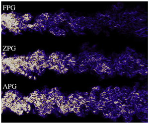
 $5\times 10^{-3}$, which produced a maximum Courant number of 1.15. Figure 2 shows an instantaneous snapshot of the Q-criterion (Jeong & Hussain Reference Jeong and Hussain1995), coloured by the spanwise vorticity for the cases F2, Z and A2, to demonstrate the range of length scales being resolved as well as offering a visual distinction of structures between the three cases. Here,
 $Q=0.5(|\unicode[STIX]{x1D6FA}|^{2}-|S|^{2})$, where
 $|\unicode[STIX]{x1D6FA}|$ and
 $|S|$ are the mean rotation and strain rates respectively.
Instantaneous snapshot of the Q-criterion for cases F2, Z and A2, coloured by the spanwise vorticity.

List of pressure gradient cases simulated. Symbols shown here are used in all line plots. Mean entropy generation rates from the viscous and thermal contributions also shown at  $x_{1}=50$.

3 Results
3.1 Mean statistics
The time-averaged statistics shown in this section were collected over 1800 time units, following a time convergence test, which corresponds with 18 flow-through times. The data presented henceforth are spanwise and time averaged. Given that we solve for the conservative variables ((2.1), (2.2) and (2.3)), the averaging performed is of the Favre-decomposition type, such that any variable  $\unicode[STIX]{x1D719}=\widetilde{\unicode[STIX]{x1D719}}+\unicode[STIX]{x1D719}^{\prime \prime }$, where
 $\widetilde{\unicode[STIX]{x1D719}}=\overline{\unicode[STIX]{x1D70C}\unicode[STIX]{x1D719}}/\overline{\unicode[STIX]{x1D70C}}$ is the Favre average;
 $\overline{\unicode[STIX]{x1D719}}$ corresponds to the Reynolds average such that
 $\unicode[STIX]{x1D719}=\overline{\unicode[STIX]{x1D719}}+\unicode[STIX]{x1D719}^{\prime }$, while
 $\unicode[STIX]{x1D719}^{\prime }$ (Reynolds-decomposed fluctuation) and
 $\unicode[STIX]{x1D719}^{\prime \prime }$ (Favre-decomposed fluctuation) are related by
 $\unicode[STIX]{x1D719}^{\prime \prime }=\unicode[STIX]{x1D719}^{\prime }-\overline{\unicode[STIX]{x1D70C}\unicode[STIX]{x1D719}^{\prime }}/\overline{\unicode[STIX]{x1D70C}}$. Favre decomposition is a popular choice for variable density flows as it provides a strong analogy for variable density effects, arising from the density fluctuation correlations, with constant density flows (Chassaing et al. Reference Chassaing, Antonia, Anselmet, Joly, Sarkar and Moreau2002).
Free-stream variation of (a) mean streamwise velocity, (b) density and (c) pressure at  $x_{2}=20$ units: ● (black), Z; ▪ (red), A1; ♦ (red), A2; ▴ (blue), F1;


Figure 3 shows the streamwise variation of the streamwise velocity, density and pressure in the free stream, at  $x_{2}=20$. The trends confirm the expected changes in the velocity, i.e. acceleration from FPG and deceleration from APG respectively. Due to the pressure gradients acting in a constant area section, the change in the velocity is reciprocated by a change in the density. So, increase in the velocity corresponds to a decrease in density while decrease in the velocity results in density increase. The impact of the pressure gradients are now assessed on the wake by considering a streamwise location within the region of the applied forcing, i.e. at
 $x_{1}=50$. Figure 4 shows the mean streamwise velocity, density and mean cross-stream velocity at
 $x_{1}=50$. The changes in
 $\overline{\unicode[STIX]{x1D70C}}$ and
 $\widetilde{u}_{1}$ are consistent with the changes seen in the free stream. The changes are also consistent with the conservation of mass as the integrated flux (
 $\int \overline{\unicode[STIX]{x1D70C}}\widetilde{u}_{1}\,\text{d}x_{2}$) values are identical across all the cases. The cross-stream velocity (
 $\widetilde{u}_{2}$) shows that the velocity at the boundaries (
 $x_{2}=-20,20$) is zero, which is a direct consequence of the periodic boundary condition as well as the inflow condition. As one moves inward from the boundaries, opposite trends are observed in the adverse and favourable pressure gradients. For APGs, the flow accelerates away from the centreline, peaks a certain distance away and then decelerates until the flow moving outwards comes to a rest at the boundary; while for the favourable gradients, the flow accelerates inward from the boundaries, peaks and then decelerates to zero at the centreline. Following these differences, the wake parameters, namely maximum wake deficit (
 $U_{d}$) and wake half-width (
 $\unicode[STIX]{x1D6FF}$) are plotted in log–log coordinates in figure 5. Also plotted in the figures are lines of slopes
 $-0.5$ for
 $U_{d}$ and 0.5 for
 $\unicode[STIX]{x1D6FF}$. For the ZPG,
 $U_{d}$ and
 $\unicode[STIX]{x1D6FF}$ follow the established scaling laws of
 ${\sim}x_{1}^{-0.5}$ and
 ${\sim}x_{1}^{0.5}$ respectively. In the case of pressure gradients, the development of
 $U_{d}$ is similar to observations in the experimental finding of Liu et al. (Reference Liu, Thomas and Nelson2002), where a pressure gradient was applied in a variable area section. Due to the acceleration of the flow,
 $U_{d}$ reduces in the case of FPGs as the wake profiles tend toward uniformity, while the deceleration caused by APGs affects the centreline more severely than the free stream, causing an increase in the deficit. However, the development of
 $\unicode[STIX]{x1D6FF}$ is different when compared to the experiment. For the pressure gradients, the small deviations from the ZPG case are in contrast to the exponential growth in
 $\unicode[STIX]{x1D6FF}$ for the APG and a constant
 $\unicode[STIX]{x1D6FF}$ for the FPG in the experiment. These differences in the half-width development downstream can be explained by the effect the constant area section imposes on the wake. This can be explained by considering the
 $\widetilde{u}_{2}$ profiles in figure 4 which go to zero at the
 $x_{2}$ boundaries. This imposition restricts the amount of mass flux entering and exiting for the FPG and APG cases, respectively, which would not be the case in the variable area set-up were a similar rectangular control volume considered. In fact, in that situation, there would exist a distribution of
 $\widetilde{u}_{2}$ as a function of
 $x_{1}$ at the
 $x_{2}$ boundaries. Thus, the confinement of the wake in the constant area case alters the spreading of the wake when compared with the conventional variable area case. As opposed to the variable area case, where there is only one macro-length scale, in this study there are two macro-length scales, the width of the domain in addition to the wake half-width. The effect of changing the width of the domain on
 $\unicode[STIX]{x1D6FF}$ will be further elaborated in § 3.4.
(a) Mean streamwise velocity, (b) density and (c) cross-stream velocity at  $x_{1}=50$. For labels, refer to table 1.

(a) Maximum velocity deficit ( $U_{d}$) and (b) wake half-width (
 $\unicode[STIX]{x1D6FF}$) variation with
 $x_{1}$. Solid line represents the slope on the log space plots.

(a) Scaling for  $U_{s}$,
 $U_{d}$ and
 $\unicode[STIX]{x1D6FF}$. The solid line corresponds to a slope of
 $-1$. (b) Self-similarity profile for all cases at
 $x_{1}=50$ units. Dashed line represents (3.1).

Figure 6 shows the proposed scaling between the wake parameters, where  $U_{s}U_{d}/\unicode[STIX]{x1D6FF}\sim x_{1}^{-1}$ was observed empirically. This is different from the scaling proposed by Liu et al. (Reference Liu, Thomas and Nelson2002), where the variation of
 $U_{d}/\unicode[STIX]{x1D6FF}$ was observed to be independent of the pressure gradient. In this study, however, the difference in
 $U_{d}/\unicode[STIX]{x1D6FF}$ at various streamwise locations between the cases could not be ignored, even if the development was very similar. This can clearly be attributed to the way
 $\unicode[STIX]{x1D6FF}$ evolves spatially in the constant area section of this study. The data also reveal that, both in the present study and in the variable area experiments of Liu et al. (Reference Liu, Thomas and Nelson2002), the self-similarity profile of Wygnanski et al. (Reference Wygnanski, Champagne and Marasli1986) is valid:
 $$\begin{eqnarray}\frac{U_{s}-\widetilde{u}_{1}}{U_{d}}=\exp \left(-0.637\left(\frac{x_{2}}{\unicode[STIX]{x1D6FF}}\right)^{2}-0.056\left(\frac{x_{2}}{\unicode[STIX]{x1D6FF}}\right)^{4}\right)\equiv f(x_{2}/\unicode[STIX]{x1D6FF}).\end{eqnarray}$$
Figure 6 shows the self-similar plots of the different cases at  $x_{1}=50$, with all cases collapsing onto the exponential presented in (3.1). The negative values for
 $|x_{2}/\unicode[STIX]{x1D6FF}|\in [2,6]$ units for all cases is due to the velocity excess resulting from the blockage effect produced by the bluff body used.
3.2 Energy budgets
To further our understanding of the trends from the previous section, select budgets of the turbulence kinetic energy ( $\widetilde{k}=0.5\widetilde{u_{i}^{\prime \prime }u_{i}^{\prime \prime }}$) equation are discussed for comparison. The equation used for comparison is the Favre-averaged form, derived by Adumitroaie, Ristorcelli & Taulbee (Reference Adumitroaie, Ristorcelli and Taulbee1999):
 $$\begin{eqnarray}\displaystyle \frac{\unicode[STIX]{x2202}(\overline{\unicode[STIX]{x1D70C}}\widetilde{k})}{\unicode[STIX]{x2202}t}+\underbrace{\frac{\unicode[STIX]{x2202}(\overline{\unicode[STIX]{x1D70C}}\widetilde{k}\widetilde{u}_{j})}{\unicode[STIX]{x2202}x_{j}}}_{{\mathcal{C}}} & = & \displaystyle \underbrace{-\overline{\unicode[STIX]{x1D70C}}\widetilde{u_{i}^{\prime \prime }u_{j}^{\prime \prime }}\frac{\unicode[STIX]{x2202}\widetilde{u}_{i}}{\unicode[STIX]{x2202}x_{j}}}_{{\mathcal{P}}}-\underbrace{\frac{\unicode[STIX]{x2202}(\overline{\unicode[STIX]{x1D70C}}\widetilde{u_{j}^{\prime \prime }k}-\overline{u_{i}^{\prime \prime }\unicode[STIX]{x1D70E}_{ji}\{u^{\prime \prime }\}}+\overline{p^{\prime }u_{j}^{\prime \prime }})}{\unicode[STIX]{x2202}x_{j}}}_{{\mathcal{T}}}\nonumber\\ \displaystyle & & \displaystyle +\,\underbrace{\overline{p^{\prime }\frac{\unicode[STIX]{x2202}u_{i}^{\prime \prime }}{\unicode[STIX]{x2202}x_{i}}}}_{\unicode[STIX]{x1D6F1}}+\underbrace{\overline{u_{j}^{\prime \prime }}\frac{\unicode[STIX]{x2202}\unicode[STIX]{x1D70E}_{ji}\{\widetilde{u}\}}{\unicode[STIX]{x2202}x_{j}}}_{{\mathcal{V}}}-\underbrace{\overline{u_{j}^{\prime \prime }}\frac{\unicode[STIX]{x2202}\overline{p}}{\unicode[STIX]{x2202}x_{j}}}_{{\mathcal{R}}}-\underbrace{\overline{\unicode[STIX]{x1D70E}_{ji}\{u^{\prime \prime }\}\frac{\unicode[STIX]{x2202}u_{i}^{\prime \prime }}{\unicode[STIX]{x2202}x_{j}}}}_{{\mathcal{E}}},\end{eqnarray}$$
where  ${\mathcal{C}}$, convection/advection;
 ${\mathcal{P}}$, production by the mean velocity gradient;
 ${\mathcal{T}}$, turbulent transport;
 $\unicode[STIX]{x1D6F1}$, pressure–dilatation correlation;
 ${\mathcal{V}}$, viscous stress work associated with velocity fluctuations;
 ${\mathcal{R}}$, pressure–work associated with velocity fluctuations; and
 ${\mathcal{E}}$, dissipation due to molecular effects. The term
 $\unicode[STIX]{x1D70E}_{ij}\{\unicode[STIX]{x1D6F7}\}$ refers to the traceless strain rate tensor for the vector
 $\unicode[STIX]{x1D731}$, i.e. replacing
 $u_{i}$ with
 $\unicode[STIX]{x1D6F7}$ in (2.4).
3.2.1 Production
The budget of the production term ( ${\mathcal{P}}$) along the wake centreline (
 $x_{2}=0$) and at
 $x_{1}=50$ is shown in figure 7. While the data presented in this and the following sections are time converged, they has been smoothed out using the Savitzky–Golay filter (Savitzky & Golay Reference Savitzky and Golay1964) to remove fluctuations arising from the higher-order nature of the statistics. The filter preserves the trends, thus allowing ease in visualising the differences between the different cases. The trends suggest that APGs augment the production of
 $\widetilde{k}$ while FPGs reduce it, compared to the ZPG scenario. The wake centreline trend also suggests the same, even though the region shown is upstream of the pressure gradient imposition (
 $x_{1}=25$). For the FPG, there exist regions with negative production at
 $x_{1}=50$, so, to understand these trends, we decompose the production budget into a dilatational production (
 ${\mathcal{P}}_{d}$) component and a shear production (
 ${\mathcal{P}}_{s}$) component as suggested by Liu & Thomas (Reference Liu and Thomas2004),
 $$\begin{eqnarray}\displaystyle & \displaystyle {\mathcal{P}}_{d}=-\overline{\unicode[STIX]{x1D70C}}\widetilde{u_{1}^{\prime \prime }u_{1}^{\prime \prime }}\frac{\unicode[STIX]{x2202}\widetilde{u}_{1}}{\unicode[STIX]{x2202}x_{1}}-\overline{\unicode[STIX]{x1D70C}}\widetilde{u_{2}^{\prime \prime }u_{2}^{\prime \prime }}\frac{\unicode[STIX]{x2202}\widetilde{u}_{2}}{\unicode[STIX]{x2202}x_{2}}, & \displaystyle\end{eqnarray}$$
 $$\begin{eqnarray}\displaystyle & \displaystyle {\mathcal{P}}_{s}=-\overline{\unicode[STIX]{x1D70C}}\widetilde{u_{1}^{\prime \prime }u_{2}^{\prime \prime }}\frac{\unicode[STIX]{x2202}\widetilde{u}_{1}}{\unicode[STIX]{x2202}x_{2}}-\overline{\unicode[STIX]{x1D70C}}\widetilde{u_{2}^{\prime \prime }u_{1}^{\prime \prime }}\frac{\unicode[STIX]{x2202}\widetilde{u}_{2}}{\unicode[STIX]{x2202}x_{1}}, & \displaystyle\end{eqnarray}$$
and this is shown in figure 8. As was observed in the case of Liu & Thomas (Reference Liu and Thomas2004), the dilatational production augments overall production for APGs and vice versa. Given that the pressure gradient magnitudes are higher in this study, the strong FPG’s dilatational component is larger in magnitude than the shear component, leading to overall negative production. This negative production plays a role in transfer of energy from the turbulence to the mean kinetic energy ( $\widetilde{K}=0.5\widetilde{u}_{i}\widetilde{u}_{i}$). Since the normal components of the Reynolds stress in
 ${\mathcal{P}}_{d}$ are positive, the sign of
 ${\mathcal{P}}_{d}$ is driven by
 $\unicode[STIX]{x2202}\widetilde{u}_{1}/\unicode[STIX]{x2202}x_{1}$ and
 $\unicode[STIX]{x2202}\widetilde{u}_{2}/\unicode[STIX]{x2202}x_{2}$. In the case of FPGs,
 $\unicode[STIX]{x2202}\widetilde{u}_{1}/\unicode[STIX]{x2202}x_{1}>0$ since each point undergoes acceleration in the streamwise direction while for APGs
 $\unicode[STIX]{x2202}\widetilde{u}_{1}/\unicode[STIX]{x2202}x_{1}<0$. The value of
 $\unicode[STIX]{x2202}\widetilde{u}_{2}/\unicode[STIX]{x2202}x_{2}$ on the other hand changes sign across
 $x_{2}$. However, at any given spatial position, APG and FPG have the opposite sign (see figure 4). Between the centreline and the location of absolute maximum of
 $\widetilde{u}_{2}$,
 $\unicode[STIX]{x2202}\widetilde{u}_{2}/\unicode[STIX]{x2202}x_{2}>0$ for the APG and
 $\unicode[STIX]{x2202}\widetilde{u}_{2}/\unicode[STIX]{x2202}x_{2}<0$ for the FPG. These values combined explain the difference in the sign of the dilatational component between the different pressure gradients. It is also worth mentioning that the production in the wake centreline is dependent on the dilatational component only and is not affected by the shear production, given the shear stress is zero at the centreline. The trends observed in the production budget show strong similarities to the variable area pressure gradient study of Liu et al. (Reference Liu, Thomas and Nelson2002).
Production budget (a) along wake centreline and (b) at  $x_{1}=50$.

Split of production budget into (a) dilatational component and (b) shear component at  $x_{1}=50$.

3.2.2 Pressure–dilatation correlation and dissipation
The pressure–dilatation correlation ( $\unicode[STIX]{x1D6F1}$) is a budget term that exists only in the compressible formulation of the turbulence kinetic energy budget equation and as such serves to facilitate the transfer of energy between the turbulence kinetic and mean internal energy (
 $\widetilde{e}=\widetilde{T}/\unicode[STIX]{x1D6FE}(\unicode[STIX]{x1D6FE}-1)M_{\infty }^{2}$). When
 $\unicode[STIX]{x1D6F1}>0$, it acts as a source in the turbulence kinetic energy equation, i.e. it helps increase
 $\widetilde{k}$ while
 $\unicode[STIX]{x1D6F1}<0$ increases
 $\widetilde{e}$ at the expense of
 $\widetilde{k}$. At
 $x_{1}=50$, all
 $\unicode[STIX]{x1D6F1}$ values, as shown in figure 9, are negative, causing a reduction in the turbulence kinetic energy. In case of APGs, the magnitude is greater, consequently transferring more energy from the turbulence kinetic to the mean internal energy than the FPGs. However, considering
 $\unicode[STIX]{x1D6F1}$ in isolation is not helpful when dealing with the mechanics of the energy transfer, as will be discussed in a later section.
(a) Pressure–dilatation correlation ( $\unicode[STIX]{x1D6F1}$) and (b) dissipation (
 ${\mathcal{E}}$) at
 $x_{1}=50$.

For the dissipation budget presented in figure 9, the same trend is observed as with other budgets, i.e. APGs demonstrating larger magnitudes than FPGs. Unlike the experiment of Liu (Reference Liu2001), scaling of  ${\mathcal{E}}$ by
 $\unicode[STIX]{x1D6FF}/\widetilde{k}_{max}^{1.5}$ does not show a collapse that would indicate no effect of pressure gradients (not plotted here). Instead, the same trend as with the unscaled dissipation is observed. This could possibly be due to a difference in the development of
 $\unicode[STIX]{x1D6FF}$, which is a direct consequence of the wake evolving in the constant area section.
3.2.3 Pressure work
The pressure work is an important budget term for flows that accelerate or decelerate as it contains the pressure gradient. It appears in two forms, turbulent pressure work ( ${\mathcal{R}}$) and pressure work of the mean (
 $\widetilde{{\mathcal{R}}}$)
 $$\begin{eqnarray}{\mathcal{R}}=\overline{u_{j}^{\prime \prime }}\frac{\unicode[STIX]{x2202}\overline{p}}{\unicode[STIX]{x2202}x_{j}};\quad \widetilde{{\mathcal{R}}}=\widetilde{u}_{j}\frac{\unicode[STIX]{x2202}\overline{p}}{\unicode[STIX]{x2202}x_{j}}.\end{eqnarray}$$
While  ${\mathcal{R}}$ appears in the turbulence kinetic energy equation as a sink and in the mean internal energy equation as a source,
 $\widetilde{{\mathcal{R}}}$ appears in the mean kinetic energy (
 $\widetilde{K}$) as a sink and in the mean internal energy as a source. So, positive values of
 ${\mathcal{R}}$ and
 $\widetilde{{\mathcal{R}}}$ will reduce
 $\widetilde{k}$ and
 $\widetilde{K}$, respectively, and vice versa. Figure 10 shows
 ${\mathcal{R}}$ and
 $\widetilde{{\mathcal{R}}}$ at
 $x_{1}=50$, where we observe all pressure gradients having opposite signs in the two budgets. For
 ${\mathcal{R}}$, the APGs have a negative value while the FPGs have positive values. This indicates that
 ${\mathcal{R}}$, in the case of APGs, contributes to increasing
 $\widetilde{k}$ at the expense of
 $\widetilde{e}$ while FPGs decrease
 $\widetilde{k}$. However, the absolute values of
 ${\mathcal{R}}$ are two orders of magnitude smaller than other budgets of the turbulence kinetic energy, so its impact on
 $\widetilde{k}$ is insignificant. This quantity is not presented in the budgets of Liu et al. (Reference Liu, Thomas and Nelson2002) since the incompressible form of the turbulence kinetic energy is devoid of
 ${\mathcal{R}}$, given that the time mean of the Reynolds fluctuation is zero whereas the time mean of the Favre fluctuation is not. In the case of
 $\widetilde{{\mathcal{R}}}$, budget magnitudes are significantly larger and influence the energy transfer between the mean kinetic and mean internal energies. Clearly, negative values of
 $\widetilde{{\mathcal{R}}}$ would increase the mean kinetic energy, which is expected in the case of accelerating flows (FPGs). A detailed explanation of the energy transfer is presented in the following section.
(a) Pressure work of the fluctuations ( ${\mathcal{R}}$) and (b) of the mean (
 $\widetilde{{\mathcal{R}}}$) at
 $x_{1}=50$.

3.2.4 Energy transfer
Based on the budget trends discussed in the previous sections, the energy transfer sequence is now explored. The interplay of transfer between the different energies is taken from the schematic in Chassaing et al. (Reference Chassaing, Antonia, Anselmet, Joly, Sarkar and Moreau2002), adapted here in figure 11. The condition on a budget near an arrow head signifies transfer of energy from the source of the arrow to the arrow head. For example, a positive value of mean pressure work ( $\widetilde{{\mathcal{R}}}>0$) transfers energy from the mean kinetic to the mean internal energy. This would result in a decrease in the mean kinetic energy while causing an increase in the mean internal energy. The dissipation budget has not been added in the schematic as the transfer is one way, from
 $\widetilde{k}$ to
 $\widetilde{e}$, while the purpose of this section is to analyse the two-way transfer and it’s impact on the energies.
Schematic of energy transfer based on select budgets. Adapted from Chassaing et al. (Reference Chassaing, Antonia, Anselmet, Joly, Sarkar and Moreau2002).

Figure 12 shows the profiles at  $x_{1}=50$ for the turbulent kinetic energy (
 $\widetilde{k}=0.5\widetilde{u_{i}^{\prime \prime }u_{i}^{\prime \prime }}$), the mean internal energy (
 $\widetilde{e}=\widetilde{T}/\unicode[STIX]{x1D6FE}(\unicode[STIX]{x1D6FE}-1)M_{\infty }^{2}$) and the mean kinetic energy (
 $\widetilde{K}=0.5\widetilde{u_{i}}\widetilde{u_{i}}$). Since
 ${\mathcal{R}}$ is smaller than all other budgets shown, its contribution in assessing the energy transfer will be ignored. Looking at the mean internal energy, an increase in the energy is possible when
 $\widetilde{{\mathcal{R}}}>0$ and
 $\unicode[STIX]{x1D6F1}<0$. For APGs, both conditions hold true while for FPGs,
 $\widetilde{{\mathcal{R}}}<0$ and
 $\unicode[STIX]{x1D6F1}<0$. Since
 $\unicode[STIX]{x1D6F1}$ is two orders of magnitude smaller than
 $\widetilde{{\mathcal{R}}}$, the transfer is dominated by the mean pressure work. As a result, APGs have a higher proportion of internal energy. In the case of the mean kinetic energy, the FPGs augment the energy due to smaller (for case F1) or negative (for case F2) production values and negative
 $\widetilde{{\mathcal{R}}}$, while the opposite is true for the APGs. Thus, mean kinetic energy is larger in the case of favourable gradient conditions. Finally, in the turbulence kinetic energy, the net balance of energy transfer is first obtained for each case since
 $\unicode[STIX]{x1D6F1}$ and
 ${\mathcal{P}}$ are comparable in magnitude. If
 $\unicode[STIX]{x1D6F1}+{\mathcal{P}}>0$, an increase in turbulence kinetic energy should be observed. Figure 13 shows that the APGs have larger positive values and consequently help increase the turbulence kinetic energy, while FPGs would cause a reduction in the turbulence kinetic energy.
(a) Turbulence kinetic energy, (b) mean internal energy and (c) mean kinetic energy at  $x_{1}=50$.

Sum of production and pressure–dilatation correlation budgets at  $x_{1}=50$.

3.3 Entropy generation
Turbomachinery design is driven by the aim to minimise loss as it directly affects the aerodynamic efficiency. In Denton (Reference Denton1993), several metrics were introduced to quantify loss, with the case being made for entropy as a preferred candidate, due to its independence of the frame of reference. The total loss could also be obtained by simply summing the entropy changes across the different contributing mechanisms.
Mean entropy generation rates due to viscous and thermal effects at  $x_{1}=50$.

With availability of DNS data, we can take the use of entropy even further, by utilising the entropy generation rate to compute and compare the loss production between the three pressure gradient cases. This is based on the application of the principle of second law analysis, described in Herwig & Schmandt (Reference Herwig and Schmandt2014), by considering the entropy generation rate to assess sources of loss as field information, volume integration of which would provide one final value of the total entropy produced. Another reason for relying on entropy is the fact that entropy and its generation is non-negative, providing an absolute reference of zero, which would correspond to an idealistic process, i.e. zero entropy production. Following the derivation of the entropy generation rate in Bejan (Reference Bejan1982), the instantaneous entropy generation rate for a differential element can be written as
 $$\begin{eqnarray}{\dot{S}}_{gen}=\underbrace{\frac{\unicode[STIX]{x1D705}}{T^{2}}\left(\frac{\unicode[STIX]{x2202}T}{\unicode[STIX]{x2202}x_{i}}\right)^{2}}_{{\dot{S}}_{th}}+\underbrace{\frac{1}{T}\unicode[STIX]{x1D70E}_{ij}\frac{\unicode[STIX]{x2202}u_{i}}{\unicode[STIX]{x2202}x_{j}}}_{{\dot{S}}_{vi}},\end{eqnarray}$$
where the first term ( ${\dot{S}}_{th}$) corresponds to entropy generation due to thermal effects, with
 $\unicode[STIX]{x1D705}$ being the thermal conductivity, while the second term (
 ${\dot{S}}_{vi}$) corresponds to entropy generation due to viscous effects. Here,
 $\unicode[STIX]{x1D70E}_{ij}$ represents the traceless molecular stress tensor, given in (2.4). It is worth mentioning that
 ${\dot{S}}_{gen}$ is independent of the forcing term and for proof of the derivation, the reader is referred to the course notes of Cantwell (Reference Cantwell2018). Manipulation of the second term would reveal that
 ${\dot{S}}_{vi}$ is non-negative, giving a non-negative
 ${\dot{S}}_{gen}$. The total entropy generated can then be obtained by integrating over the volume of interest. While these quantities are all instantaneous, mean entropy generation rate can also be calculated, as performed by Lin, Yuan & Su (Reference Lin, Yuan and Su2017), where the mean values of generation rates are given by
 $$\begin{eqnarray}{\dot{S}}_{\widetilde{vi}}=\frac{1}{\widetilde{T}}\unicode[STIX]{x1D70E}_{ij}\{\widetilde{u}\}\frac{\unicode[STIX]{x2202}\widetilde{u}_{i}}{\unicode[STIX]{x2202}x_{j}},\quad {\dot{S}}_{\widetilde{th}}=\frac{\overline{\unicode[STIX]{x1D705}}}{\widetilde{T}^{2}}\left(\frac{\unicode[STIX]{x2202}\widetilde{T}}{\unicode[STIX]{x2202}x_{i}}\right)^{2}.\end{eqnarray}$$
Figure 14 shows the mean viscous and thermal generation rates at  $x_{1}=50$, non-dimensionalised by reference values. Clearly, the viscous effects are dominant over the thermal effects, by two orders of magnitude. This is not entirely surprising, given that temperature variations are small in the cases simulated. Interestingly, however, the generation rates are negligible in the centreline, with the bulk of the generation concentrated in the region of mean maximum shear stress for the viscous component and the shear layer between the wake and free stream for the thermal component. Finally, the figure also yields information regarding the amount of entropy generation. Visually, the adverse gradients seem to produce higher values than the zero and favourable gradients. This can also be quantified by computing the mass-averaged value of the generation rates (see Cumpsty & Horlock (Reference Cumpsty and Horlock2006)), presented in table 1. The values suggest that accelerating the wake produces lower entropy than decelerating the wake, causing a reduced loss in favourable gradients when compared to adverse gradients. This observation is also in agreement with Denton (Reference Denton1993), where the focus was on the mixing loss metric for qualification. The trends observed above were consistent when looking at the instantaneous generation rates as well. However, comparing the instantaneous with the mean generation rate reveals that the unsteady effects significantly dominate the generation rate, as evidenced from figure 15. We only show one case result for brevity because the differences were similar across the other cases.
Instantaneous and mean entropy generation rates due to viscous and thermal effects, for the A1 case. The bounding box in the images above span  $x_{1}\in [25.0,70.0]$ and
 $x_{2}\in [-10.0,10.0]$. For the instantaneous cases, the data are extracted for one spanwise plane, at
 $x_{3}=0$, while the mean cases are spanwise averaged.

Instantaneous entropy generation rate due to viscous effect in the pressure gradient region for F1, Z and A1 cases. Entropy values for all cases are scaled between 0 and  $2\times 10^{-4}$. The bounding box in the images above span
 $x_{1}\in [25.0,70.0]$ and
 $x_{2}\in [-10.0,10.0]$ for each case. The data presented are extracted for one spanwise location, at
 $x_{3}=0$.

Finally, figure 16 shows an instantaneous snapshot of the viscous entropy generation rate for the F1, Z and A1 cases, zoomed into the pressure gradient region i.e.  $x_{1}\in [25.0,70.0]$. The contour values in all three cases were set between 0 and
 $2\times 10^{-4}$ and offer a direct visual comparison of the amount of entropy generated in each case. The presence of a favourable gradient severely diminishes the amount of entropy existing as well as restricting the extent of generation in the cross-stream direction, whereas for the adverse gradient, the widening of the region of entropy generation is clearly visible along with higher levels of entropy generation. Thus, based on the presented data, it can be stated that a increase in the mean kinetic energy results in reduction of entropy while a loss would increase the entropy produced.
3.4 Effect of domain height
As mentioned in § 3.1, there are two macro-length scales in this flow problem, the height of the domain ( $H$) and the wake half-width (
 $\unicode[STIX]{x1D6FF}$). In this section, we analyse the impact of the domain height on the spatial wake development. To reduce the computational expenses, calculations were performed only for the extreme APG (case A2), as it produces the fastest rate of wake spreading amongst all the cases considered thus far. Additionally, all calculations shown in this section were performed using large eddy simulations (LES), utilising the wall-adapted local eddy viscosity model of Nicoud & Ducros (Reference Nicoud and Ducros1999). Using the DNS grid as a benchmark, the optimal LES grid was obtained by coarsening the grid from the DNS resolution and comparing the mean statistics with the DNS results until the differences could not be ignored. The resulting grid for the LES contains
 $672\times 290$ points in plane with 64 Fourier modes (130 physical points) in the span. Figure 17 shows a comparison of the mean streamwise velocity, density and cross-stream velocity between the LES and DNS as a check on the accuracy of the LES.
Comparison between LES ( $672\times 290\times 130$ points) and DNS (
 $1056\times 396\times 130$ points) for case A2, to assess the accuracy of the LES solution. (a) Mean streamwise, (b) density and (c) cross-stream profiles shown for
 $x_{1}=50$.

List of domain heights simulated, where spatial extent is given in terms of  $L\times H\times W$. A2L represents APG case A2, simulated as LES. Symbols shown here are used in all line plots for § 3.4.

For this section, three additional domain heights were simulated, with extents of  $H=80,20$ and
 $10$ units each in the
 $x_{2}$ direction, apart from the original
 $H=40$ units case. The grid resolutions for these cases and corresponding symbols are presented in table 2. For all cases, the grid point distribution in the
 $x_{1},x_{2}$ directions is unchanged from the A2L2 case. In the case of domain heights smaller than 40, i.e. A2L3 and A2L4, the grid points in
 $x_{2}$ beyond the domain extent were removed while for A2L1, additional points were added in the
 $x_{2}$ direction using the same growth rate as for the A2L2 case. In terms of turbomachinery flows, the effect of the different domain heights studied here is analogous to the pitchwise spacing between consecutive blades in the linear cascade. Larger domains result in blades being spaced further apart, which implies less blades for a given row while smaller domains means more blades for the given row. The optimal spacing is chosen based on a number of parameters, primarily to produce the desired power output. In this study, however, the purpose of varying the domain extent is to obtain a more fundamental understanding on the wake spreading and its relation to the domain extent. Figure 18 shows the streamwise variation of the maximum velocity deficit and the wake half-width for all the additional cases. The largest deviation is observed for case A2L4, compared with the other domain extents. This deviation can be attributed to the cross-stream domain extent being narrow enough to interfere with the wake spreading, resulting in wake–wake interaction, which is demonstrated in figure 19, through the instantaneous Q-criterion snapshot for the A2L4 case. The wakes in the figure above and below the middle wake represent the adjacent wakes on account of the periodicity in the cross-stream direction. The deviation in figure 18 occurs when
 $\unicode[STIX]{x1D6FF}\sim 1.5$, which corresponds to 30 % of half of the cross-stream domain height (
 $H/2=5$ units). Interestingly, the deviation in
 $\unicode[STIX]{x1D6FF}$ is also observed for case A2L3, when
 $\unicode[STIX]{x1D6FF}\sim 3.0$, which corresponds to
 $\unicode[STIX]{x1D6FF}$ being
 $30\,\%$ of half of the domain extent (
 $H/2=10$ units). The adjacent wakes seem to influence the subsequent spreading once the wake becomes sufficiently wide. It could be suggested then, that the spreading for case A2L2 could deviate from A2L1 when
 $\unicode[STIX]{x1D6FF}\sim 6$, if the domain were long enough in the streamwise direction. This is of course speculation and a confirmation is possible only when a simulation of a longer domain in the streamwise direction is conducted. Nevertheless, the main takeaway is that the wake spreading is influenced by both the pressure gradient and the domain height. The pressure gradient dictates the spreading when the domain height is large enough while the domain height controls the spreading when it is small enough. The rapid decline in
 $U_{d}$ and
 $\unicode[STIX]{x1D6FF}$ for case A2L4 due to the narrow domain extent presents an important observation, in that, placing APG wakes closer to one another leads to the APG wake behaving more like a wide domain FPG wake.
Values of (a)  $U_{d}$ and (b)
 $\unicode[STIX]{x1D6FF}$, for domain extent cases and symbols described in table 2.

Instantaneous Q-criterion, coloured by spanwise vorticity for A2L4 case. Top and bottom wakes are transforms of the middle wake to demonstrate the periodic effect with domain bounds for each wake being  $x_{1}\in [-5,75]$,
 $x_{2}\in [-5,5]$ and
 $x_{3}\in [0,8]$.

Furthermore, the closeness of the adjacent wakes causes mixing of the wakes, and this will produce a lower entropy loss than the original wide domain APG (case A2L2). Support for this observation can be found in Michelassi et al. (Reference Michelassi, Chen, Pichler and Sandberg2015), where the authors subjected a low pressure turbine to incoming wakes with different pitches. When the incoming wakes were close enough to interact with one another, the mixing of the wakes produced loss values similar to the case of no incoming wakes with background turbulence. This was due to the wakes mixing out before reaching the leading edge of the low pressure turbine, while the other cases produced distinct wakes, resulting in higher loss. Drawing a parallel with our study, closely spacing the wakes can reduce the impact the pressure gradient has, seen through the changes in  $U_{d}$ and
 $\unicode[STIX]{x1D6FF}$, which happen due to the mixing out from wake–wake interaction. Mixing out in wakes refers to the reduction in the non-uniformity or a wake moving towards ‘flatness’. This point is demonstrated through figure 20, which shows the mean streamwise velocity for all the cases at
 $x_{1}=50$, normalised by the domain height. The move towards ‘flatness’ in the wake profile is clearly visible as the domain height shrinks. Finally, figure 20 also shows the streamwise variation of
 $U_{s}U_{d}/\unicode[STIX]{x1D6FF}$, where a reasonable collapse is observed for the different domain extents, meaning the empirical scaling law proposed in § 3.1 still holds.
(a) Mean streamwise velocity at  $x_{1}=50$, scaled by the corresponding domain height and (b) streamwise variation of
 $U_{d}U_{s}/\unicode[STIX]{x1D6FF}$, for domain extent cases and symbols described in table 2.

4 Summary and conclusions
In this study, the impact of constant area pressure gradients on spatial wake development was examined through the use of multiple high-fidelity compressible DNSs. Unlike the traditional method of applying pressure gradients on wakes by changing the cross-sectional area, the commonly occurring wakes in the stator–rotor gap of turbomachines develop under pressure gradients in constant cross-sectional areas. As such, for the first time, we study a canonical set-up of a wake from a bluff body, subjected to a constant area region of pressure gradient. With the Reynolds number and range of gradients considered matching turbine wake conditions, we reported on key time-averaged quantities, such as the streamwise and cross-stream velocities, density and wake parameters. Compared with the conventional application, where the pressure gradients act in a variable area section, the mean statistics reveal non-trivial differences. The change in the streamwise velocity causes a change in the density of the fluid while the constant area condition restricts the variation of the cross-stream velocity. This has an impact on the amount of wake spreading, with the variation in the wake half-width being not significantly different from the zero pressure gradient case.
However, the different pressure gradient cases show a reasonable collapse onto the self-similarity profile proposed by Wygnanski et al. (Reference Wygnanski, Champagne and Marasli1986), and are in agreement with the variable area pressure gradient. The difference in the growth of  $\unicode[STIX]{x1D6FF}$ also reveals a different scaling law, where
 $U_{s}U_{d}/\unicode[STIX]{x1D6FF}$ was observed to scale with
 $x_{1}^{-1}$ compared with the variable area gradient case where
 $U_{d}/\unicode[STIX]{x1D6FF}$ was observed to be independent of the pressure gradient. Following this, a detailed investigation into the energy budgets was conducted, which also revealed key differences. The turbulence production term showed the importance of the dilatational component’s role in the total production. For FPGs, the dilatational component was negative and larger in magnitude than the positive shear component. This resulted in an overall negative production in the pressure gradient region. In the case of dissipation, the pressure gradients demonstrated that they had an impact on its value, even after scaling, which is different than the observations of the variable area gradients. Additional budgets were also presented, which appear only in the compressible version of the turbulence kinetic energy equation. The pressure–dilatation term, which relates the pressure fluctuations with the fluctuation dilatation, was found to be important in the energy transfer between the mean internal energy and the turbulence kinetic energy. The pressure–work term for the fluctuations and mean velocities revealed that the fluctuation contribution was two orders of magnitude smaller than other budgets considered while the mean contribution dominated all other budgets. The latter budget term was found to be important in facilitating the transfer between the mean internal and mean kinetic energies. The energy transfer sequence based on the extracted budgets showed that FPGs added energy to the mean kinetic energy at the expense of the turbulence kinetic and mean internal energy while the adverse gradient extracted energy from the mean kinetic energy to facilitate the turbulence kinetic and mean internal energies.
Subsequently, the entropy generation rates were computed for all the pressure gradient cases, instantaneously and in the mean. The instantaneous entropy generation rates dominated the mean rate by two orders of magnitude and the viscous effects were found to be more important than the thermal effects, again by two orders of magnitude. The FPGs inhibited the production of entropy along with the size of the region, while the APGs did the exact opposite. Thus, the reduction in entropy production achieved by exposing wakes to favourable pressure gradients could serve as a way to help reduce the loss produced.
Finally, the effect of different domain heights in the cross-stream direction ( $x_{2}$) was investigated for the extreme APG case using large eddy simulations. The spreading of the wake was found to depend on the value of the wake half-width
 $\unicode[STIX]{x1D6FF}$ relative to the domain height. It was observed that a deviation in the
 $\unicode[STIX]{x1D6FF}$ growth occurred when it was
 $30\,\%$ of half of the domain height in
 $x_{2}$ and the deviation was explained due to the interaction with adjacent wakes. As a result, both the pressure gradient and the lateral domain extent were found to influence the wake spreading. When wake–wake interaction is negligible, the pressure gradient dictates the wake spreading while the wake–wake interaction affects the wake spreading for narrower domains. This interaction leads to accelerated mixing of the wakes, through slower wake spreading and rapid decline in
 $U_{d}$. Consequently, a reduction in the entropy generation is possible, leading to a scenario where an adverse pressure gradient reduces the loss when wakes are close enough to interact with one another.
Acknowledgements
This work was supported by resources provided by the Pawsey Supercomputing Centre with funding from the Australian Government and the Government of Western Australia. This work is also financially supported by the University of Melbourne PhD Writeup Grant.
Declaration of interests
The authors report no conflict of interest.
Pressure gradient obtained for all cases in table 1 at  $x_{2}=20$. The forcing term variation is also present as a dashed line for each pressure gradient case.

Appendix A. Relating the forcing term to the pressure gradient
To understand the role the forcing term plays in mimicking the pressure gradient, we first extract the pressure gradient in the free stream for all the pressure gradient cases described in table 1. The streamwise variation of the pressure gradient is plotted in figure 21, along with the streamwise variation of the forcing term. The figure shows that the pressure gradient obtained is higher in magnitude than the forcing term for all cases. The pressure gradients in figure 21 are a response to the existence of the forcing term within the momentum equation, in (2.2). Given a pressure field  $\overline{p}^{\ast }$ that needs to be modelled through a forcing term, a comparison of the streamwise momentum equation with and without the forcing term can be made. By combining all the terms of the streamwise momentum equation into the left-hand side of the equality, save for the pressure gradient and forcing term,
 $NS(\widetilde{u}_{1})$, the momentum equations with and without the forcing term are given by
 $$\begin{eqnarray}\displaystyle & \displaystyle NS(\widetilde{u}_{1})=-\frac{\unicode[STIX]{x2202}\overline{p}}{\unicode[STIX]{x2202}x_{1}}+F, & \displaystyle\end{eqnarray}$$
 $$\begin{eqnarray}\displaystyle & \displaystyle NS(\widetilde{u}_{1})=-\frac{\unicode[STIX]{x2202}\overline{p}^{\ast }}{\unicode[STIX]{x2202}x_{1}}. & \displaystyle\end{eqnarray}$$
While (A 2) represents the momentum equation with the actual pressure gradient, (A 1) represents the momentum equation with a forcing term as evaluated by the simulation, to mimic (A 2). Comparing the two, the actual pressure gradient being modelled can be given by
 $$\begin{eqnarray}\frac{\unicode[STIX]{x2202}\overline{p}^{\ast }}{\unicode[STIX]{x2202}x_{1}}=\frac{\unicode[STIX]{x2202}\overline{p}}{\unicode[STIX]{x2202}x_{1}}-F.\end{eqnarray}$$
Based on (A 3), it was observed that, with the different values of the forcing terms, the actual gradient ( $\unicode[STIX]{x2202}\overline{p}^{\ast }/\unicode[STIX]{x2202}x_{1}$) was approximately an order of magnitude smaller that the simulated pressure gradient (
 $\unicode[STIX]{x2202}\overline{p}/\unicode[STIX]{x2202}x_{1}$). This information can thus be used to fix the limits of the forcing term needed to conduct the pressure gradient investigation. Since the LPT pressure gradients downstream of the blade trailing edge were shown to be within
 $-0.008$ and 0.008 (figure 1), our investigation would look at forcing terms between
 $-0.08$ and 0.08. To further elaborate on the relation between the forcing term and the pressure gradient, we can perform a time-averaged volume integral of the streamwise momentum equation, within the region of the applied forcing term, i.e.
 $x_{1}\in [25,70]$. The integrated equation with the dominant terms is given by
 $$\begin{eqnarray}\overline{\unicode[STIX]{x1D70C}}\widetilde{u}_{1}^{2}|_{f}-\overline{\unicode[STIX]{x1D70C}}\widetilde{u}_{1}^{2}|_{i}=\overline{p}|_{i}-\overline{p}|_{f}+F_{o}(x_{1}-25),\end{eqnarray}$$
where the subscripts  $i,f$ correspond to initial and final positions in
 $x_{1}$, while the contribution from the molecular and Reynolds stresses were found to be negligible. The implication of (A 4) is that the net change in momentum flux is balanced by both the pressure difference and the forcing term. Thus, the difference between the solid and dashed lines in figure 21 is the net change in momentum flux. Since the mass flux is fixed, the pressure gradient is a part of the solution, i.e. it is not known until after the simulation is performed. However, with our choice of forcing terms, the resulting pressure gradient was within the limits of the LPT pressure gradients and is thus satisfactory for the present study.



