3.1. Spectral proper orthogonal decomposition

Spectral proper orthogonal decomposition is now a widely used tool for the study of turbulent flows. It decomposes the data into an orthogonal basis ranked in terms of an energy norm, and can provide a useful basis for the description of empirical coherent structures, particularly when the leading eigenvalue is substantially larger than its subdominante counterparts.

In the framework of SPOD, given the state vector, $\boldsymbol {q}=[\rho, u_{x},u_{r}, u_{\theta }, T]^{{\rm T}}$, subject to a Reynolds decomposition,

(3.1)\begin{equation} \boldsymbol{q}(x,r,\theta,t) = \bar{\boldsymbol{q}}(x,r,\theta) + \boldsymbol{q}'(x,r,\theta,t), \end{equation}

optimal modes for a given azimuthal wavenumber and Strouhal number pair, $\boldsymbol {\varPsi }_{m,\omega }$, are obtained through eigendecomposition of the cross-spectral density (CSD) matrix, $\hat {\boldsymbol {S}}_{m,\omega }$,

(3.2)\begin{equation} \hat{\boldsymbol{S}}_{m,\omega}\boldsymbol{\mathsf{W}}\boldsymbol{\varPsi}_{m,\omega} =\boldsymbol{\varPsi}_{m,\omega}\boldsymbol{\varLambda}_{m,\omega}. \end{equation}

The CSD matrix is computed as $\hat {\boldsymbol {S}}_{m,\omega }=\hat {\boldsymbol {Q}}_{m,\omega }\hat {\boldsymbol {Q}}_{m,\omega }^{H}$, where $\hat {\boldsymbol {Q}}_{m,\omega }=[\hat {\boldsymbol {q}}_{m,\omega }^{(1)}\ \hat {\boldsymbol {q}}_{m,\omega }^{(2)} \cdots \hat {\boldsymbol {q}}_{m,\omega }^{(N_{blk})}]$ is the ensemble of $N_{blk}$ flow realisations at $(m,\omega )$, with $\hat {\boldsymbol {q}}_{m,\omega _{k}}^{(l)}$ denoting the $l$th Fourier realisation of the turbulent fluctuations, $\boldsymbol {q}'$, in time and azimuthal direction at the frequency $\omega$ and wavenumber $m$. The superscript $^{H}$ denotes Hermitian transpose.

The eigenvalues, $[\lambda _{m,\omega }^{(1)}, \lambda _{m,\omega }^{(2)} \cdots \lambda _{m,\omega }^{(nblk)}]$ corresponding to the modal energy are organised in decreasing order in the diagonal matrix $\boldsymbol {\varLambda }_{m,\omega }$. The modes so obtained are orthogonal with respect to a given inner product,

(3.3)\begin{equation} \langle \boldsymbol{q}_{1},\boldsymbol{q}_{2}\rangle =\boldsymbol{q}_{1}^{H} \boldsymbol{\mathsf{W}} \boldsymbol{q}_{2}. \end{equation}

Here we consider a weighting matrix, $\boldsymbol{\mathsf{W}}$, describing Chu's compressible energy norm (Chu Reference Chu1965),

(3.4)\begin{equation} \langle \boldsymbol{q}_{1},\boldsymbol{q}_{2}\rangle_{E}=\iiint\boldsymbol{q}_{1}^{H}\,\mathrm{diag} \left(\frac{\bar{T}}{\gamma \bar{\rho}M_{j}^2},\bar{\rho}, \bar{\rho}, \bar{\rho}, \frac{\bar{\rho}}{\gamma(\gamma-1)\bar{T}M_{j}^2} \right)\boldsymbol{q}_{2} r\,\mathrm{d}\kern0.06em x\,\mathrm{d}r \,\mathrm{d}\theta. \end{equation}

The CSDs are computed using Welch's periodogram method. The data was segmented into blocks of 512 samples with 75 % overlap, resulting in a frequency resolution of $\Delta St=0.0217$. Convergence of the SPOD modes was checked by varying the number and length of the blocks in the Welch algorithm, while keeping a suitable frequency resolution. We found that the parameters we used are sufficient to attain converged modes, including in the $St \to 0$ limit. Using larger blocks of 1024 yielded almost identical SPOD modes, although the uncertainty was larger due to the reduced number of blocks. Furthermore, we have also tried the time-shifting SPOD technique recently introduced by Blanco et al. (Reference Blanco, Martini, Sasaki and Cavalieri2022). The main idea of the technique is to align cross-correlations inside each block according to the convection velocity of the underlying flow structures. This helps improving convergence of SPOD modes by increasing the number of blocks available for a given time series, which can be useful for large datasets that usually have a limited number of snapshots. However, application of this technique to our databases did not yield any noticeable improvement on convergence, which indicates that the chosen block size and the number of blocks was already sufficient.

3.2. Resolvent analysis

Since the works of Hwang & Cossu (Reference Hwang and Cossu2010) and McKeon & Sharma (Reference McKeon and Sharma2010), resolvent analysis has been extensively used to identify optimal forcing and response mechanisms in laminar and turbulent flows and to model coherent structures. The analysis starts with the linearised Navier–Stokes equations in frequency domain, expressed in input–output form (Schmidt et al. Reference Schmidt, Towne, Rigas, Colonius and Brès2018),

(3.5) $$\begin{gather} ({\rm i}\omega\boldsymbol{\mathsf{I}}-\boldsymbol{\mathsf{A}}_m)\hat{\boldsymbol{q}}_{m,\omega} = \boldsymbol{\mathsf{B}}\hat{\boldsymbol{f}}_{m,\omega}, \end{gather}$$

(3.6)$$\begin{gather}\hat{\boldsymbol{y}}_{m,\omega} = \boldsymbol{\mathsf{C}}\hat{\boldsymbol{q}}_{m,\omega}, \end{gather}$$

where $\boldsymbol{\mathsf{A}}_m$ is the linearised Navier–Stokes operator, $\hat {\boldsymbol {q}}_{m,\omega }$ is the Fourier-transformed state vector and $\hat {\boldsymbol {f}}_{m,\omega }$ is a term representing the nonlinear Reynolds stresses, which are treated as an endogenous forcing term. The subscript $_{m,\omega }$, with $m$ the azimuthal wavenumber and $\omega$ the frequency, denotes Fourier transform in the azimuthal and time directions. Here $\hat {\boldsymbol {y}}_{m,\omega }$ defines the desired response, or output, as a function of the state; $\boldsymbol{\mathsf{I}}$ is the identity matrix and $\boldsymbol{\mathsf{B}}$ and $\boldsymbol{\mathsf{C}}$ are matrices that can be used to restrict forcing and observation to specific regions of space and/or to a limited number of forcing and response terms.

Input and output are related through

(3.7)\begin{equation} \hat{\boldsymbol{y}}_{m,\omega} = \boldsymbol{R}_{m,\omega}\,\hat{\boldsymbol{f}}_{m,\omega}, \end{equation}

where $\boldsymbol {R}_{m,\omega }$ is the resolvent operator,

(3.8)\begin{equation} \boldsymbol{R}_{m,\omega} = \boldsymbol{\mathsf{C}}({\rm i}\omega\boldsymbol{\mathsf{I}}-\boldsymbol{\mathsf{A}}_m)^{{-}1}\boldsymbol{\mathsf{B}}. \end{equation}

We then define a weighted resolvent operator, $\tilde {\boldsymbol {R}}_{m,\omega }$, by introducing Chu's compressible energy norm through the matrix $\boldsymbol{\mathsf{W}}$,

(3.9)\begin{equation} \tilde{\boldsymbol{R}}_{m,\omega} = \boldsymbol{\mathsf{W}}^{1/2}\boldsymbol{R}_{m,\omega}\boldsymbol{\mathsf{W}}^{{-}1/2}. \end{equation}

The goal of resolvent analysis is to seek an optimal forcing that maximises the norm of the associated flow response,

(3.10) \begin{equation} \sigma_1^2 = \max_{\|\,\hat{{f}}_{m,\omega}\|=1}\frac{\| \tilde{\boldsymbol{R}}_{m,\omega}\,\hat{\boldsymbol{f}}_{m,\omega} \|^{2}_{\boldsymbol{W}}}{\|\,\hat{\boldsymbol{f}}_{m,\omega} \|^{2}_{\boldsymbol{W}}}. \end{equation}

This can be achieved through singular-value decomposition of the resolvent operator,

(3.11)\begin{equation} \tilde{\boldsymbol{R}}_{m,\omega} = \boldsymbol{\mathsf{U}}\boldsymbol{\varSigma}\boldsymbol{\mathsf{V}}^{H}. \end{equation}

Forcing ($\boldsymbol {u}_{i}$) and response ($\boldsymbol {v}_{i}$) modes are defined as $\boldsymbol {v}_{i} = (\boldsymbol {W}^{-1/2})^{H}\boldsymbol {V}_{i}$ and $\boldsymbol {u}_{i} = (\boldsymbol {W}^{-1/2})^{H}\boldsymbol {U}_{i}$, with $i$ denoting the $i$th column of $\boldsymbol{\mathsf{V}}$ and $\boldsymbol{\mathsf{U}}$. The singular values associated with each forcing-response pair, $\sigma _{i}$, are arranged in descending order in the diagonal matrix $\boldsymbol {\varSigma }$. Optimal forcings and responses for each $m, \omega$ pair are then given by $\boldsymbol {v}_{i}$ and $\boldsymbol {u}_{1}$, and their associated energy gain is the square of the leading singular value, $\sigma _1^2$. As in Schmidt et al. (Reference Schmidt, Towne, Rigas, Colonius and Brès2018), the governing equations are discretised using fourth-order summation by parts finite differences (Mattsson & Nordström Reference Mattsson and Nordström2004), the polar singularity is treated as in Mohseni & Colonius (Reference Mohseni and Colonius2000), and non-reflecting boundary conditions/sponges are employed at the domain boundaries. The dominant resolvent modes are computed using randomised linear algebra methods (Martinsson Reference Martinsson2019) that allow for the efficient computation of dominant singular values/vectors.

As mentioned above, we focus on the characterisation of the flight stream effect on the turbulent field, rather than the acoustic field, as done by many previous studies (Von Glahn et al. Reference Von Glahn, Groesbeck and Goodykoontz1973; Bushel Reference Bushel1975; Cocking & Bryce Reference Cocking and Bryce1975; Packman et al. Reference Packman, Ng and Paterson1975; Plumbee Reference Plumbee1975; Morfey & Tester Reference Morfey and Tester1977; Bryce Reference Bryce1984; Viswanathan & Czech Reference Viswanathan and Czech2011). To that end, we restrict the forcing and observation fields to the hydrodynamic region via the matrices $\boldsymbol{\mathsf{B}}$ and $\boldsymbol{\mathsf{C}}$. This is done by setting the elements of those matrices to one within the jet shear layer, delimited by the region where $\bar {U}_x/\bar {U}_j \geq 0.05$, and gradually reducing them to zero for larger $r$. Here we also enforce a mask on the forcing field inside the jet potential core. The reason for this is that the jet supports trapped acoustic waves that resonate, producing a tonal dynamics in the potential core (Schmidt et al. Reference Schmidt, Towne, Colonius, Cavalieri, Jordan and Brès2017; Towne et al. Reference Towne, Cavalieri, Jordan, Colonius, Schmidt, Jaunet and Brès2017). The resonant mechanism at $M_j=0.9$ is such that the jet is marginally globally stable at certain frequencies, and the resolvent analysis thus identifies this resonance mechanism as a leading candidate for optimal growth. This mechanism is not dominant in the SPOD analysis, as we will briefly show, and therefore, we choose to mask it, so as to focus on the dominant turbulent structures. In Appendix A we briefly discuss their presence in the forcing and response modes. Regarding the fact that the trapped waves are more pronounced in the resolvent modes, Schmidt et al. (Reference Schmidt, Towne, Rigas, Colonius and Brès2018) attributes this to two factors: the first is the choice of an effective Reynolds number, which, in our case, corresponds to the choice of the eddy viscosity. In mean-flow-based resolvent models, different mechanisms respond differently to changes in Reynolds number/eddy viscosity, and the choice of these parameters might highlight one mechanism to the detriment of the other (for instance, accentuating trapped waves to the detriment of KH waves). Secondly, the resonance provides an optimal forcing mechanism in the resolvent model; but in the real flow the resonance mechanism might not be forced so efficiently, which would attenuate these waves. Analysis of the effect of nonlinear forcing on trapped waves is outside the scope of this work. We emphasise that these issues are minor in the context of the present work and, as we show in Appendix A, the suppression of these waves does not affect the analysis of the other linear instability mechanisms.

Figure 1 shows the resulting mean-flow masks applied to the forcing and response fields. The goal of the resolvent analysis is therefore to seek an optimal forcing that maximises the compressible energy norm of the associated flow response in the highlighted region.

Figure 1.

Example of mean-flow masks applied to (a) the forcing and (b) the response for the static case, $M_f=0$.

3.2.1. Eddy-viscosity model

The effects of eddy viscosity on the predictive capabilities of linear analysis have been explored in a number of recent studies (Crouch et al. Reference Crouch, Garbaruk and Magidov2007; Hwang & Cossu Reference Hwang and Cossu2010; Oberleithner et al. Reference Oberleithner, Paschereit and Wygnanski2014; Rukes et al. Reference Rukes, Paschereit and Oberleithner2016; Tammisola & Juniper Reference Tammisola and Juniper2016; Schmidt et al. Reference Schmidt, Towne, Rigas, Colonius and Brès2018; Morra et al. Reference Morra, Semeraro, Henningson and Cossu2019; Kuhn et al. Reference Kuhn, Soria and Oberleithner2021; Pickering et al. Reference Pickering, Rigas, Schmidt, Sipp and Colonius2021). The study of Pickering et al. (Reference Pickering, Rigas, Schmidt, Sipp and Colonius2021) showed substantial improvements in the agreement between resolvent response modes and coherent structures educed from flow data through SPOD.

Here we adopt the mean-flow-consistent eddy-viscosity model of Pickering et al. (Reference Pickering, Rigas, Schmidt, Sipp and Colonius2021), which is useful in cases where experimental and numerical databases do not provide an eddy-viscosity field directly, as is the case with the LES database used here. The molecular viscosity, $\mu$, is replaced by the sum $\mu + \mu _T$ in the linearised equations, and a suitable spatial structure for the eddy viscosity, $\mu _T$, is determined, as described below. The resolvent operator can then be rewritten as

(3.12) \begin{equation} \boldsymbol{\mathsf{R}}_{m,\omega} = \boldsymbol{\mathsf{C}}({\rm i}\omega\boldsymbol{\mathsf{I}}-\boldsymbol{\mathsf{A}}_{m} - \boldsymbol{\mathsf{A}}_{m,T}(\mu_T) )^{{-}1}\boldsymbol{\mathsf{B}}, \end{equation}

where $\boldsymbol{\mathsf{A}}_{m,T}$ only possess terms including $\mu _T$. The reader is referred to Pickering et al. (Reference Pickering, Rigas, Schmidt, Sipp and Colonius2021) for the equations for the modified operator. The eddy-viscosity field, $\mu _T(x,r)$, is found by minimising the error by which the mean flow satisfies the zero-frequency, zero-azimuthal wavenumber linearised Navier–Stokes equations, modified with the addition of an eddy-viscosity field. The forcing term, which represents frequency-dependent Reynolds stresses, is approximated through an eddy-viscosity model, and subsequently lumped on the linear operator on the left-hand side. For $\omega =0$ and $m=0$, $\hat {\boldsymbol {q}}_{m,\omega }$ becomes the mean flow itself, $\bar {\boldsymbol {q}}$, which leads to the equation

(3.13) \begin{equation} (\boldsymbol{\mathsf{A}}+\boldsymbol{\mathsf{A}}_{\boldsymbol{\mathsf{T}}})\bar{\boldsymbol{q}}=\bar{f}, \end{equation}

where $\bar {f}$ is a residual term. Note that, if the eddy-viscosity approximation were exact, the left-hand side of (3.13) would be identically zero; but since the model is not exact, there is a residual. We then find the eddy-viscosity field through an optimisation procedure that minimises the following cost function:

(3.14)\begin{equation} \mathcal{J} ={-}\bar{f}\boldsymbol{\mathsf{W}}\bar{f}. \end{equation}

Details about the optimisation algorithm can be found in Pickering et al. (Reference Pickering, Rigas, Schmidt, Sipp and Colonius2021). The optimisation provided order-of-magnitude reductions in the residual. Figure 2 shows the mean-flow-consistent eddy-viscosity fields for the $M_f=0$ and $M_f=0.15$ jets. Their shapes are similar to those obtained previously at lower Mach number (Pickering et al. Reference Pickering, Rigas, Schmidt, Sipp and Colonius2021). Some streamwise waviness can be seen in the fields obtained for both cases. Optimisation of the entire eddy-viscosity field at once leads to a stiff problem prone to numerical errors. To alleviate this, the domain is broken into overlapping subsections, and a block-by-block optimisation is performed. This generates the observed streamwise waviness between adjacent blocks. These differences are numerical artifacts and while they could be carefully tuned and smoothed away, these improvements would only create marginal improvements to the resolvent analysis.

Figure 2.

Mean-flow-consistent eddy-viscosity fields computed at zero frequency and azimuthal wavenumber for (a) the static case, $M_f=0$, and (b) the flight stream case, $M_f=0.15$.

The amplitude of the eddy-viscosity model was scaled by a constant, $\widetilde {\mu _T} = c\mu _T$. This constant is used as a frequency-independent tuning parameter that allows us to improve the alignment between resolvent and SPOD modes (Pickering et al. Reference Pickering, Rigas, Schmidt, Sipp and Colonius2021). Physically, $c$ is necessary as the eddy-viscosity field found through the mean-flow optimisation considers both large- and fine-scale fluctuations. Thus, we consider small values, 0.1–0.2, to represent only the fine-scale eddy-viscosity contribution and effect in modelling the large-scale structures. Here we found $c=0.15$ to provide the best alignment with respect to leading SPOD modes at different frequencies and azimuthal wavenumbers. The physical consistency of this value was verified through a comparison with the Boussinesq approximation, as done by Kuhn et al. (Reference Kuhn, Soria and Oberleithner2021). Using a nonlinear least square algorithm, we have computed the constant values that give the best fit of $\mu _{T}(x,r)$ to the Boussinesq eddy-viscosity field, given by

(3.15)\begin{equation} \mu_{T{_B}} ={-}\frac{\overline{u_x'u_r'}}{\mathrm{d}\bar{U}/\mathrm{d}r}. \end{equation}

This best fit was obtained for values of $c=0.16$ and $c=0.12$ in the static and flight stream cases, respectively, which are quite close to the constant value used in this study. Furthermore, the shapes of the eddy-viscosity fields of the two models were found to be in fair qualitative agreement, which further supports the consistency of the eddy-viscosity model adopted here. We emphasise, though, that the model displays limited sensitivity to the scaling constant, and similar model results can be obtained with other choices of $c$ (albeit with a reduced alignment with respect to SPOD). In Appendix B we explore resolvent analyses conducted with $c=0.10$ and $c=0.20$. Overall, the trends are similar to the results presented in §§ 4 and 5 for $c=0.15$, indicating that the main results of this study (and its main conclusions) are not restricted to a specific choice of scaling parameter. Furthermore, this constant was also found to be remarkably robust between different cases of the same jet. For instance, Heidt et al. (Reference Heidt, Colonius, Nekkanti, Schmdit, Maia and Jordan2021) showed that a constant tuned for a natural jet at $Ma=0.4$ could be used, with the same level of accuracy, when the jets are forced at different frequencies and amplitudes.

5.1. KH mechanism

The modal KH mechanism is dominant over a broad frequency range, $St \gtrsim 0.2$ (Schmidt et al. Reference Schmidt, Towne, Rigas, Colonius and Brès2018; Lesshafft et al. Reference Lesshafft, Semeraro, Jaunet, Cavalieri and Jordan2019; Pickering et al. Reference Pickering, Rigas, Nogueira, Cavalieri, Schmidt and Colonius2020), and can be observed up to $St=4$ and $m=4$ near the nozzle region (Sasaki et al. Reference Sasaki, Cavalieri, Jordan, Schmidt, Colonius and Brès2017). Here we present results for the axisymmetric azimuthal mode at $St=0.6$ as a representative case where KH wavepackets are clear in the jet response. Similar trends were found for other azimuthal wavenumbers and Strouhal numbers within the KH-dominated region of the spectrum, indicated in figure 6. Figures 8 and 9 show leading forcing, $\boldsymbol {v}_1$, and response, $\boldsymbol {u}_1$, modes for the static and flight cases, respectively. The leading SPOD mode of streamwise velocity is also shown for comparison, and is in striking agreement with the leading response mode in both cases, consistent with the alignment metric shown in figure 6. The forcing modes exhibits Orr-like structures localised in the vicinity of the nozzle lip, and are in agreement with observations made at lower-Mach-number jets (Garnaud et al. Reference Garnaud, Lesshafft, Schmid and Huerre2013; Schmidt et al. Reference Schmidt, Towne, Rigas, Colonius and Brès2018; Lesshafft et al. Reference Lesshafft, Semeraro, Jaunet, Cavalieri and Jordan2019). Similar structures have also been observed within the nozzle boundary layer (Kaplan et al. Reference Kaplan, Jordan, Cavalieri and Brès2021). Figures 8(b) and 9(b) show the streamwise evolution of the response and forcing amplitudes for each velocity component. The curves correspond to the local compressible inner products, $|\boldsymbol {u}_1^{H}\boldsymbol{\mathsf{W}}\boldsymbol {u}_1|$ and $|\boldsymbol {v}_1^{H}\boldsymbol{\mathsf{W}}\boldsymbol {v}_1|$ for the resolvent, and $|\varPsi _1^{H}\boldsymbol{\mathsf{W}}\varPsi _1|$ for the SPOD modes, at each streamwise position. Note that the $u_\theta$ component is null for the axisymmetric mode. The amplitudes of those curves is arbitrary, as SPOD and resolvent modes are not scaled by modal energy and gains, respectively (this also applies to figures 10–13). The growth rates of the resolvent response modes are found to be significantly larger than those of the SPOD modes (the modes are scaled so as to have the same amplitudes at $x/x_c=0$). However, they attain saturation at roughly the same streamwise position. Furthermore, as mentioned above, the shapes are in very good agreement, indicating that the main mechanism is well captured by the model. The forcing amplitudes display a noisy behaviour in the initial jet region, as opposed to the smooth decay observed at a lower Mach number (Pickering et al. Reference Pickering, Rigas, Nogueira, Cavalieri, Schmidt and Colonius2020). This behaviour is due to the signature of trapped waves. Despite the mask in the potential core being able to significantly attenuate these waves (see, for instance, the results of figure 17 without the core mask), it does not eliminate them altogether. A more efficient way to suppress them completely would be to also restrict the response at the jet core; but this would also impact the growth of KH waves in that zone and, therefore, it has not been done here. The structure of KH wavepackets in static and flight conditions are found to be quite similar (which can also be inferred from the alignment maps of figure 7). With the potential core scaling, the regions of exponential, growth, stabilisation and decay are found to be quite similar. Note that the SPOD modes do not display clear signs of trapped waves, although no mask has been applied in the SPOD computation. In Appendix A we show that the mechanism of the trapped waves is present in the SPOD as well, but their energy is much smaller than that of KH wavepackets. They can be clearly seen in the response modes if the amplitude of the KH waves is artificially reduced, as shown in figure 17. Moreover, they appear more clearly in the second SPOD mode, which is not considered in this section.

Figure 8.

(a) Leading forcing and response modes of the axisymmetric wavenumber $m=0$ and Strouhal number $St=0.6$ for the static case, $M_f=0$. Leading SPOD mode is also shown for comparison. The modes are shown with contours corresponding to $\pm 0.7\|u_{x,r}\|$. (b) Component-wise amplitudes as a function of streamwise coordinate, computed through the compressible energy norm.

Figure 9.

Leading forcing and response modes of the axisymmetric wavenumber $m=0$ and Strouhal number $St=0.6$ for the flight case, $M_f=0.15$. Legend is as in figure 8.

Figure 10.

Leading forcing and response modes of the axisymmetric wavenumber $m=0$ and Strouhal number $St=0.2$ for the static case, $M_f=0$. Legend is as in figure 8.

Figure 11.

(a) Leading forcing and response modes of the axisymmetric wavenumber $m=0$ and Strouhal number $St=0.2$ for the flight case, $M_f=0.15$. Legend is as in figure 8.

Figure 12.

Leading forcing and response modes of the axisymmetric wavenumber $m=3$ and Strouhal number $St=0.02$ for the static case, $M_f=0$. Legend is as in figure 8.

Figure 13.

Leading forcing and response modes of the axisymmetric wavenumber $m=3$ and Strouhal number $St=0.02$ for the flight case, $M_f=0.15$. Legend is as in figure 8.

5.2. Orr mechanism

The Orr mechanism is dominant for the axisymmetric wavenumber and low Strouhal numbers ($St \lesssim 0.2$), where the flow dynamics is high rank (Schmidt et al. Reference Schmidt, Towne, Rigas, Colonius and Brès2018; Lesshafft et al. Reference Lesshafft, Semeraro, Jaunet, Cavalieri and Jordan2019), and the KH mechanism is weak. As pointed out by Pickering et al. (Reference Pickering, Rigas, Nogueira, Cavalieri, Schmidt and Colonius2020), it also exists for $m>0$, but is overwhelmed either by streaky structures generated by the lift-up mechanism in the $St \to 0$ limit or by KH wavepackets at higher $St$. Figures 10 and 11 show forcing and response modes for $(m,St)=(0,0.2)$ without and with the flight, respectively. In static conditions the response modes grow over the first 1.5 potential core lengths. This feature is consistent with the SPOD mode, but the growth process is clearly different between model and data; the rank-1 model is not sufficient for a detailed discussion of the data. The forcing modes also present an overall growth with streamwise distance, after a slight decay in the initial region.

The flight stream changes these trends. Instead of presenting monotonic growth, the response modes saturate around $x/x_c \approx 0.5$ and propagate with constant amplitude further downstream, as shown in figure 11. The forcing amplitude remains essentially constant for $1.5x_c$, in contrast with the gradual increase seen in the static case. It can be seen that, despite sharing general traits, there is a significant discrepancy between leading SPOD and response modes for both jets, as indicated by the $\beta$ metric shown in figure 6. Notably, the SPOD modes have a much slower spatial growth than the model. Improving the agreement between model and flow data would probably require taking the suboptimals into account, since at this Strouhal number their gain is comparable to that of the optimal mode. Here the potential core scaling provides little help in explaining the modifications produced by the flight stream (see also figure 7), showing that they involve effects other than mean-flow stretching.

5.3. Lift-up mechanism

We now focus on the $St \to 0$, $m>0$ region of the frequency–wavenumber plane, whose associated coherent structures are underpinned by streaks generated via the lift-up mechanism. These structures are streamwise elongated and forced by counter-rotating streamwise vortices. Figures 12 and 13 show the spatial structure and amplitudes of the forcing and response modes of the static case for $(m,St)=(3,0.02)$, with $St=0.02$ being the first frequency bin obtained with the fast Fourier transform resolution chosen for the SPOD computation. The SPOD and resolvent response modes display spatially extended structures that follow the shear layer development and reach their maximal amplitudes far downstream. In the static case, SPOD and resolvent modes display some similar features. For instance, their amplitude envelopes exhibit the same streamwise increase behaviour and their wavelength is roughly the same. However, far downstream of the end of the potential core, $x/x_c>2.5$, the wavelengths of the flow structures in the SPOD and resolvent modes differ, which explains their poor alignment, as seen in figure 6. Forcing structures for the three velocity components are spatially extended and inclined with respect to the mean flow, similar to an Orr-type behaviour. However, inspection of the model amplitude curves shows that the lift-up mechanism is dominant. The radial and azimuthal components of the forcing are orders of magnitude higher than the streamwise component in the initial jet region (although this difference disappears further downstream), as opposed to the comparable contributions of the streamwise and radial components that characterise the Orr mechanism. The radial and azimuthal components form the streamwise rolls that optimally force the flow, producing positive and negative regions of fluid ‘lifting’ via the streamwise component. As a result, the streamwise velocity component becomes dominant in the flow response, as can be observed in the response amplitude curve.

Figure 13 presents $m=3$ streaky structures in flight condition. The SPOD mode reveals a structure with a larger wavelength with respect to the static case, which is a consequence of the higher phase velocity produced by the flight stream. This behaviour is correctly captured by the model, which displays larger wavelengths both in the forcing and response modes. Note that with the flight stream the SPOD and resolvent modes are clearly in better agreement, as also indicated by the $\beta$ metric shown earlier. Analysis of the forcing amplitude envelope reveals a more marked dominance of the radial and azimuthal velocity components over the streamwise component. While that is the case in the first 1.5 potential core lengths in the static case, it occurs for approximately 2.5$x_c$ with the flight stream, suggesting clearer and stronger rolls in the forcing mechanism in flight condition. As a consequence, the streamwise component is reinforced in the response, and its separation to the other two components increases with respect to the static case. These trends suggest that, despite the global weakening of the linear mean-flow growth mechanisms in flight condition, due to the reduction in shear, there is a relative reinforcement of the lift-up mechanism, which becomes more clearly distinguishable in the optimal forcing and response modes. The amplitude envelopes of the SPOD modes also exhibit a larger dominance of the streamwise component, showing that the relative reinforcement of the lift-up mechanism predicted by the model is also manifest in the flow. The flight stream response modes also display slower beyond $x/x_c \approx 2$, indicating streaks that remain energetic for longer streamwise distances. Note that, also for the streaks, the potential core scaling alone is not sufficient to correct for the modifications of the flight stream case.

All of these trends were observed for other azimuthal wavenumbers in the $St \to 0$ limit. Figure 14 shows a direct comparison between amplitudes of forcing and response modes in the static and flight cases for $m=1,3,5$. For all azimuthal wavenumbers, the flight stream leads to a more pronounced predominance of streamwise rolls in the optimal forcing. In the associated leading response modes the separation between the streamwise component and the $u_r$-$u_\theta$ (which compose the streamwise response rolls) components is systematically larger than in the static condition. It is important to emphasise that, although they are not dominant, the Orr and KH mechanisms are also active at low frequencies, and the associated coherent structures for $m>0$ are likely a mixture of Orr structures, streaks and weak KH wavepackets. The results presented above suggest that in flight condition, in spite of the overall energy attenuation, the lift-up mechanism is strengthened with respect to the other two. This is a direct consequence of the rank decrease at $St \to 0$ shown in figure 5. As the resolvent model predicts a larger gain separation, the more discernible streaky structures of the leading response modes are also more likely to be excited by the nonlinear forcing, and therefore, more likely to be observed in the flow data. This is consistent with the improved alignment between leading SPOD and resolvent modes obtained in the flight case (figure 6), and with the larger eigenvalue separation observed in the SPOD (figure 4).

Figure 14.

Component-wise amplitude of leading response (a) and forcing (b) modes at $St=0.02$ for different azimuthal wavenumbers.

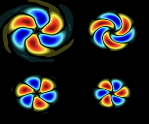
The explanation for the larger gain separation and clearer dominance of the streak mechanism comes from the larger phase velocities, and smaller associated streamwise wavenumbers, in the flight stream case. Strictly speaking, streaky structures are characterised by zero streamwise wavenumbers, developing parallel to the jet axis. This is the case at $St=0$. For small, but non-zero frequencies, the flow structures have non-zero streamwise wavenumbers (in which case they become helical), but they still bear most of the characteristics of streaks (Pickering et al. Reference Pickering, Rigas, Nogueira, Cavalieri, Schmidt and Colonius2020). However, they acquire an azimuthal phase velocity, $U_\theta = \omega /m$, which makes them rotate slightly around the jet axis as they evolve downstream. This can be seen in figure 15, which shows a cross-plane cut, made at $x/x_c =2.5$, of $m=3$ SPOD and resolvent modes at $St=0.02$. Resolvent modes computed at $St=0$ are also shown for comparison. In the flight stream case, the streamwise phase velocity, $U_c = \omega /\alpha$, with $\alpha$ the streamwise wavenumber, at a given frequency is higher. The higher phase velocity induces a smaller streamwise wavenumber of the associated structures, which has a direct impact on the gain separation. This can be demonstrated using a locally parallel model, which takes $\alpha$ as input. In Appendix D we use the model explored by Maia et al. (Reference Maia, Brès, Lesshafft and Jordan2023) to show that, at $St=0$, reducing the wavenumber indeed leads to a higher non-normality/gain separation. This agrees with the results obtained in the global analyses and explains the better agreement with SPOD modes in the flight stream case. Furthermore, the total phase velocity, given as the sum of the azimuthal and streamwise component, is more aligned with the streamwise direction in flight conditions. Note how, in figure 15, the rotation/swirling effect is much less marked with the flight stream. Besides from being more aligned with the jet axis, coherent structures in flight are also underpinned by a clearer signature of the lift-up mechanism, as discussed above. This makes them more similar to ‘classic’ $\omega =0$, $\alpha =0$ streaks.

Figure 15.

Cross-plane cut of leading SPOD and resolvent modes at $m=3$ and taken at $x/x_c=2.5$. The real part of the streamwise velocity modes are shown, with contours scaled to $\pm \|u_{x}\|$. (a) Static case, $M_f=0$, (b) flight case, $M_f=0.15$.