1. INTRODUCTION
With the development of intelligent technology, the application of unmanned surface vessels (USVs) in ocean surveying, rescue, patrol and other fields has become more and more extensive, and the related research is becoming more and more mature, mainly focusing on unmanned vessel control, tracking navigation, obstacle avoidance navigation, formation navigation and so on. Thus, at present, obstacle avoidance is one of the most important problems in research. Obstacle avoidance navigation is also, in essence, a path selection problem, and the goal of solving the problem is to realise the optimal obstacle avoidance path at the least cost. So, according to the different levels of understanding of the environment, obstacle avoidance planning can be divided into two types: global planning and local planning.
Global planning involves finding the appropriate path from the starting point to the final point according to a certain search algorithm after fully grasping the environmental information. The common methods are the visual graph method, probabilistic path map method, grid method and so on (Hong and Park, Reference Hong and Park2011; Yao et al., Reference Yao, Wang and Ji2017), which are usually used to construct an obstacle avoidance plan with the obstacle layout being obtained in advance. Considering the rules of collision avoidance at sea, Naeem et al. (Reference Naeem, Irwin and Yang2012) set up the geometric region to divide the obstacle avoidance zone by using global map planning. The improved A* algorithm was used to carry out the obstacle avoidance planning of USV. In Sun (Reference Sun2018), the improved A* algorithm and the potential field grid method were combined to develop a two-level global programming algorithm to obtain the optimal path, with the dual aims of effective obstacle avoidance and shorter voyage distance. Sun (Reference Sun2017) adopted the global path planning algorithm based on the multi-class classification support vector machine (SVM), which independently selected the parameter indices of path smoothness and obstacle distance in each bisector, and combined them with the kernel function method to complete path planning based on the binary SVM. Zhang (Reference Zhang2008) designed the global path planning of a USV using a genetic algorithm and artificial potential field method, which can plan for a variety of complex obstacle environments, and has the ability to find the optimal path in a three-sided obstacle environment around the starting point. Shi et al. (Reference Shi, Su and Zhang2018) used satellite remote sensing imagery to monitor the obstacle map, and then applied graph theory to plan the path. Wang et al. (Reference Wang, Yao and Dou2019) improved the wolf swarm algorithm to optimise the maximum expected programming function and obtained the optimal obstacle avoidance path.
However, global planning is not suitable for dealing with dynamic or sudden obstacle targets, and it needs to obtain enough environmental information to predict the next action (Zhu and Zhong, Reference Zhu and Zhong2010; Raja and Pugazhenthi, Reference Raja and Pugazhenthi2012; González et al., Reference González, Pérez, Milanés and Nashashibi2016). In fact, it is often faced with an unknown unstructured environment. The difficulties of obstacle avoidance navigation are strengthened due to the (in)ability to acquire environmental information and real-time requirements. Therefore, local planning has become the primary choice for autonomous obstacle avoidance navigation, and the corresponding real-time obstacle avoidance model has also been developed. Some research focuses on the establishment of a geometric region model to obtain an obstacle avoidance model. For unknown obstacle information, Wu et al. (Reference Wu, Xiong and Wen2014) considered the influence of wind and current on the manoeuvring characteristics of an unmanned aerial vehicle (UAV), analysed the model of relative velocity and relative position between UAV and obstacle, and realised the avoidance of a dynamic obstacle through change in the direction of movement. Zhu et al. (Reference Zhu, Cheng and Yuan2016) proposed a constraint reference frame to develop the potential field so that the decomposed forces can be matched with the physical constraints of the UAV for online adjustment. Pu et al. (Reference Pu, Feng and Li2017) put forward a predictable dynamic obstacle avoidance method for an unmanned submarine based on collision cone deduction, calculated the collision angle region for collision between an unmanned submarine and a dynamic obstacle, and obtained the collision angle of an unmanned submarine. Qu et al. (Reference Qu, Xing and Alexander2013) used the combination of a genetic algorithm and a geometric region obstacle avoidance model to design an obstacle avoidance strategy. Chen et al. (Reference Chen, Huang, Mou and van Gelder2018) designed a discrete-time nonlinear velocity obstacle avoidance method to predict the state of obstacle avoidance for a dynamic obstacle. Combined with devising collision avoidance rules, collision avoidance planning in a multi-obstacle environment was carried out and the idea of tracking was introduced into obstacle avoidance in Zhang et al. (Reference Zhang, Deng, Zhang and Huang2018). Song et al. (Reference Song, Su, Dong, Shen, Xiang and Mao2018) divided the problem of dynamic target obstacle avoidance planning into two levels, the first of which used the speed obstacle avoidance algorithm, and the second established the improved artificial potential field algorithm. The two levels were combined to adjust the speed and direction of the unmanned vessel. A proper penalty function field has been proposed in Lee et al. (Reference Lee, Parka and Eun2018) to be optimal collision-free transfers in real time, improving the efficiency of the obstacle avoidance model.
Some workers have paid attention to adaptive prediction and feedback learning for enhancing the performance of obstacle avoidance. Zhao et al. (Reference Zhao, Li and Shi2016) used a neural network to design a collision avoidance model for evaluating the collision situation. The work of Kozynchenkoa and Kozynchenko (Reference Kozynchenkoa and Kozynchenko2018) was specially designed for a ships crossing scenario using dynamic predictive programming based on a neural network and fuzzy algorithm. Zhang et al. (Reference Zhang, Tang, Su, Li, Yang and Shi2014) proposed an adaptive risk aversion decision model using the Sarsa (state–action–reward–state–action) online strategy reinforcement learning algorithm, and combined this with a progressive corruption algorithm as a behaviour exploration strategy. Wang et al. (Reference Wang, Zhang and Zhang2018) established a Markov decision-making method through reinforcement learning, and then the optimal strategy was solved by value function programming and simulated in static and dynamic obstacle environments. The deep reinforcement learning was also applied to train ships to avoid obstacles automatically (Shen et al., Reference Shen, Hashimoto, Matsuda, Taniguchi, Terada and Guo2019).
At present, from the simple geometric collision region determination model to the non-linear uncertainty prediction model, from offline learning to online real-time learning, most research increases the structure and judgment complexity of an obstacle avoidance algorithm or model in order to ensure the real-time performance of obstacle avoidance. Therefore, this paper considers reducing the complexity of the obstacle avoidance strategy model, to design a new obstacle avoidance algorithm for ensuring real-time requirements and simplifying the processing model, which can achieve the purpose of autonomous obstacle avoidance. This approach is believed to have the following advantages over existing solutions: (1) The grid cell activation model is constructed by using the bio-grid cell heuristic algorithm to simplify the model describing the distance relationship between the USV and the obstacle. (2) Considering the uncertainty, the dynamic expectation evaluation function is designed from the viewpoint of probability, which refers to the target orientation and decreases the spatial execution dimension, especially in the face of an unknown and complex environment.
The rest of the paper is organised as follows. In Section 2, the problem description is given. Section 3 presents the detailed design algorithm for obstacle avoidance. Simulation experiments under different obstacle scenarios are given in Section 4. Finally, the paper concludes in Section 5.
2. PROBLEM DESCRIPTION
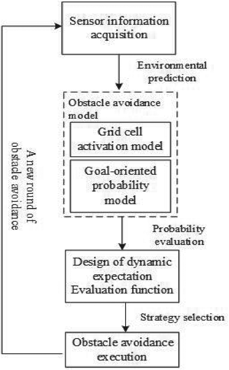
We consider that a USV will sail to designated target locations in multi-obstacle unknown environments, focusing on two main areas: (1) acquisition of environmental information, and (2) goal-oriented obstacle avoidance planning. Owing to the fact that this is real-time obstacle avoidance in the face of a locally known situation, it is not necessary to know all the environmental information, but only to make judgments on the basis of the information obtained from the actual sensors, and to establish a model to describe the distance between the USV and the obstacle. In order to reduce the complexity of the model, the grid cell activation model in bionics is combined to simplify the obstacle avoidance model. Meanwhile, aiming at the specified target location, the dynamic expectation evaluation function, including reward and punishment factors, is constructed to evaluate the optimal obstacle avoidance decision, through a design initialisation and update strategy, to reduce the judgment dimension, and to quickly obtain the execution decision for guaranteeing the real-time requirement. The overall process is shown in Figure 1.
Overall process of the obstacle avoidance algorithm.

3. DESIGN OF OBSTACLE AVOIDANCE ALGORITHM
3.1. The grid cell activation model
A large number of neurophysiological studies (O'Keefe and Nadel, Reference O'Keefe and Nadel1978; David and Pierre, Reference David and Pierre2006; van Strien et al., Reference van Strien, Cappaert and Witter2009) have shown that, in animals, the hippocampal formation in the brain is the part of the body mainly responsible for environmental cognition. Animals are able to use self-motion cues to maintain vector relationships relative to environmentally important positions, and to compute and integrate the information of each site in space so that this vector relationship is constantly updated. This process is dominated by grid cells in the entorhinal cortex of the hippocampus (Solstad et al., Reference Solstad, Moser and Einevoll2006; Witter and Moser, Reference Witter and Moser2006). Through the external discharge of the grid cells, the brain can continuously integrate the space angle and linear distance to locate the coordinates of its own environment for understanding its specific position in its surroundings. At present, the grid cell model theory is mostly used in autonomous positioning (Wei and Loo, Reference Wei and Loo2018; Yu et al., Reference Yu, Yuan and Li2018) and position navigation (Antonelo et al., Reference Antonelo, Schrauwen and Campenhout2007; Zhou and Wu, Reference Zhou and Wu2017). So, here, we use the grid cell model to describe the distance correlation between a USV and obstacles, and to establish the relevant regional model for obstacle avoidance.
According to Yu et al. (Reference Yu, Fang, Luo, Yuan, Jiang and Cai2016), biological studies confirmed that the grid cell fields are distributed in a triangular structure, and each grid field uses three striped cells to design the discharge activity of the grid cells. Therefore, a grid cell model based on striped cells is constructed as follows.
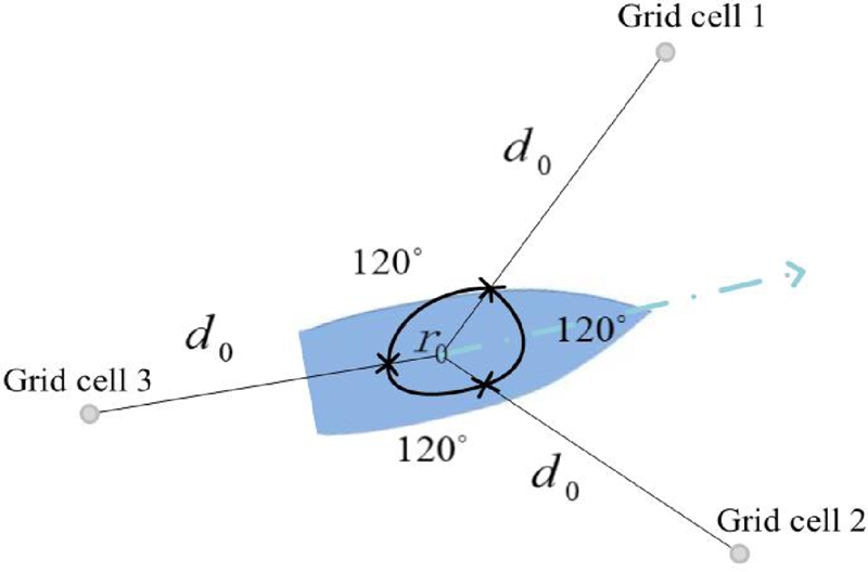
In Figure 2, a triangular obstacle avoidance model regarding grid cells is constructed by choosing the angles of  $60^{\circ }$,
 $180^{\circ }$ and
 $300^{\circ }$ clockwise along the heading direction and extending distance
 $d_{0}$ from the centre of the USV, instead of paying attention to all the ship perimeter information from the perspective of
 $360^{\circ }$. The triangular endpoint formed by the extension end is thought of as the grid cell, while the USV is in a position where it needs to be activated by its discharge. Viewing the grid cell activation model, the activation function of a single grid cell can be expressed as
 \begin{equation} g(r)=\tfrac{2}{3}(\phi(r)+\tfrac{1}{2}),\end{equation}
where  $\phi (r)=\frac {1}{3}\sum _{i}\cos (k_{i}(r-r_{0}))$ represents the discharge activity of each grid cell,
 $r$ is the position of the triangle endpoint (as shown by the small circle in Figure 2), which is determined by the detected distance between the obstacle and the USV along the direction of each grid cell, and
 $r_{0}=(x,y)$ is the position of the USV. Each grid cell is superimposed by three stripes with a difference of
 $60^{\circ }$ in the direction of the wavevector, where
 $i$ represents the number of the wavevector
 $(i=1,2,3)$ and
 $k_{i}$ represents the wavevector, as follows: (2).
 \begin{equation} \left\{\begin{array}{@{}l} k_{1}=\dfrac{4\pi}{\sqrt{6}\lambda} [\cos(\theta)+\sin(\theta),\ \cos(\theta)-\sin(\theta)], \\ k_{2}=\dfrac{4\pi}{\sqrt{6}\lambda} \left[\cos\left(\theta+\dfrac{\pi}{3}\right)+\sin\left(\theta+\dfrac{\pi}{3}\right),\ \cos\left(\theta+\dfrac{\pi}{3}\right)-\sin\left(\theta+\dfrac{\pi}{3}\right)\right],\\ k_{3}=\dfrac{4\pi}{\sqrt{6}\lambda} \left[\cos\left(\theta+\dfrac{2\pi}{3}\right)+\sin\left(\theta+\dfrac{2\pi}{3}\right),\ \cos\left(\theta+\dfrac{2\pi}{3}\right)-\sin\left(\theta+\dfrac{2\pi}{3}\right)\right],\end{array}\right. \end{equation}
where  $\lambda$ is the spacing between grid cells, and
 $\theta$ is the course of the USV.
Grid cell structure model.

For the grid cell activation model in Figure 2, which consists of three grid cells, the corresponding total activation probability function is
 \begin{equation} p_{c}(r)=\sum^{N}_{1}\omega_{n}g(r_{n}).\end{equation}
Here  $N$ is the total number of grid cells (
 $n=1,2,\ldots, N$);
 $g(r_{n})$ represents the activation rate of the
 $n$th grid cell at the spatial location
 $(x,y)$ in the environment facing obstacles, whose function is Equation (1); and
 $\omega _{n}$ represents the connection weight between the
 $nth$ grid cell and the discharge activation position, that is, the associated weight between the triangular endpoint formed by the extension end and the position of the USV (as shown in Figure 2), as follows:
 \begin{equation} \omega_{n}=\frac{4\pi\sigma^{2}}{3\lambda^{2}}\exp^{-4\sigma^{2}\pi^{2}/3\lambda^{2}},\end{equation}
with  $\sigma$ being the standard deviation parameter of the discharge activation domain.
Therefore, the grid cell activation model is employed to express the distance correlation between obstacles and the USV. The  $d_{0}$ value in the structure model of Figure 2 is set as the threshold value, and the distance information obtained from the sensor is used to judge the distance relationship between the obstacles and the USV. When any of the detected distances
 $d$ along the direction of the three grid cells (
 $r$ also changes with it) is less than the threshold value, the activation probability function of Equation (3) is triggered and gains the activation probability.
3.2. The goal-oriented probability model
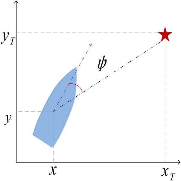
In order to reach the expected position as soon as possible, when planning the obstacle avoidance strategy, it should consider the expected goal-oriented path model. Here the course angle of the USV is used as a reference index to establish the goal-oriented model:
 \begin{equation} \psi=\theta-\arctan\left(\frac{y_{T}-y}{x_{T}-x}\right).\end{equation}
Equation (5) and Figure 3 are used to describe the extent to which the current course of the USV deviates from the situation of moving towards the target, where  $(x_{T},y_{T})$ is the intended target position. Then the Gaussian distribution function is used to find its probability; the maximum probability 1 means that the USV is sailing towards the expected target, indicating that the extent of deviation is 0. With the decrease of the probability, the extent of the deviation increases gradually:
 \begin{equation} p(\psi)=\exp\left\{ -\dfrac{1}{2}\left[\theta -\arctan\left(\dfrac{y_{T}-y}{x_{T}-x}\right)\right]^{2} \right\}.\end{equation}
Therefore, choosing the obstacle avoidance strategy always takes account of the intended target, by which path redundancy can be effectively avoided.
Goal-oriented structural model.

3.3. Dynamic expectation evaluation function
Combined with the above-mentioned grid cell activation model and the goal-oriented probability model, the positive-loss-rate expectation evaluation function is designed to find the maximum probability value of the possible obstacle avoidance strategy, and then the strategy selection and execution are carried out.
The positive-loss-rate expectation evaluation function is established under the condition of the maximum expected profit, and consists of the following evaluation function:
 \begin{equation} f_{\textrm{max}}=\text{correct rate} \times \text{reward factor loss rate} \times \text{punishment factor}.\end{equation}
The correct rate describes the probability proportion of the three grid cell directions in the grid cell activation model, which is expressed by  $({p_{c1}}/{p_{cm}},\ {p_{c2}}/{p_{cm}},\ {p_{c3}}/{p_{cm}})$, where
 $(p_{c1},p_{c2},p_{c3})$ are the actual activation probabilities in the three detection directions calculated by Equation (3). Here
 $p_{cm}$ means that the activation probability is calculated by choosing the threshold value
 $d_{0}$. The correct rate decreases with the decrease of the detected distance
 $d$.
The reward factor is mainly used to express the proportional relationship between the threshold distance  $d_{0}$ for triggering obstacle avoidance and the distance
 $d$ actually detected. When the detected distance satisfies
 $d\geq d_{0}$, the reward factor in this direction is considered to be the largest, and 10 is selected as the standard. When the detected distance satisfies
 $d< d_{0}$, the corresponding reward factor is
 $(d/d_{0})\times 10$; if the detected distance
 $d$ is closer to
 $d_{0}$, the reward value is higher, otherwise it is lower. The reward factor encourages the whole model of USV to be above the threshold distance range and stay away from the obstacle area.
As for the loss rate, it mainly describes the deviation level from the expected target position during obstacle avoidance planning, which is described by the goal-oriented probability model and expressed by  $1-p(\psi )$.
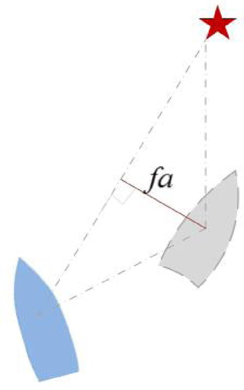
The punishment factor needs to combine the current state of the USV with the state of the next obstacle avoidance selection, and describes the deviation distance caused by the expected obstacle avoidance selection, as shown in Figure 4. The punishment factor corresponds to the loss rate, when the deviation level is large. The punishment factor is high, considering the timeliness and orientation, to avoid this kind of choice as far as possible.
Schematic diagram of punishment factor.

According to Figure 4, the result is
 \begin{equation} fa=|k_{0}x_{f}-y_{f}+y_{T}-k_{0}x_{T}|/\sqrt{k_{0}^{2}+1},\end{equation}
where  $k_{0}=\frac {(y_{T}-y)}{(x_{T}-x)}(x_{f},y_{f})$ is the next obstacle avoidance option position of the USV.
Therefore, according to the above process, the maximum value of the expected evaluation function in Equation (7) is solved. The corresponding obstacle avoidance selection when solving the maximum expectation is executed as an actual obstacle avoidance strategy.
Moreover, in order to enhance the computational efficiency, the midline is drawn from the vertex of the triangle which is composed of the endpoints of the actual detected distance in the two detection directions of the grid cell activation model: the grid cell 1 and the grid cell 2, and the centre of the unmanned ship. The angle of transition when the current course of the USV is turned to the midline direction is taken as the adjustment angle of the initial state. Equation (9) performs a status update mode until the maximum evaluation expectation is determined:
 \begin{equation} \theta_{\Delta}=\beta_{1}\theta+\beta_{2}\arctan\left(\frac{y_{T}-y}{x_{T}-x}\right),\end{equation}
where  $\beta _{1}$ and
 $\beta _{2}$ are gain parameters.
So, the obstacle avoidance algorithm has been constructed through Sections 3.1 to 3.3. It gives the optimal obstacle avoidance strategy for real-time planning. However, there is an obstacle avoidance situation that requires special treatment, referring to the following section.
3.4. Virtual obstacle model
What is involved above is a strategy to initiate obstacle avoidance action when the detected distance reaches the threshold distance value, but, in practice, the USV cannot be treated as a particle and needs to set up its own collision region. Once this region is entered, collision occurs, which should be avoided. For obstacle avoidance in a multi-obstacle environment, there is no way to know the global information in advance, so it is hard to predict whether it can pass safely or not. If the USV cannot pass through its own set collision region, it will choose a round-trip detour. While the USV only relies on the current situation and has no historical memory when choosing the strategy, it will cause this impassable state to happen again and again, leading to its sailing back and forth. Therefore, in order to break the continuous circulation of the special situation, it is necessary to add memory to the obstacle avoidance strategy, to avoid the recurrence of the previous impassable situation. In this paper, a virtual obstacle model is established to solve this kind of phenomenon.
When facing the fact that, no matter how the next strategy is chosen, the USV will finally enter its own collision area, which makes it impossible to proceed forwards and always to choose a round trip, it is necessary to take the position of the USV at that moment as the centre of a circle, to create a virtual circular obstacle of radius  $R$ and document it. Then, in the implementation of the following strategy, taking this virtual circular obstacle as an actual obstacle, it continues to deal with the judgment according to the above designed obstacle avoidance algorithm, which can avoid the occurrence of back-and-forth situations.
4. SIMULATION VERIFICATION
Here we assume that the initial position of the USV is  $(0,0)$, the initial course is
 $90^{\circ }$, the expected target position is
 $(50,120)$, the threshold distance value is
 $d_{0}=10$, and the parameters are
 $\sigma =0{\cdot }5$,
 $\beta _{1}=1$ and
 $\beta _{2}=0{\cdot }2$. The obstacle avoidance scene is composed of several static circular obstacles, which is simulated and demonstrated by using the MATLAB software platform.
The kinematic model is as follows:
 \begin{equation} \left\{\begin{array}{@{}l} \dot{x} = u\cos\theta-v\sin\theta, \\ \dot{y} = u\sin\theta+v\cos\theta, \\ \dot{\theta} = r_{\theta},\end{array}\right. \end{equation}
where  $u$,
 $v$ and
 $r_{\theta }$ are the velocities in the surge, sway and yaw directions, respectively. Here, any external interference is ignored, the default
 $v\approx 0$, and we choose
 $u=2$.
4.1. Comparative analysis of two obstacle avoidance algorithms
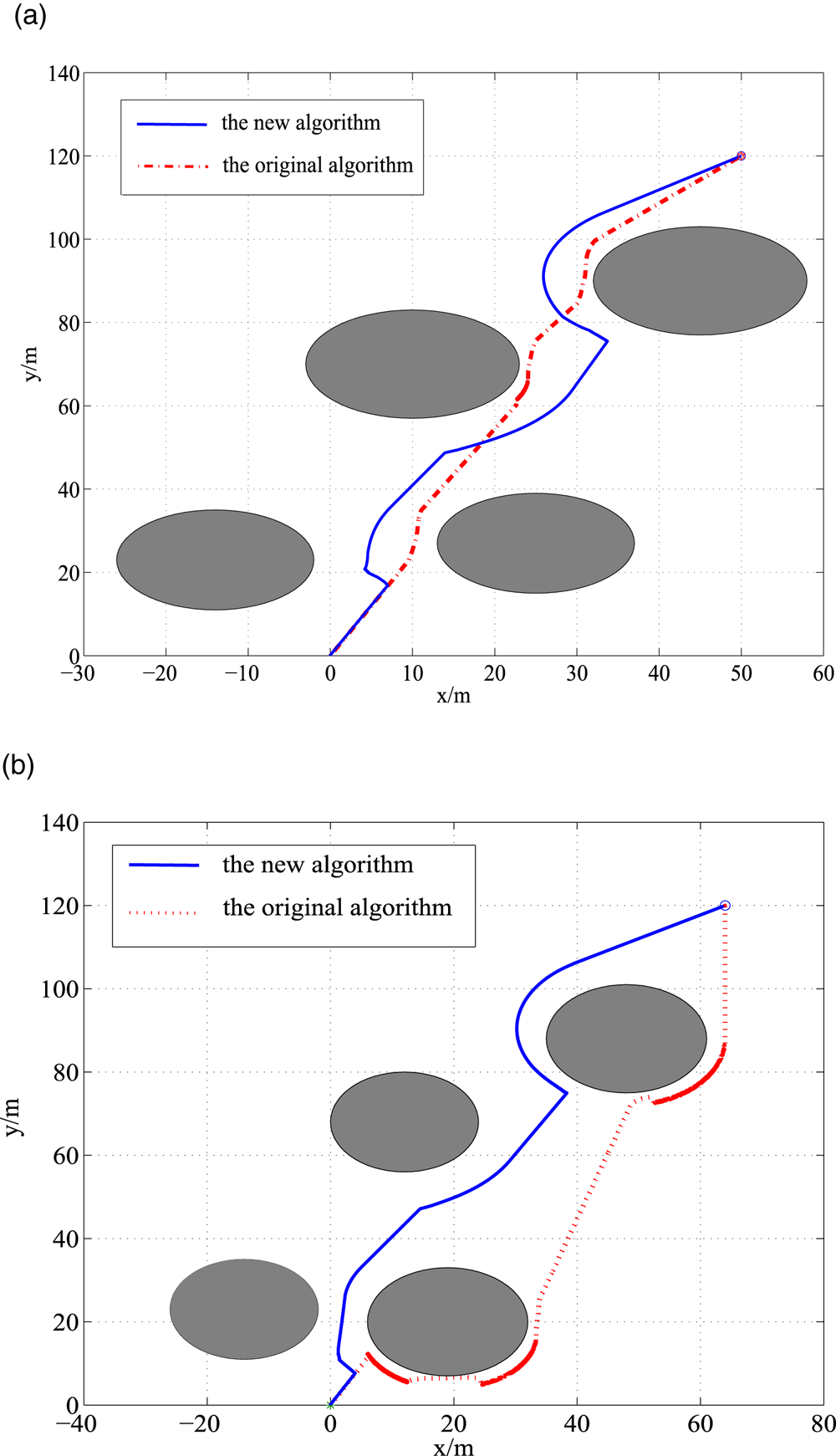
According to Figure 5, the blue solid line is the algorithm designed in this paper, and the red dotted line is the obstacle avoidance planning using the artificial potential field algorithm. Through comparative analysis, it is concluded that each of the two algorithms has its own advantages and can achieve the target smoothly; the USV sails directly towards the target at the beginning, and adjusts the course angle to avoid the obstacle when encountering obstacles until it reaches the desired goal.
Effect of obstacle avoidance under two algorithms.

However, the algorithm designed in this paper is more suitable for the comprehensive evaluation of multi-obstacle environments, and is superior to the improved potential field algorithm in unknown environments. The original artificial potential field algorithm focuses on the obstacle avoidance of a single obstacle, and the planning effect does not perform well when increasing the change of obstacles layout or when the distance among obstacles becomes short. However, the new algorithm has some large turns that ensure the safety of sailing, and no closer to the obstacles than that of the original algorithm. Therefore, this proposed new algorithm can effectively achieve obstacle avoidance with good performance in the running ability and complex obstacle environment.
4.2. Simulation of obstacle avoidance under different obstacle layouts
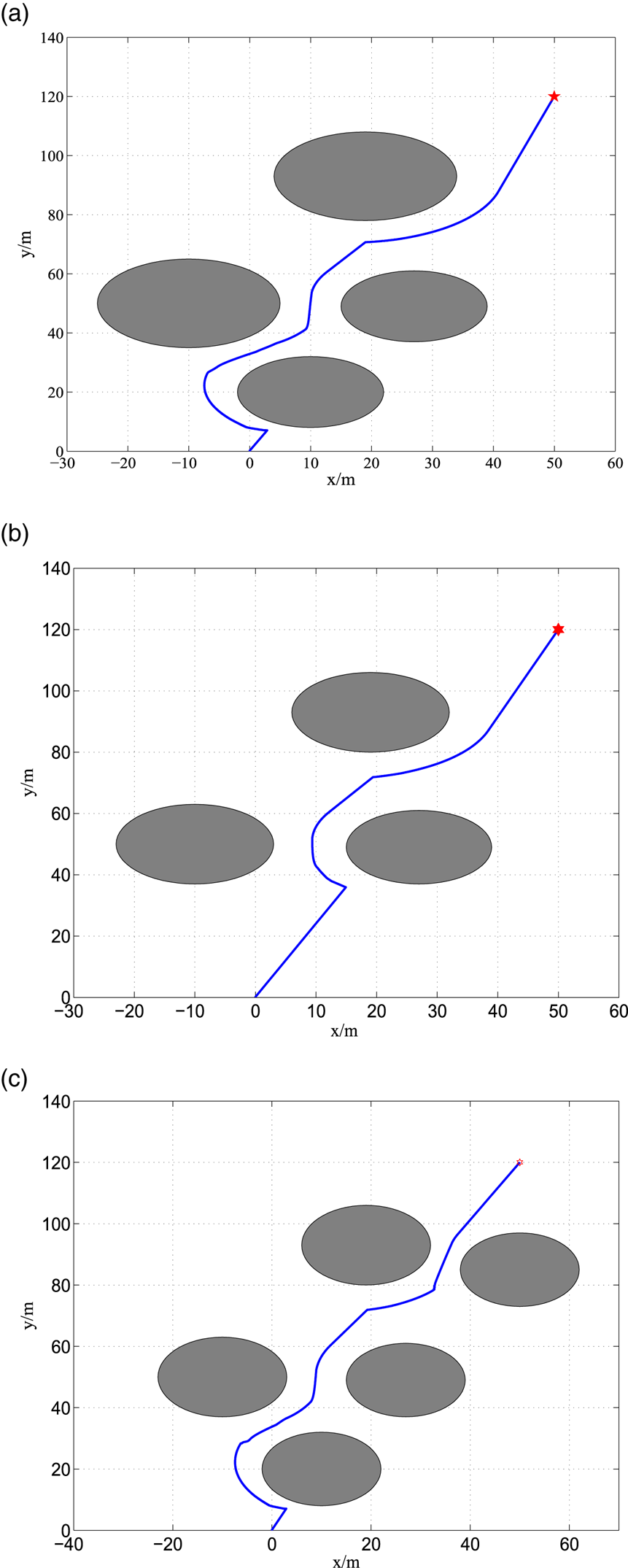
According to the obstacle avoidance procedure in Section 2, the real-time obstacle avoidance strategy of the USV is carried out and verified in different obstacle position layouts. From Figures 5 and 6, it can be concluded that the USV has successfully evaded the obstacles to reach the desired position, and the trajectory is basically smooth, but, in some places, one can clearly view places with large turns. This is mainly due to the need to ensure navigation towards the target, and is also necessary to avoid collision obstacles simultaneously, resulting from their combined effect.
Effect of obstacle avoidance under different obstacle layouts.

Compared with Figure 5, the obstacle location in Figure 6(a) is different, which results in a different path for obstacle avoidance. It selects the best strategy according to the expected maximum evaluation function, to find the appropriate way to avoid obstacles. Figure 6(b) and 6(c) are obstacle avoidance scenarios formed by decreasing and increasing the number of obstacles on the basis of Figure 6(a), respectively. Due to the difference in the number of obstacles, different obstacle avoidance paths are obtained according to the evaluation algorithm.
In the above, the obstacle avoidance path is affected by the expected target and the number and location of obstacles encountered along the way, resulting in different planning trajectories. According to the obstacle avoidance algorithm, the decision on the surrounding obstacle environment can be made in real time, choosing the appropriate obstacle avoidance path, and successfully completing navigation to the target.
4.3. Simulation of obstacle avoidance in the case of an impassable situation
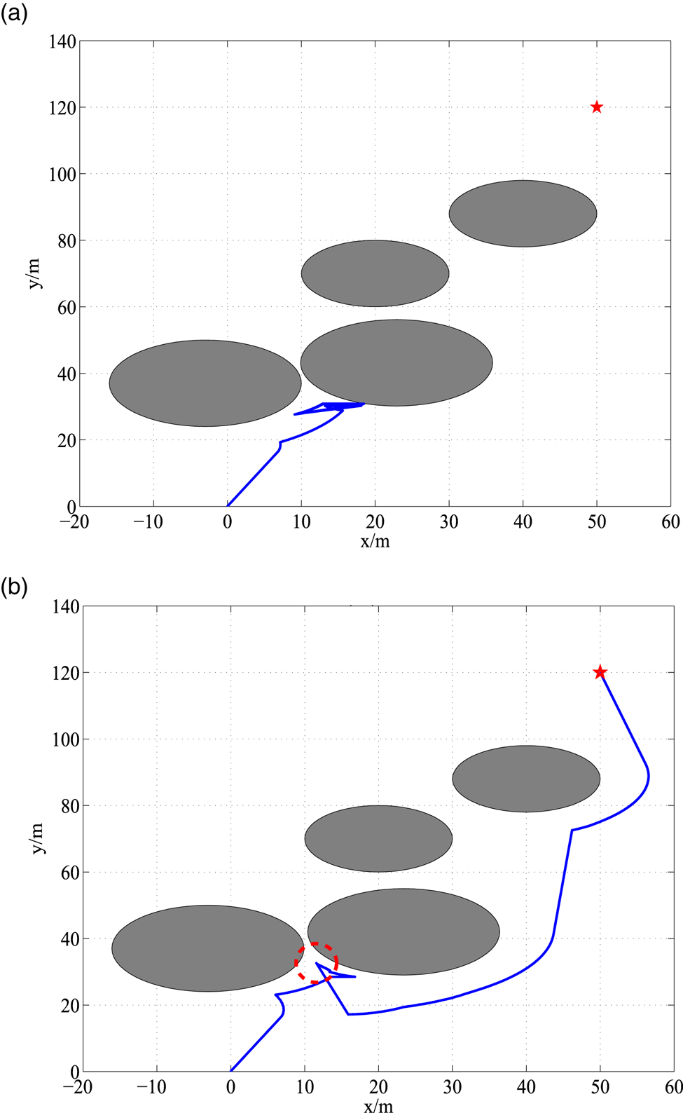
Under a multi-obstacle layout, for adjacent relatively close obstacles, the USV cannot pass and will choose to sail back, but due to the influence of goal guidance, it may also choose to turn back and forth again, resulting in the effect of a round trip. To avoid this particular situation, it creates a virtual obstacle model to avoid it. According to Figure 7(a), there is no virtual obstacle, causing the phenomenon of stagnating back and forth, which affects normal navigation. But the virtual obstacle avoidance model is adopted in Figure 7(b), and the circle represented by the red dotted line is the virtual obstacle, which is recorded as an actual obstacle, to be conducive for the later strategy choice, and the back-and-forth phenomenon is successfully avoided when encountering the round trip.
Effect of obstacle avoidance with and without a virtual obstacle.

Therefore, through the above argumentation and analysis, it is shown that the real-time obstacle avoidance method designed in this paper can achieve obstacle avoidance navigation very well in the complex environment with multiple obstacles, and can also effectively avoid the special back-and-forth phenomenon.
5. CONCLUSION
Using bionics for reference, this paper constructs an obstacle avoidance method combining the grid cell activation model and the goal-oriented probability model, and designs a positive-loss-rate expectation evaluation function to optimise the obstacle avoidance strategy, considering the reduction of execution complexity, where the structure of obstacles is ignored, and it is not necessary to know the surrounding environment information in advance. The later verification results are good, and there is a smooth and reasonable obstacle avoidance trajectory, which has a simplified structure, meets the real-time requirements and effectively solves the real-time obstacle avoidance problem in a multi-obstacle environment. However, this paper does not deal with the impact of a dynamic obstacle, and the lack of ship manoeuvrability, and, in addition, the large turns in the path should be weakened for further consideration in actual situations; it is necessary to further explore all of these in the future.
ACKNOWLEDGMENTS
This work is supported by the National Natural Science Foundation of China under Grants Nos. 51909155 and 51709166.