1.1 A Brief History of the Geometric Optics Method for Light-Scattering Calculations
Knowledge of light scattering by particles is inevitably necessary for numerous disciplines, including astrophysics, planetary sciences, bio-optics, radiative transfer, remote sensing, climate science, and a wide range of subjects covered by applied optics. In the case of spherical particles, the rigorous Lorenz–Mie theory has been well established (Lorenz, Reference Lorenz1890; Mie, Reference Mie1908). Of particular note is that the theory for light scattering by a sphere is usually referred to as the Mie theory, without giving appropriate credit to Ludvig Valentin Lorenz (1829–1891) for his pioneering work in this regard. For fairness from the historical perspective, it has been advocated that the theory of light scattering by a sphere be called the Lorenz–Mie theory (Kragh, Reference Kragh1991). Early studies of the scattering of plane waves by spheres were reviewed by Logan (Reference Logan1965). More recently, a volume edited by Hergert and Wriedt (Reference Hergert and Wriedt2012) is dedicated to a comprehensive review of the history of the Lorenz–Mie theory and its extensions. Although the Lorenz–Mie theory is regarded as a solved problem in classical physics, some fascinating new features associated with light scattering by a sphere were discovered in the twentieth and twenty-first centuries, such as the narrow resonance structure in the Lorenz–Mie scattering characteristics (Chýlek et al., Reference Chýlek, Kiehl and Ko1978) and the zero-backscattering of a sphere when the particle’s relative impedance with respect to the counterpart of the ambient medium is unity (Zhai et al., Reference Zhai2008).
Historically, light-scattering computations based on the Lorenz–Mie theory were challenging because of numerical instability, particularly in the case of an absorptive sphere. Fortunately, numerical stability has been achieved through the utilization of a downward recurrency scheme in light-scattering computation based on the Lorenz–Mie theory, as reported by Kattawar and Plass (Reference Kattawar and Plass1967). Furthermore, we call special attention to a milestone contribution made by Wiscombe (Reference Wiscombe1980) for the computational convergence and efficiency in the numerical implementation of the Lorenz–Mie theory. With various robust open-access computational programs based on the Lorenz–Mie theory, it is now regarded as a trivial effort to compute the optical properties of a sphere of essentially any practical size, ranging from the Rayleigh regime (the particle size is much smaller than the wavelength of the incident light) to the geometric optics regime (the particle size is much larger than the wavelength of the incident light). In particular, special software was already developed for the Lorenz–Mie computation using a mobile phone even in the 2000s (Wriedt, Reference Wriedt2008).
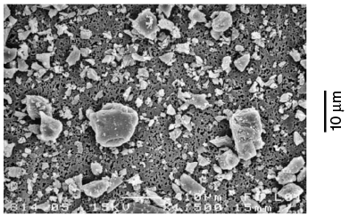
Despite the success in dealing with the scattering of light by a sphere based on the Lorenz–Mie theory, many particles in nature or those generated in laboratories, such as ice crystals in cirrus clouds, airborne dust aerosol particles in the atmosphere, interstellar dust particles, many oceanic particles, and artificial dust aerosol particles, are nonspherical. For example, Figure 1.1 shows the scanning electron microscope (SEM) images of feldspar particles that have various irregular shapes. These particles were generated by crushing large rocks (Volten et al., Reference Volten2005). It is highly unlikely to account for the morphological details of these particles in light-scattering computation. As a first-order approximation, the spheroid model has often been used to account for the nonsphericity effects in downstream applications in remote sensing of dust aerosol properties. The spheroid model represents a significant improvement compared to the sphere model because the spheroidal geometry has two degrees of freedom (i.e., particle’s maximum dimension and the aspect ratio, which is the ratio of particle’s major axis to its minor axis), whereas spherical geometry has only one degree of freedom (i.e., particle size).
SEM image of feldspar particles. The particles are highly irregular in shape and show considerable differences in size. The scale of the illustration is indicated by the vertical bar on the right.
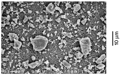
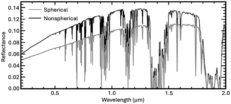
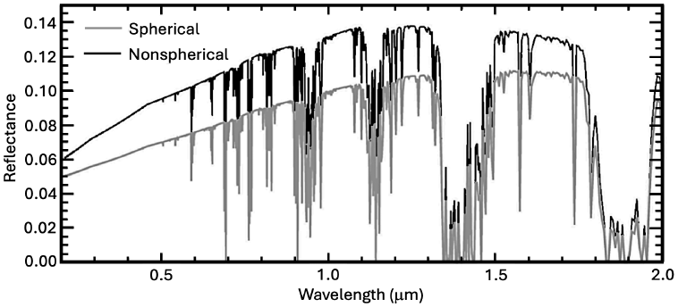
Figure 1.2 demonstrates the impact of a particle’s nonsphericity on the atmospheric radiation field and shows two solar reflectance spectra at the top of the atmosphere (TOA), which are simulated with the US standard atmosphere for an overcast, dusty sky. The upper and lower spectral curves in Figure 1.2 correspond to using the spheroid and sphere models, respectively. For the simulations, the solar zenith angle is 60° and the viewing angle is 0°, the aerosol optical depth (AOD) of the dust layer is 1.0 at a wavelength of 0.55 µm, and the surface albedo is 0.1. It can be seen from Figure 1.2 that neglecting the nonsphericity of dust particles can significantly underestimate the TOA reflectance. This underestimation has an important implication for assessing the radiative forcing effect of airborne dust, which is an important factor involved in climate studies.
Simulated solar reflectance spectra from 0.2 to 2.0 microns at the top of the atmosphere under overcast, dusty sky conditions with spherical and nonspherical (specifically, spheroidal) particles.
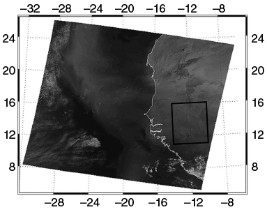
To demonstrate the effect of a particle’s nonsphericity on remote sensing of dust aerosol properties from spaceborne observations, we select a scene observed by the Moderate Resolution Imaging Spectroradiometer (MODIS) on the Terra satellite (King et al., Reference King1992) over West Africa on March 2, 2003. In particular, Figure 1.3 (Feng et al., Reference Feng2009) shows the RGB (R: band 1 covering from 620 to 670 nm; G: band 4 covering from 545 to 565 nm; and B: band 3 covering from 459 to 479 nm) false-color image based on MODIS observations. Dust transport from land to the ocean can be clearly seen in the image. The area indicated by the rectangular box is selected for the inference of dust AOD.
MODIS RGB image on March 2, 2003, showing a dust plume over West Africa. The area indicated by the small box is used to retrieve dust AOD.
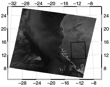
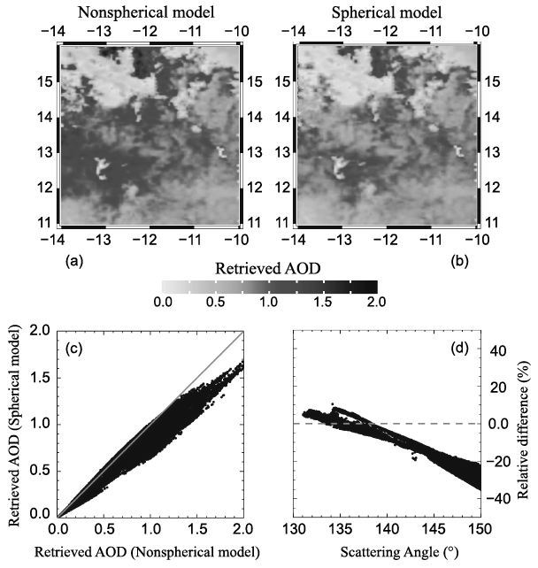
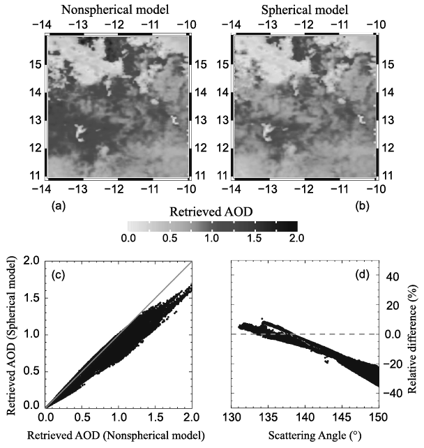
Figure 1.4a,b shows the dust AOD retrievals for the area indicated by the small box in Figure 1.3, for which nonspherical (spheroidal) and spherical dust models are assumed, respectively. From the comparisons shown in Figure 1.4c,d, it can be seen that the impact of dust particle nonsphericity on the inferred dust AOD is significant, particularly for those pixels corresponding to scattering angles larger than ~140°. Moreover, in an earlier study, Dubovik et al. (Reference Dubovik2006) showed that using the sphere model may result in an erroneous fine mode in the retrieved aerosol size distribution and a spurious spectral variation of the real part of the refractive index in the visible wavelength regime, as demonstrated by remote sensing of aerosol properties from the ground-based radiometric measurements provided by the AERosol Robotic NETwork (AERONET) (Holben et al., Reference Holben1998). These studies (Dubovik et al., Reference Dubovik2006; Feng et al., Reference Feng2009) show that it is necessary to consider particle nonsphericity for spaceborne and ground-based remote-sensing implementation.
(a)–(b) The retrieved dust AOD values based on the spheroid (a) and sphere (b) models. (c) Retrieved dust AOD based on the sphere model versus the counterpart based on the spheroid model. (d) The relative differences between the AOD retrievals based on the spheroid and sphere models, with the former as the benchmark.
Although the nonsphericity effect of scattering particles is critical to many applications, computing the optical properties of a nonspherical particle poses a significant challenge, particularly from the perspective of numerical computation (Mishchenko et al., Reference Mishchenko, Hovenier and Travis2000). Exact methods include the method of separation of variables, which in practice is applied only to regular geometries, such as spheroidal particles (Oguchi, Reference Oguchi1973; Asano and Yamamoto, Reference Asano and Yamamoto1975; Ding and Yang, Reference Ding and Yang2023), the T-matrix method implemented via the extended boundary condition approach (Waterman, Reference Waterman1965, Reference Waterman1971; Barber and Yeh, Reference Barber and Yeh1975; Tsang et al., Reference Tsang, Kong and Shin1985; Barber and Hill, Reference Barber and Hill1990; Mishchenko and Travis, Reference Mishchenko and Travis1994; Mishchenko et al., Reference Mishchenko, Travis and Mackowski1996; Doicu et al. Reference Doicu, Wriedt and Eremin2006), and the invariant imbedding T-matrix method (IITM) (Johnson, Reference Johnson1988; Bi et al., Reference Bi2013; Bi and Yang, Reference Bi and Yang2014a). Numerically feasible and robust methods, such as the finite-difference time domain (FDTD) method (Yee, Reference Yee1966; Yang and Liou, Reference Yang and Liou1996a; Sun et al., Reference Sun, Fu and Chen1999; Taflove and Hagness, Reference Taflove and Hagness2005) and the discrete dipole approximation (DDA) (Purcell and Pennypacker, Reference Purcell and Pennypacker1973; Draine and Flatau, Reference Draine and Flatau1994; Yurkin and Hoekstra, Reference Yurkin and Hoekstra2007), are usually applied to small-to-moderate-size particles in comparison with the wavelength of the incident electromagnetic wave. Moreover, these methods require considerable computational effort for moderate-size particles. Many nonspherical particles in nature, such as ice crystals and coarse-mode dust particles in the atmosphere and phytoplankton in the ocean, are much larger than visible wavelengths. In addition, it is necessary to consider particle orientations (usually random orientations) for many practical applications, and averaging particle optical properties over orientations substantially increases computational burden. To compute the optical properties of these particles at the aforementioned wavelengths, the only viable option is to employ the principles of geometric optics as an approximate method, with accuracy increasing as the particle size increases; in other words, the geometric optics method represents a case where there is “no alternative” for computing the optical properties of nonspherical particles that are much larger than the wavelength of the incident electromagnetic wave.
Classical optics has a long history. Born and Wolf (Reference Born and Wolf1999) and Strong (Reference Strong1958) briefly reviewed the milestones in the development of classical optics. Of the principles of classical optics, which were essentially fully developed before the twentieth century, in this book, we are mainly concerned with the concepts of a geometric optics “ray,” Snell’s law, the reflection and refraction of a ray, and Fraunhofer diffraction. The reason is that scattered light within the framework of classical optics is assumed to be a combination of classical diffraction and geometrical ray reflection and transmission (Hodkinson and Greenleaves, Reference Hodkinson and Greenleaves1963). It is not feasible for us to trace the origin of the concept of a ray. As articulated by Born and Wolf (Reference Born and Wolf1999), the concept of a ray can be well illustrated by thinking of the passage of collimated light through a tiny opening in an opaque screen, which, at first sight, illuminates a region with a sharp boundary. As we will explain in detail in Chapter 2, the validity of the ray concept actually depends on the cross section of the ray beam. Studies of basic ray or beam propagation, as explained by Strong (Reference Strong1958), can be traced to the effort of Euclid (~300 BC) describing ray reflection and of Ptolemy (AD 70-147) describing ray refraction. The law of refraction, which is known as Snell’s law, was attributed to the experimental work of Willebrord Snellius (c. 1580–1626) or Snell. It has been advocated that Snell’s law be called Snel’s law because of the original spelling of his name, Willebrord Snel van Royen (Adams and Kattawar, Reference Adams and Kattawar1997).
Light (and electromagnetic radiation in general) has a very complex nature, and scientific knowledge of the many phenomena associated with light has only gradually evolved over many centuries. Historically, light propagation was regarded as being in the form of minute particles, for example, by Newton. Thomas Young’s double-slit interference experiment conducted at the beginning of the nineteenth century played an instrumental role in the general acceptance of the wave theory of light, for which Robert Hooke (1635–1703) and Christiaan Huygens (1629–1695) were pioneers. In 1816, Augustin-Jean Fresnel (1788–1827) developed his theory of diffraction without considering polarization. In 1823, Fresnel derived formulas, which are now called Fresnel equations, for the amplitude, phase, and polarization of the transmitted and reflected waves. For a more in-depth study of the development of polarization of light, the reader is referred to Brosseau (Reference Brosseau1998).
The earliest quantitative applications of the principles of geometric optics to light scattering were developed for spherical particles. For example, Mecke (Reference Mecke1920) studied the scattering of light incident on a sphere by using the principles of geometric optics and the diffraction associated with a circular disc of the same radius as the sphere. He fully considered the phase of all rays. Bricard (Reference Bricard1946) suggested that, when  , where m is the index of refraction and x is the size parameter defined as 2
 times the ratio of particle radius to the wavelength of the incident light, the interference between contributions of the geometric optics rays and diffraction is essentially incoherent, and the two contributing components can be treated separately. It should be pointed out that, in classical geometric optics methods, the geometric optics rays and diffraction equally contribute to the total extinction. The extinction due to diffraction stems from the corrective field in the shadow region of a sphere illuminated by a collimated beam, as illustrated through a rigorous analysis by Brillouin (Reference Brillouin1949), who clarified some inconsistencies and misinterpretations found in several early texts regarding the fact that the extinction cross section is twice the geometric projected area in the case of light scattering by a large particle compared to the wavelength of incident light.
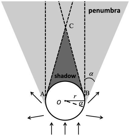
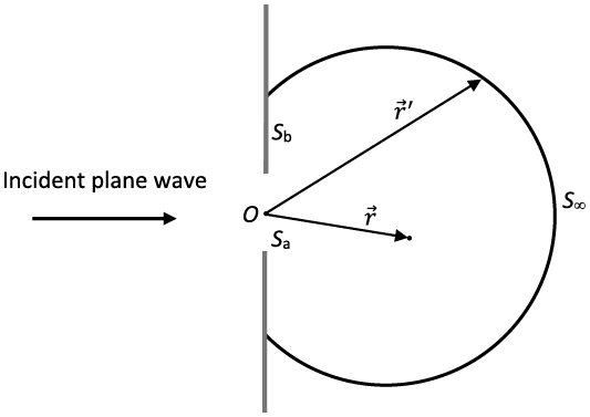
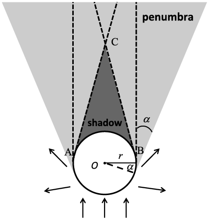
In the history of studying light scattering by large particles, there was intense debate as to whether the extinction efficiency (defined as the ratio of the extinction cross section to the geometric projected area of the particle) is always 2. To clarify the apparently dubious physical process, let us consider the scattering of light by a perfectly conducting sphere. In this case, since there is no absorption involved, the extinction efficiency equals the scattering efficiency (defined as the ratio of the scattering cross section to the geometric projected area of the particle). As shown in Figure 1.5, blocking of the incident light leads to a conical shadow region marked as ABC in the schematic diagram in Figure 1.5. Outside the shadow region, there is a penumbra region. Beyond the penumbra region, the scattered field is essentially given by the external reflection of the incident light by the sphere. With an increase in the ratio of particle size to the wavelength of the incident light, angle  in Figure 1.5 decreases, the shadow extends, and the penumbra shrinks. In the geometric optics limit (i.e., in the case of light scattering by a very large particle), it is assumed that angle is essentially zero and the blocking of the incident light leads to a cylindrical shadow region behind the sphere. The blocking of the incident light corresponds to electromagnetic radiation flux given by
 , where
 is the incident irradiance. Thus, the contribution to the extinction efficiency due to the blocking effect is 1. Furthermore, near the surface of the sphere within the shadow region, the total electric and magnetic fields are zero, given by
 (1.1.1a)
 (1.1.1b)
where superscripts t, i, and c indicate the total, incident, and corrective fields, respectively. Equations (1.1.1a) and (1.1.1b) indicate that the corrective field cancels the incident field. It is the corrective field that leads to an additional attenuation of the incident light with an amount of  . Thus, the total extinction efficiency is 2. The reader is referred to Brillouin (Reference Brillouin1949) for a detailed mathematical derivation of the contribution of the corrective fields to the extinction efficiency. The contribution of the corrective fields to the scattered fields is a physical phenomenon referred to as diffraction, which is fundamentally due to the incomplete wave front of a propagating wave. Section 1.5 provides a more detailed explanation of diffraction, particularly far-field diffraction, known as Fraunhofer diffraction (Born and Wolf, Reference Born and Wolf1999).
Schematic diagram illustrating the scattering of light by a perfectly reflective opaque sphere (i.e., a perfectly reflective sphere) within the geometric optics framework. Diagram concept based on Brillouin (Reference Brillouin1949).
Following the studies of Mecke (Reference Mecke1920), Bricard (Reference Bricard1946), and van de Hulst (Reference van de Hulst1957), Ellison and Peetz (Reference Ellison and Peetz1959) reported the forward scattering of light by spheres according to geometric optics. Hodkinson and Greenleaves (Reference Hodkinson and Greenleaves1963) also performed numerical computation of light scattering by a sphere using the geometric optics method for scattering angles up to 40º. They also compared the geometric optics results with the Lorenz–Mie solutions for size parameters up to 30. A comprehensive formalism of the light scattering by a sphere within the framework of geometric optics can be found in van de Hulst (Reference van de Hulst1957). Liou and Hansen (Reference Liou and Hansen1971) applied the geometric optics method to light scattering by polydisperse spheres (an ensemble of spheres with a distinct distribution of sizes) to compute the phase function and the degree of linear polarization. They compared the geometric optics method with the exact Lorenz–Mie theory and found that the two methods were in close agreement for real refractive indices m = 1.33 and 1.50 for an ensemble of polydisperse, homogeneous, and spherical particles when the effective particle size (Hansen and Travis, Reference Hansen and Travis1974) parameter is larger than approximately 100. At a size parameter of 400, the phase function results based on the geometric optics method converge to the Lorenz–Mie results, although the backscattering peak corresponding to an optical phenomenon known as the glory does not appear in the geometric optics solution in the case of m = 1.33, which is approximately the index of refraction of water at a visible wavelength, regardless of the size parameter.
Application of the geometric optics method has been extended to nonspherical particles, such as the scattering of light by spheroids (Lock, Reference Lock1996a,Reference Lockb). In particular, Lock (Reference Lock1996a) obtained a closed-form solution for diffraction and external reflection for an arbitrarily oriented spheroid. In the case of light scattering by a transparent spheroid, the curvature effect of the spheroidal surface poses a significant challenge for performing rigorous ray-tracing calculations. In particular, the equal-phase wavefront associated with the refracted rays is distorted in reference to that of the incident collimated beam (a bundle of rays) after passing through a curved surface. As a result, the cross-section of a beam with a curved wavefront during propagation in a homogeneous medium varies with the ray-bundle propagation distance. Moreover, the phase of a beam with a convergent wavefront undergoes a phase shift of π/2 with each passage of a focal line. The contribution to the scattering amplitude by a beam after passing over a scatterer is determined by three elements: the cross-section variation of its wavefront, the total wave phase, and the refraction coefficients determined by the Fresnel equations. Ren et al. (Reference Ren2011) and Sun et al. (Reference Sun2016) developed a complex vector ray model to overcome the difficulties encountered in considering the wavefront and wave phase in the case of light scattering by a spheroid.
The geometric optics method has been especially applied to light scattering by faceted particles (ice crystals with flat, smooth, polygonal faces), mainly due to the importance of ice clouds in atmospheric remote sensing and climate science. Ice crystals in the atmosphere are almost exclusively nonspherical particles (e.g., Heymsfield and Iaquinta, Reference Heymsfield and Iaquinta2000; Bailey and Hallett, Reference Bailey and Hallett2009), ranging from pristine plates and columns to highly irregular aggregates with small-scale irregularities and surface roughness. The earliest study of the optical properties of hexagonal ice crystals was conducted by Jacobowitz (Reference Jacobowitz1971), as part of the author’s PhD dissertation at Massachusetts Institute of Technology (MIT). In the 1980s and 1990s, the geometric optics method, by means of the ray-tracing technique, was extensively used to investigate the single-scattering properties of nonspherical ice crystals (Wendling et al., Reference Wendling, Wendling and Weickmann1979; Cai and Liou, Reference Cai and Liou1982; Takano and Jayaweera, Reference Takano and Jayaweera1985; Takano and Liou, Reference Takano and Liou1989; Macke, Reference Macke1993; Macke et al., Reference Macke, Mueller and Raschke1996). Using the Monte Carlo method, Wendling et al. (Reference Wendling, Wendling and Weickmann1979) might be the first to quantify the 22° and 46° halo peaks and a scattering maximum at 154° in the phase function of randomly oriented ice crystals. However, in the Wendling et al. (Reference Wendling, Wendling and Weickmann1979) study, diffraction by a hexagonal ice crystal is approximated by that of a rectangular aperture regardless of the orientation of the ice crystal; moreover, polarization is not included; consequently, their results are limited only to the phase function. Cai and Liou (Reference Cai and Liou1982) fully incorporated the polarization configuration and phase interference in the ray-tracing calculation for randomly oriented hexagonal ice crystals. They also rigorously considered the diffraction pattern associated with the projected area of a three-dimensional (3D) hexagonal particle. However, the phase matrix elements P33 and P44 reported by Cai and Liou (Reference Cai and Liou1982) are incorrect, which were later corrected by Takano and Jayaweera (Reference Takano and Jayaweera1985). The theoretical framework for the “conventional” geometric ray-tracing technique and the associated computational algorithm developed by Cai and Liou (Reference Cai and Liou1982) for hexagonal columns and plates were further improved and refined by a number of researchers. In particular, the single-scattering properties associated with more complex particle morphologies (Macke, Reference Macke1993; Macke et al., Reference Macke, Mueller and Raschke1996; Takano and Liou, Reference Takano and Liou1995; Yang and Liou, Reference Yang and Liou1998) have been studied with a similar methodology implemented with the Monte Carlo technique. Moreover, Takano and Liou (Reference Takano and Liou1989) incorporated the effects of birefringence of ice into the ray-tracing computation.
An innovative method was developed by Muinonen (Reference Muinonen1989) to improve the conventional ray-tracing method by employing a modified Kirchhoff approximation, which maps the near field obtained with the ray-tracing technique to the far field. In this form, the spread of a ray due to the phase interference can be accounted for. As a result, unlike the results given by the conventional ray tracing techniques, the scattering peaks associated with halos in the case of the scattering of visible light by a hexagonal ice crystal under the random orientation condition are not independent of the size parameter for the solution given by the modified Kirchhoff approximation approach. However, the modified Kirchhoff approximation approach developed by Muinonen (Reference Muinonen1989) separates the contributions of diffraction and the geometric rays in the same way as the conventional geometric optics method, by assuming that the extinction efficiency is 2 regardless of the size parameter. To overcome this shortcoming, the near field computed with the ray-tracing procedure with a full inclusion of the phase and the field polarization configuration can be mapped to the far field through an exact electromagnetic surface integral equation (Yang and Liou, Reference Yang and Liou1996b) or an exact electromagnetic volume integral equation (Yang and Liou, Reference Yang and Liou1997). The surface- and volume-integral-based methods produce consistent results, particularly for relatively large particles compared to the wavelength of the incident light (Yang et al., Reference Yang2019). To the best of our knowledge, these improvements for the first time capture the variations of the extinction efficiency as a function of the size parameter within the framework of the geometric optics method (Yang and Liou, Reference Yang and Liou1995), and this improvement is referred to as the physical-geometric optics method (PGOM). The singularity known as the delta-transmission (Takano and Liou, Reference Takano and Liou1989), inherent to the conventional ray-tracing calculation in the case of a scattering particle with parallel surface facets, is overcome by the aforementioned PGOM method. Furthermore, PGOM is applicable to a much wider size parameter range compared to the conventional geometric optics method, as demonstrated by Yang et al. (Reference Yang2019). The volume-integral approach can be numerically implemented in terms of a ray-by-ray integration (RBRI) technique (Yang and Liou, Reference Yang and Liou1997) that, unfortunately, is computationally inefficient. Bi et al. (Reference Bi2011) and Sun et al. (Reference Sun, Yang, Kattawar and Zhang2017b) further improved the RBRI technique by implementing simultaneous tracing of a bundle of rays (referred to as a beam) impinging on the same facet. In addition, an improved method referred to as the beam-splitting method (Bi et al., Reference Bi2011) in conjunction with computer graphics techniques (Sun et al., Reference Sun, Yang, Kattawar and Zhang2017b) has been developed for a faceted convex particle that may contain a core or an inclusion with a different refractive index (Sun et al., Reference Sun, Yang, Kattawar and Zhang2017b). Most recently, Yang et al. (Reference Yang2019) extended the previous work to concave particles, particularly aggregates, and a more efficient computational algorithm was developed to map the near field on a cubic surface enclosing the particle to the far field based on an exact electromagnetic surface-integral equation. A synergistically unified method (Yang and Kattawar, Reference Yang and Kattawar2023) based on combining IITM (for small-to-moderate-size parameters) and PGOM (for moderate-to-large-size parameters) provides a practical approach for light-scattering computations covering the entire size-parameter range (Yang et al., Reference Yang2019). This method was recently used to develop databases of the optical properties of dust aerosols (Saito et al., Reference Saito2021) and ice clouds (Coy et al., Reference Coy2024). For computational efficiency a simplified form of the PGOM has been developed, which is referred to as the improved geometric optics method (IGOM) (Yang and Liou, Reference Yang and Liou1996b). The IGOM considers the interference of rays locally through accounting for the ray-spreading effect. The PGOM and IGOM obtain essentially the same results except in backscattering directions, but the latter is much more computationally efficient.
When a scattering particle is absorptive, the localized waves inside the particle may be inhomogeneous; that is, the planes of constant phase may not be in parallel with those of constant amplitude (Born and Wolf, Reference Born and Wolf1999). Early studies of the optical properties of absorptive particles highly simplified the treatment of inhomogeneous waves. In the past decade, significant progress has been made in this specific area of research (Dupertuis et al., Reference Dupertuis, Acklin and Proctor1994; Chang et al., Reference Chang, Walker and Hopcraft2005; Yang and Liou, Reference Yang and Liou2009a,Reference Yang and Lioub; Bi and Yang, Reference Bi and Yang2017). The ray-tracing technique involving inhomogeneous waves is quite complicated, which will be discussed in detail in Chapter 2.
The GOM does not consider the effect of the incident rays beyond the projected area of a scattering particle. This effect is referred to as the tunneling effect in the semiclassical-physics domain and has been extensively investigated in the case of a spherical particle by Nussenzveig and Wiscombe (Reference Nussenzveig and Wiscombe1980), Nussenzveig (Reference Nussenzveig1992), and Grandy (Reference Grandy2000). Their results have been extended to a spheroid (Bi and Yang, Reference Bi and Yang2014b). The tunneling effect is beyond the scope of the classical geometric optics; however, empirical approaches have been employed to incorporate the tunneling effect into the geometric optics solutions to compute the extinction and absorption coefficients for general nonspherical particles (Mitchell et al., Reference Mitchell2001; Yang et al., Reference Yang2013) within a unified and self-consistent framework.
In summary, many improvements to the geometric optics method for light-scattering computation have been made from various perspectives in the past three decades. Thus, it is beneficial to formally document this method by systematically incorporating all improvements.
1.2 Basic Physical Quantities of Quantifying Light Scattering
1.2.1 Maxwell’s Equations, Poynting Vector, and Electromagnetic Boundary Conditions
The most fundamental equations governing electromagnetic scattering are Maxwell’s equations. For simplicity, we consider Maxwell’s equations in the source-free form with Gaussian units for a non-absorbing medium (Jackson, Reference Jackson1975):
 (1.2.1a)
 (1.2.1b)
 (1.2.1c)
 (1.2.1d)
where  is the electric field,
 is the magnetic field,
 is the electric displacement, and
 is the magnetic induction. As standard notations, c indicates the speed of light in a vacuum and t indicates time. Note that
 and
 are derived quantities (Jackson, Reference Jackson1975) that, in the case of a linear and isotropic medium, are given by the following constitutive relations in the form
 (1.2.2a)
 (1.2.2b)
In Eqs. (1.2.2a) and (1.2.2b),  and
 are the electric permittivity and magnetic permeability of the medium, respectively, where
 is the electric susceptibility. Quantity
 is referred to as the impedance, and the backscattering by a sphere is sensitive to the impedance (Zhai et al., Reference Zhai2008) relative to that of the surrounding medium.
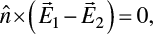
For two linear and isotropic media, Eqs. (1.2.1a)–(1.2.1d) lead to electromagnetic boundary conditions at the medium interface as follows:
 (1.2.3a)
 (1.2.3b)
 (1.2.3c)
 (1.2.3d)
where  is a unit vector normal to the interface of the two media. Using Eqs. (1.2.1a) and (1.2.1b), we can obtain the following relation:


 (1.2.4)
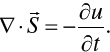
where we implicitly assume that the medium is homogeneous, isotropic, and linear. Based on Eq. (1.2.4), we can introduce the Poynting vector  specifying electromagnetic energy flow and the electromagnetic energy density (u) as follows:
 (1.2.5)
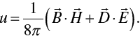 (1.2.6)
Thus, Eq. (1.2.4) is an expression of electromagnetic energy conservation in the form
 ((1.2.7))
To consider the transport of electromagnetic energy, let us compute ∇ × Eq. (1.2.1b), which leads to
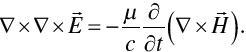 (1.2.8)
Expanding the left-hand side of Eq. (1.2.8) and substituting (1.2.1a) into the right-hand side of Eq. (1.2.8), we obtain
 (1.2.9)
Because of  based on Eqs. (1.2.1c) and (1.2.2a), we obtain the wave equation for the electric field as follows:
 (1.2.10)
Similarly, we can derive the wave equation for the magnetic field:
 (1.2.11)
The quantity  is referred to as the refractive index. We denote it by m.
Equations (1.2.10) and (1.2.11) together govern the propagation of an electromagnetic wave. In these two equations,  is the phase speed of the wave in the medium. In this book, we only consider time harmonic waves and assume that the temporal dependence is in the form of
 , where
 and
 is the angular frequency. This choice is consistent with the counterpart in many texts such as Born and Wolf (Reference Born and Wolf1999), Bohren and Huffman (Reference Bohren and Huffman1983), and Mishchenko et al. (Reference Mishchenko, Travis and Lacis2002). With the temporal-dependence factor
 , the imaginary part of the complex index of refraction in the frequency domain is non-negative (i.e., the quantity can be zero or a positive number) for an absorbing medium. Alternatively, as an equally valid approach, the temporal-dependence factor can be specified as
 , such as in van de Hulst (Reference van de Hulst1957) and Liou (Reference Liou2002). The latter choice leads to a non-positive (i.e., the quantity can be zero or a negative number) imaginary part of the complex index of refraction in the frequency domain for an absorbing medium. Whether we select
 or
 , the final analysis gives the same measurable quantities. However, a specific choice of the temporal factor must be used in a consistent form in downstream derivations and formulae as pointed out by Bohren and Huffman (Reference Bohren and Huffman1983) and Mishchenko et al. (Reference Mishchenko, Travis and Lacis2002). Throughout this text, we will use the temporal-dependence factor
 to specify a time harmonic wave; therefore, the electric and magnetic fields can be expressed in the form
 (1.2.12)
where  indicates the position vector. The light-scattering processes involved in this book are constrained to the case of elastic scattering; that is, the electromagnetic wave frequency is not changed in the scattering process.
With the expression in Eq. (1.2.12), we can simplify Maxwell’s equations in their time-independent form as follows:
 (1.2.13a)
 (1.2.13b)
 (1.2.13c)
 (1.2.13d)
where 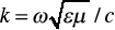 is referred to as the modified wavenumber in a medium with the index of refraction
 .
For a time-harmonic wave in optical analysis, we normally consider the average of a measurable quantity within a temporal duration T much longer than  . Thus, the time-averaged Poynting vector is given by

 (1.2.14)
where the asterisk indicates complex conjugation. Note that because 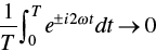 if
 , Eq. (1.2.14) can be simplified in the form

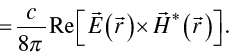 (1.2.15)
Thus, we can now define the complex Poynting vector, where only the real part is physically meaningful, as:
 (1.2.16)
Similarly, the harmonic electromagnetic energy density is given by
 (1.2.17)
Furthermore, for a homogeneous (i.e., the planes of constant phase are parallel to the planes of constant amplitude) plane electromagnetic wave propagating along a direction indicated by a unit vector  with the electric field in the form of
 (1.2.18a)
 (1.2.18b)
where  is the complex amplitude of the wave, and
 is a unit vector pointing along vector
 , that is,
 .
If we select  as the time-dependent factor for a plane electromagnetic wave in an absorbing (with a nonzero effective electric conductivity
 ) nonferromagnetic, medium (
 ), the complex refractive index in the frequency domain is given by
 , or
 , and
 . In this case, the time-averaged Poynting vector is given by

 (1.2.19)
It is clear from the above equation Eq. (1.2.19) that the magnitude of the Poynting vector decreases with the electromagnetic wave propagation if  is nonzero, that is,
 .
1.2.2 Stokes Parameters
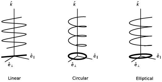
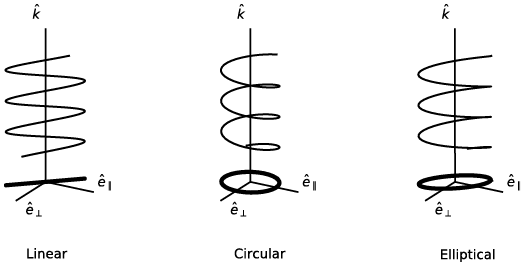
An electromagnetic wave is a vector wave; that is, its electric and magnetic fields must be specified in terms of both their magnitudes and directions. The vibration configuration of the electric field vector is referred to as the polarization state of the wave. Perrin (Reference Perrin1942) presented a thorough review of the polarization state. The polarization state is referred to as linear, circular, or elliptical if the projection of the end point of the electric vector on a plane transverse to the propagation direction traces out a straight line, a circle, or an ellipse, respectively, as schematically illustrated in Figure 1.6. In the case of circular or elliptical polarization, the polarization state is said to be right-handed or left-handed for an observer facing the incoming light (i.e., the observer looks toward the light source) if the end point of the electric field vector describes a helix in a clockwise or anticlockwise form, respectively (Born and Wolf, Reference Born and Wolf1999). The opposite convention has also been used in the literature by defining the observation to be looking along the light propagation direction (van de Hulst, Reference van de Hulst1957; Hovenier et al., Reference Hovenier, van der Mee and Domke2004). In this text, the convention of right-/left-handed polarization follows the traditional definition described in Born and Wolf (Reference Born and Wolf1999) by looking toward the light source, which is also consistent with Bohren and Huffman (Reference Bohren and Huffman1983) and Mishchenko et al. (Reference Mishchenko, Travis and Lacis2002).
Illustration of the polarization states of linearly, circularly, and elliptically polarized waves. The waves propagate along the direction specified by unit vector 
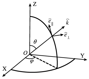
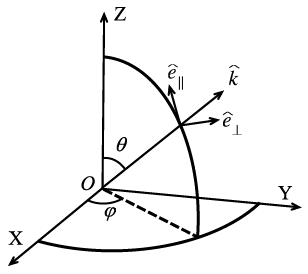
Most optical instruments do not directly measure the electric and magnetic fields, mainly because the fields are highly oscillatory complex quantities. To overcome this difficulty, four real-valued optically measurable quantities referred to as the Stokes parameters, introduced originally by Stokes (Reference Stokes1862), can be used. To define the Stokes parameters, let us consider a plane electromagnetic wave in a vacuum as follows:
 (1.2.20)
where  and
 are two orthogonal unit vectors, and unit vector
 points along the propagation direction of the wave, as illustrated in Figure 1.7. The quantities
 and
 are the projections of the electric field vector onto the directions specified by
 and
 , respectively. Note that
 and
 can be complex quantities and are often referred to as the parallel and perpendicular electric field components with respect to the meridional plane specified in terms of zenith angle
 and azimuthal angle
 , as shown in Figure 1.7. With such a decomposition of the electric field vector associated with a wave in a nonabsorptive medium with relative permittivity
 and relative permeability , the Stokes parameters can be defined in the form
 (1.2.21a)
 (1.2.21b)
 (1.2.21c)
 (1.2.21d)
where the asterisk indicates complex conjugation and  . The Stokes parameters have the dimension of irradiance, namely power per unit area. Note that the convention of the Stokes parameters in Eqs. (1.2.21a)–(1.2.21d) is consistent with many texts such as van de Hulst (Reference van de Hulst1957), Bohren and Huffman (Reference Bohren and Huffman1983), and Mishchenko et al. (Reference Mishchenko, Travis and Lacis2002). However, Liou (Reference Liou2002) introduces a negative sign to component V. Moreover, the sign difference of the V component may cause confusion in the definition of left-handed and right-handed circular polarization. Note that the I, Q, and U components are not affected by the choice of the time dependence, but the sign of the V component depends on both the sign choice in Eq. (1.2.21d) and the representation of harmonic waves in the form of either
 or
 . Because the Stokes parameters are usually considered in a relative sense, the constant factor
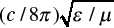 in Eqs. (1.2.21a)–(1.2.21d) can be omitted in many cases without affecting the relevant analysis. Thus, following Bohren and Huffman (Reference Bohren and Huffman1983) and Mishchenko et al. (Reference Mishchenko, Travis and Lacis2002), we will not include this constant factor in the following discussions.
Reference plane for defining the Stokes parameters.
For a monochromatic harmonic wave, it will be shown later that the four Stokes parameters are not independent, and they satisfy the following relation:
 (1.2.22)
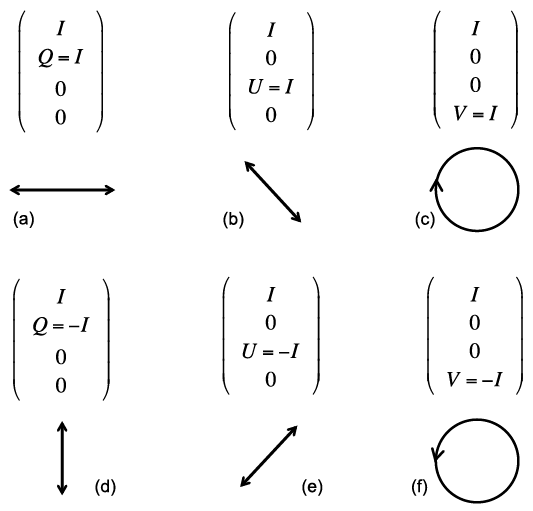
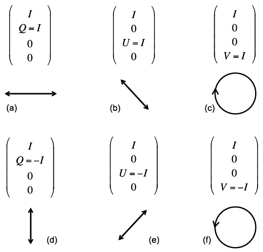
The Stokes parameters fully specify the characteristics of a light beam; in particular, any optical analysis is not capable of distinguishing two light beams that have the same Stokes parameters (Chandrasekhar, Reference Chandrasekhar1960). Among the Stokes parameters, the quantity I specifies the intensity of light, the quantities U and V specify the linear polarization, and V specifies circular polarization, as illustrated by Figure 1.8. Thus, it is natural to introduce the degree of polarization (DoP):
 (1.2.23)
the degree of circular polarization (DoCP) as
 (1.2.24)
and the degree of linear polarization (DoLP) as
 (1.2.25)
In the case of  , DoLP is usually defined as follows (Hovenier et al., Reference Hovenier, van der Mee and Domke2004):
 (1.2.26)
Polarization configurations for linearly polarized light (panels a, b, d, and e) and circularly polarized light (panels c and f). Note that the light propagation direction points out of the paper (the observer looks toward the light source). Panel (c) illustrates right circular polarization and panel (f) illustrates left circular polarization.
Let us assume the phases of the parallel and perpendicular electric field components to be  and
 , and the real amplitudes of the two electric field components to be
 and
 . Then, we can rewrite Eq. (1.2.20) in the form
 (1.2.27)
With the representation of the electric field in Eq. (1.2.27), along with omitting the constant factor 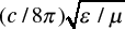 , the Stokes parameters can be given in the form
 (1.2.28a)
 (1.2.28b)
 (1.2.28c)
 (1.2.28d)
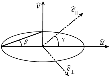
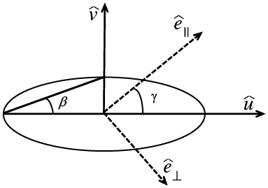
The most general polarization state is elliptical polarization, where the projection of the end point of the electric vector on a plane transverse to the propagation direction traces out an ellipse. If we define two unit vectors  and
 to be along the semi-major and semi-minor axes of the ellipse as shown in Figure 1.9, the real part of the electric vector can be expressed in the form
 (1.2.29)
where  denotes a constant phase difference. Because the intensity of the light beam is independent of the coordinate system employed to specify the polarization state, the following relation must hold:
 (1.2.30)
Geometric configuration of elliptical polarization. Note that this diagram depicts quantities in the  plane. Angles
 and
 are defined in the text.
Because of the relation 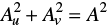 , we introduce an angle
 such that
 (1.2.31a)
 (1.2.31b)
The sign of  is defined positive for right-handed polarization and negative for left-handed polarization. The geometric meaning of angle is illustrated in Figure 1.9, that is,
 indicates the ellipticity of the ellipse, namely,

To project the real part of the electric vector in Eq. (1.2.29) onto the two directions specified by  and
 , we obtain
 (1.2.32a)
 (1.2.32b)
The above equations Eqs. (1.2.32a) and (1.2.32b) can be further expanded and rearranged as follows:
 (1.2.33a)
 (1.2.33b)
Because  and
 are linearly independent, Eqs. (1.2.33a) and (1.2.33b) lead to
 (1.2.34a)
 (1.2.34b)
 (1.2.34c)
 (1.2.34d)
Based on Eqs. (1.2.34a)–(1.2.34d), the Stokes parameters can be written with respect to the amplitude and the orientation angle as depicted in Figure 1.9. On squaring and adding Eqs. (1.2.34a) and (1.2.34b), we obtain the intensity along the  direction
 (1.2.35)
Similarly, Eqs. (1.2.34c) and (1.2.34d) lead to
 (1.2.36)
Adding the product of Eqs. (1.2.34a) and (1.2.34c) to that of (1.2.34b) and (1.2.34d), we obtain
 (1.2.37)
where  . Subtracting the product of Eqs. (1.2.34b) and (1.2.34c) from that of (1.2.34a) and (1.2.34d) yields
 (1.2.38)
Taking the quotient of Eqs. (1.2.34b) and (1.2.34a), we have
 (1.2.39)
Similarly, the quotient of Eqs. (1.2.34d) and (1.2.34c) gives
 (1.2.40)
therefore
 (1.2.41)
Note that sines and cosines of the angles ,  , and can be simultaneously switched in Eqs. (1.2.32)–(1.2.34), to represent the geometry of the polarization. In that case, Eqs. (1.2.35)–(1.2.38) and (1.2.41) will not be changed, but Eqs. (1.2.39) and (1.2.40) will be given by
 (1.2.42)
 (1.2.43)
With Eqs. (1.2.28), (1.2.35)–(1.2.38), it is straightforward to show that the Stokes parameters in geometric notation can be expressed in the form (van de Hulst, Reference van de Hulst1957)
 ((1.2.44a))
 (1.2.44b)
 (1.2.44c)
 (1.2.44d)
The four Stokes parameters associated with the electric field specified by Eq. (1.2.27) are not completely independent, as they depend on only three quantities, namely, A, , and in Eqs. (1.2.44a)–(1.2.44d). Based on Eq. (1.2.44), it is straightforward to show that  . From Eq. (1.2.44), the orientation of the polarization ellipse and the ellipticity can be specified by
 (1.2.45a)
 (1.2.45b)
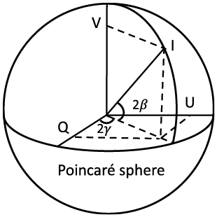
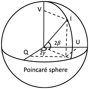
Furthermore, it is obvious that the relations in Eqs. (1.2.44a)–(1.2.44d) imply that Q, U, and V can be used as spherical coordinates. Thus, the Stokes parameters can be represented using a spherical coordinate system, the so-called Poincaré sphere as illustrated in Figure 1.10, following Born and Wolf (Reference Born and Wolf1999).
Representation of the Stokes parameters on the Poincaré sphere.
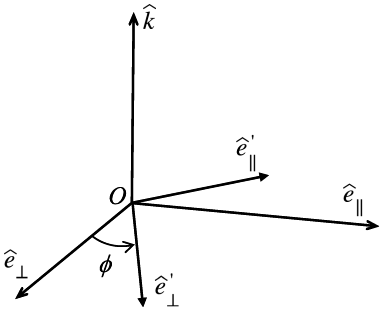
The Stokes parameters are specified with respect to a specific reference plane. As shown in Figure 1.11, the decomposition of the electric field vector associated with the rotation of a coordinate system is
 (1.2.46a)
 (1.2.46b)
where  is defined as the clockwise rotation angle of the
 axis to the
 axis for an observer looking along the propagation direction specified by unit vector
 . The transformation represented by Eqs. (1.2.46a) and (1.2.46b) can be expressed in a matrix form as
 (1.2.47)
Rotation of a reference coordinate system for the electric field decomposition.
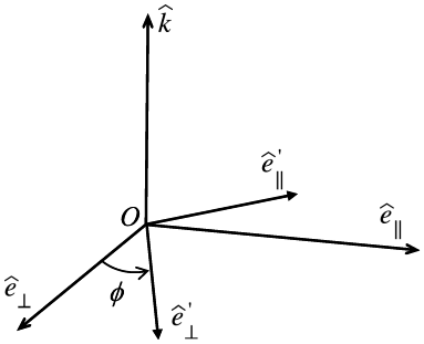
As a result of the field transform in Eqs. (1.2.46a) and (1.2.46b), the rotational transform for the Stokes parameters is given by
 (1.2.48)
It can be shown that, with the rotational transform given by Eq. (1.2.48),  ,
 , and
 are invariant. In addition, the degree of polarization defined by Eq. (1.2.23), the degree of circular polarization defined by Eq. (1.2.24), the degree of linear polarization defined by Eq. (1.2.25), and the ellipticity specified in terms of
 (see Figure 1.9) are also invariant.
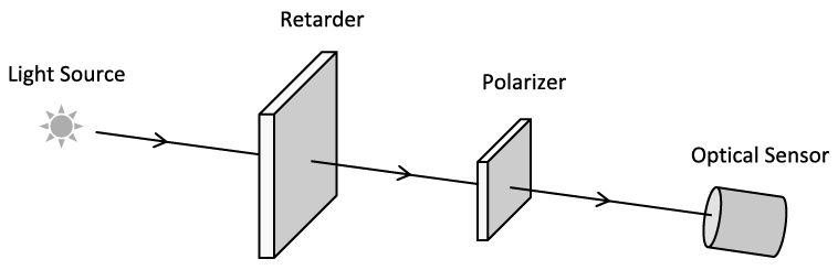
Later we recapture the experimental methodology described by Chandrasekhar (Reference Chandrasekhar1960) and Bohren and Huffman (Reference Bohren and Huffman1983) for measuring the Stokes parameters. Specifically, Figure 1.12 schematically illustrates an experimental setup for measuring the Stokes parameters. Specifically, a wave retarder introduces a certain amount of retardation in the phase of one of the two components of the electric field decomposed with respect to the  and
 directions. In the following discussion, we assume the phase difference between
 and
 components of the electric field vector to be
 . The polarizer constrains the measurement of the electric field vector component vibrating in only one direction and deviating from the
 axis by an angle , which is called the direction of the transmission axis of the linear polarizer.
Schematic diagram illustrating the measurement of the Stokes parameters.
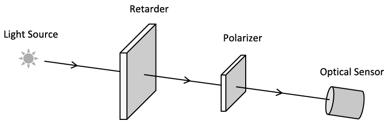
Following Chandrasekhar (Reference Chandrasekhar1960), the measured radiance can be expressed as a function of angles and in the form of
 (1.2.49)
where  and
 . Using Eq. (1.2.49), let us consider the following four polarization cases:
Case 1: Natural light, that is, unpolarized with 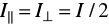 ,
 , and
 . Thus, we have
 (1.2.50)
Case 2: Horizontal and vertical polarization configurations without a retarder for a polarized incident beam ( and two measurements with
 and
 ). In this scenario, we have
 (1.2.51a)
 (1.2.51b)
Thus, the first two Stokes parameters can be given by
 (1.2.52a)
 (1.2.52b)
Case 3: +45° and −45° polarization configurations without a compensator (for a polarized incident beam),  and two measurements with
 and
 . In this scenario, we have
 ((1.2.53a))
 (1.2.53b)
From Eq. (1.2.53), we obtain
 (1.2.54)
Case 4: Measurement of circular polarization using +45° and −45° polarization configurations with a quarter-wave plate ( and two measurements with
 and
 ). In this scenario, we have
 (1.2.55a)
 (1.2.55b)
From Eq. (1.2.55), we obtain
 (1.2.56)
For an arbitrarily polarized light beam, the measurements associated with Eqs. (1.2.51), (1.2.52), (1.2.54), and (1.2.56) can fully quantify the Stokes parameters of the light beam.
1.2.3 Amplitude Scattering Matrix and the Optical Theorem
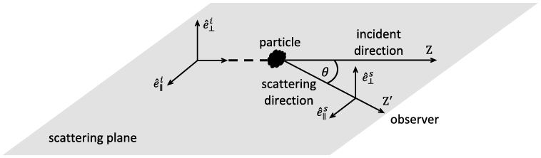
Figure 1.13 illustrates the general configuration of the scattering of light by a particle. The observer is far away from the scattering particle, and thus, the observed scattered field is in the far-field zone (i.e., the distance between the observer and the particle is much larger than the wavelength of the incident light). The direction pointing from the particle to the observer is referred to as the scattering direction, and the scattering angle is the angle between the incident and scattering directions. The plane containing the incident and scattering directions is called the scattering plane. If the scattering particle has axial symmetry around the z-axis, the scattering properties are independent of the rotation of the scattering plane around the symmetric axis of the particle, that is, the z-axis in the present case. In the most general case, the scattering properties depend on the rotation of the scattering plane around the z-axis.
Schematic diagram illustrating the configuration of the scattering of light by a particle, where superscripts i and s refer to the incident and scattering directions, respectively.
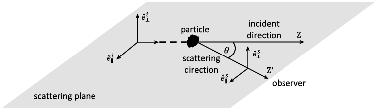
As shown in Figure 1.13, both incident and scattered electric vectors can be decomposed into parallel and perpendicular components with respect to the scattering plane. With the decomposition, we have the following relation
 (1.2.57)
where k is referred to as the modified wavenumber in a vacuum, given by  where λ is the wavelength. r (>> λ) is the distance between the observer and the scattering particle, and
 are the elements of the amplitude scattering matrix. Here we use the popular notation introduced originally by van de Hulst (Reference van de Hulst1957) for the amplitude scattering matrix, namely,
 (1.2.58)
The amplitude scattering matrix contains essentially all the optical information about the elastic scattering and absorption properties of the scattering particle. In particular, the amplitude scattering matrix elements in the forward direction are directly related to the extinction cross section of the particle. To illustrate this feature, we consider the far-field region near the forward direction 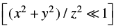 , where the following approximation is valid:
 (1.2.59)
Thus, the scattered field in the forward direction can be given by
 (1.2.60)
The first Stokes parameter associated with the total electromagnetic field (the incident field plus the scattered field) can be given in the form
 (1.2.61)
where superscript t indicates the total irradiance. The earlier irradiance can be decomposed into two components:
 (1.2.62)
where  is the incident irradiance and
 is associated with the extinction process. These components are given by
 (1.2.63)

 (1.2.64)
The extinction cross section of the particle can be calculated via
 (1.2.65)
From Eq. (1.2.65) and the double Fresnel integral given by
 (1.2.66)
it is straightforward to formulate the extinction cross section as follows:
 (1.2.67)
It is evident from Eq. (1.2.67) that the extinction cross section is determined by the amplitude scattering matrix in the forward direction and by the polarization state of the incident electromagnetic radiation, although scattering occurs in all directions and the extinction cross section is the sum of the scattering and absorption cross sections. If the incident radiation is unpolarized  , the extinction cross section given by Eq. (1.2.67) reduces to
 (1.2.68)
If  and are the same [hereafter, indicated by
 ], such as in the case of the scattering of light by a sphere, Eq. (1.2.68) reduces to the form of the optical theorem given in most texts:
 (1.2.69)
Note that the approximation  assumed in Eq. (1.2.59) can be avoided by using an alternate approach based on the asymptotic behavior (Jones and Kline, Reference Jones and Kline1958) of integral
 (Bohren and Huffman, Reference Bohren and Huffman1983).
It is apparent that the extinction cross section of a particle may depend on the polarization state of the incident light. This optical phenomenon is analogous to the dichroism observed in conjunction with anisotropic materials (Mishchenko et al., Reference Mishchenko, Travis and Lacis2002; Mishchenko, Reference Mishchenko2008). Shefer and Popov (Reference Shefer and Popov2010) investigated the elements of the extinction matrix based on physical optics and reported that the off-diagonal elements differ from the first element by an order of magnitude.
To quantify the effect of the polarization state on the extinction cross section, we introduce a factor:
 (1.2.70)
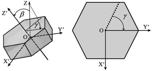
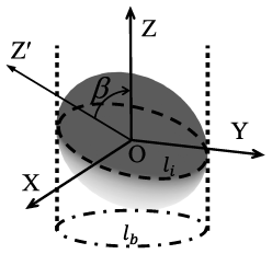
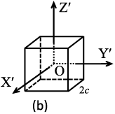
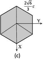
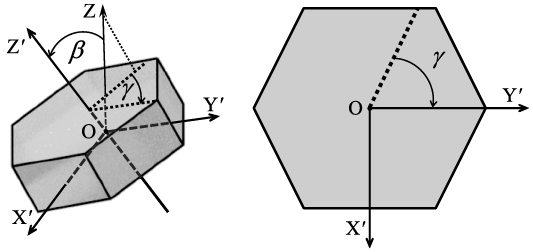
To illustrate the dependence of the earlier factor on the polarization state of the incident light, let us consider the scattering of polarized light by a hexagonal plate. As shown in Figure 1.14a, OX′Y′Z′ is a particle coordinate system fixed to the particle, and OZ is the z-axis of the incident-light coordinate system, pointing along the incident direction. The orientation of the particle system relative to the incident-light system can be specified in terms of three Euler angles , , and . Figure 1.14 illustrates the definition of angles and . Angle (not shown in Figure 1.14) indicates the rotation of the particle around the Z-axis. The extinction cross section of the particle depends on and but independent of .
(a) Illustration of Euler angles and in a three-dimensional plot. OX′Y′Z′ is the particle coordinate system. OXYZ is the incident-light coordinate system (only the Z axis is shown). The incident direction is along OZ. is the angle between OZ and OZ′. is the angle between the projection of OZ on the OX′Y′ plane and OY′. (b) A top view of the particle along OZ′. The dashed line is the projection of OZ on the OX′Y′ plane. The definition of is shown.
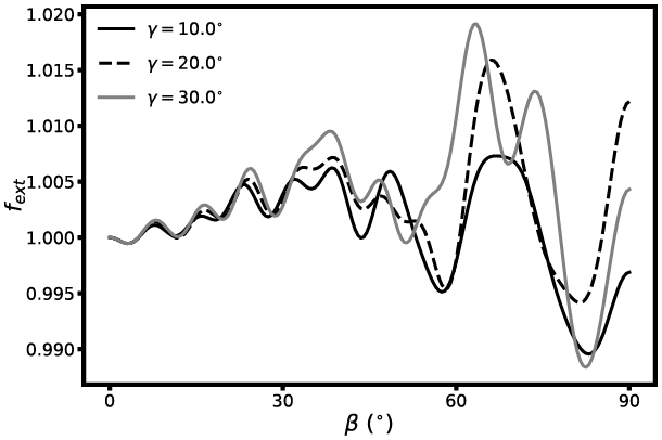
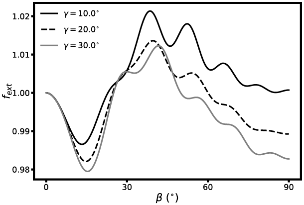
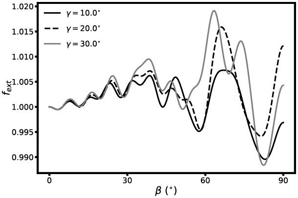
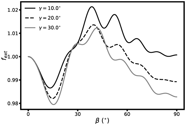
Figures 1.15 and 1.16 show  as a function of the orientation of a hexagonal column and plate for the incident light with a Stokes vector of (1,1,0,0) based on the IITM (Johnson, Reference Johnson1988; Bi and Yang, Reference Bi and Yang2014a). The aspect ratio of the hexagonal column is 1.5 and the counterpart of the hexagonal plate is 0.5. The refractive index is 1.3 + i0.0, the size parameter defined in terms of the height of the hexagonal column and the thickness of the hexagonal plate is 30, and angle indicates the tilting of the symmetry axis of the particle from the zenith. As demonstrated in Figures 1.15 and 1.16,
 can be either larger or less than unity, depending on the particle orientation as well as particle shape (i.e., the particle aspect ratio in the present case).
Effect of the polarization state and the orientation of a hexagonal column with a refractive index of m = 1.3 + i0.0 on the extinction of light. Three orientations are considered and specified by angles equal to 10°, 20°, and 30°.
The same as Figure 1.15, but for a hexagonal plate.
In summary, the extinction cross section depends on particle orientation and the polarization state of the incident light. Specifically, the extinction cross section for a linearly polarized radiation beam can be larger or smaller than that for an unpolarized radiation beam, depending on the orientation of the scattering particle with respect to the incident direction. Furthermore, it should be pointed out that the complete extinction matrix rather than the scalar extinction cross section is required for describing the transfer of polarized light (Mishchenko et al., Reference Mishchenko, Travis and Lacis2006) in a scattering medium consisting of oriented particles.
1.2.4 Scattering Phase Matrix
In conjunction with the transformation of the incident electric field to the scattered electric field in Eq. (1.2.57), the corresponding transformation for the Stokes parameters is in the form
 (1.2.71)
where superscripts s and i indicate the scattered and incident light, respectively. F is a 4 × 4 matrix in the form
 ((1.2.72))
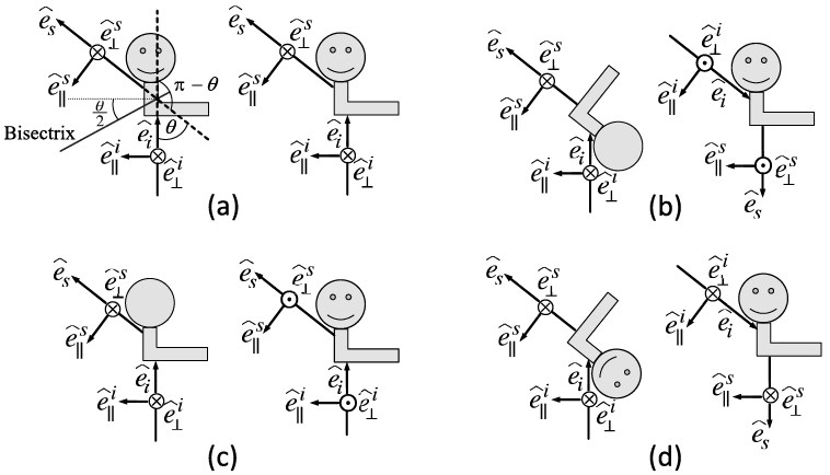
The F matrix elements are not independent in some scenarios. The relationships of the elements are discussed in many studies (Perrin, Reference Perrin1942; van de Hulst, Reference van de Hulst1957; Takano and Jayaweera, Reference Takano and Jayaweera1985; Hu et al., Reference Hu1987; Hovenier and van de Mee, Reference Hovenier and van der Mee1996; Hovenier and Mackowski, Reference Hovenier and Mackowski1998). Figure 1.17 illustrates the incident-scattering configurations for an arbitrarily shaped particle at its reciprocal and mirror positions and can be used to explain the relationships of the F matrix elements. In the laboratory coordinate system, the incident and scattering directions are fixed. The position of the particle varies in Figure 1.17(b)–(d). In the particle coordinate system, the particle’s position is fixed and the incident and scattering directions vary. In reference to the configuration depicted in Figure 1.17a, the line that is confined on the scattering plane and bisects the angle (π − ) between the incident and scattering directions is referred to as the bisectrix, and the plane through the bisectrix and normal to the scattering plane is referred to as the bisectrix plane (van de Hulst, Reference van de Hulst1957). Figure 1.17b depicts the reciprocal configurations. In particular, the original particle position is rotated 180° about the bisectrix to result in the reciprocal position. The reader is referred to Hovenier et al. (Reference Hovenier, van der Mee and Domke2004) for a clear explanation of the reciprocity principle in the context of light scattering by an individual particle. The configurations shown in Figure 1.17c and 1.17d correspond to the mirror configurations of those in Figure 1.17a and 1.17b, respectively. Note that the configurations illustrated in Figure 1.17(a) and the left panels of Figure 1.17(b)–(d) are, in principle, the same as van de Hulst’s illustrations presented with respect to the incident-light system, while the illustrations in the right panels of Figure 1.17(b)–(d) are presented with respect to the particle coordinate system in the same form as Sun et al. (Reference Sun2020).
Illustrations of the incident and scattering directions in laboratory and particle coordinate systems. The illustration on the left of each panel is in principle the same as that in van de Hulst (Reference van de Hulst1957) and shows the incident  and scattering
 directions and associated polarization directions, in reference to the laboratory coordinate system. The illustration on the right of each panel is in reference to the particle coordinate system. The scattering plane formed by the incident and scattering directions is coplanar with the paper. (a) An arbitrarily shaped particle in its original position. The incident-scattering configurations are identical in laboratory and particle coordinate systems.
 is the scattering angle. A bisectrix bisects the angle π − ; (b) the particle is at the reciprocal position (van de Hulst, Reference van de Hulst1957) with respect to (a), and is obtained by rotating it 180° about the bisectrix; (c) the particle is at the mirror position with respect to (a); (d) the particle is at the mirror position with respect to (b). In (c) and (d), the mirror is the scattering plane.
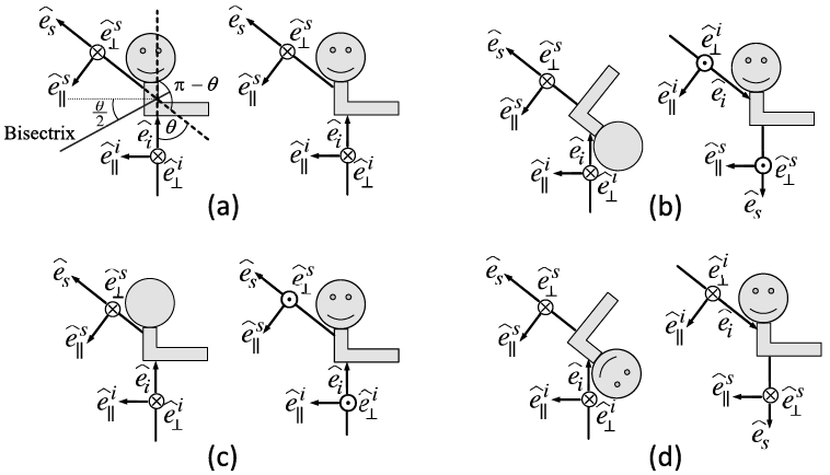
When the amplitude scattering matrix and the phase matrix corresponding to configuration 1.17a are given by Eqs. (1.2.58) and (1.2.72), respectively, the amplitude scattering and phase matrices corresponding to Figures 1.17b, 1.17c, and 1.17d are given by
 (1.2.73)
 (1.2.74)
 (1.2.75)
 (1.2.76)
 (1.2.77)
 ((1.2.78))
For many applications, such as in atmospheric remote sensing implementations and plane-parallel radiative transfer simulations, we need to consider a scattering particle system that can be reasonably assumed to be randomly oriented with an equal number of mirror-image positions with respect to both the scattering plane and the reciprocal position plane. This of course implies that there are equal numbers of particles in positions (a)–(d) in Figure 1.17. In this text, we assume this random orientation condition for the particles unless specifically stated. Furthermore, we assume that the scattering by an ensemble of particles or a particle system is incoherent, implying that the scattering phase matrix of the particle system is given by the sum of those of the individual particles in the particle ensemble. Under such assumptions, the mean matrix F of the particle system can be simplified based on Eqs. (1.2.72) and (1.2.76) as

 (1.2.79)
where
 (1.2.80a)
 (1.2.80b)
 (1.2.80c)
Takano and Jayaweera (Reference Takano and Jayaweera1985), Hu et al. (Reference Hu1987), and Hovenier and Mackowski (Reference Hovenier and Mackowski1998) discussed the symmetry relations in the forward and backward directions for light scattering by nonspherical particles. Special attention is called for a particle with a plane of symmetry under the random orientation condition. In this case, the nonzero elements of the F matrix in the forward direction reduce to
 (1.2.81a)
 (1.2.81b)
 (1.2.81c)
If the particle is rotationally symmetric, the following relation holds in the 0° forward scattering direction (Hovenier and Mackowski, Reference Hovenier and Mackowski1998):
 (1.2.82)
For a particle under the random orientation condition, the nonzero elements of the F matrix in the backward direction reduce to (Takano and Jayaweera, Reference Takano and Jayaweera1985; Hovenier and Mackowski, Reference Hovenier and Mackowski1998)
 (1.2.83a)
 (1.2.83b)
 (1.2.83c)
If the particle has a plane of symmetry, the following relation holds in the 180° backward scattering direction:
 (1.2.84)
In practice, the relations in Eqs. (1.2.72)–(1.2.77) can largely simplify the numerical computation or they can be used to validate numerical results. Furthermore, the F matrix in Eq. (1.2.79) can be expressed in a normalized form as follows:
 (1.2.85)
where  is the scattering cross section given by
 (1.2.86)
It can be shown that  (usually, called the phase function) is normalized in the form:
 (1.2.87)
The matrix P in Eq. (1.2.85) is referred to as the normalized scattering phase matrix. In the case of the scattering of light by a sphere, we have  ,
 , and
 . Since
 for a sphere, the deviation of the ratio
 from unity is an indicator of the degree of nonsphericity (Bohren and Huffman, Reference Bohren and Huffman1983; Mishchenko et al., Reference Mishchenko, Travis and Lacis2006).
For practical applications, the scattering phase matrix elements can be expanded in terms of the generalized spherical function. In this way, a large look-up table for tabulated phase matrix element data can be avoided. In particular, following Mishchenko et al. (Reference Mishchenko, Travis and Lacis2006), we have
 (1.2.88a)
 (1.2.88b)
 (1.2.88c)
 (1.2.88d)
 (1.2.88e)
 (1.2.88f)
where  ,
 ,
 ,
 ,
 , and
 are the expansion coefficients.
 are the generalized spherical functions that are complex functions given by the Wigner d-functions. The reader is referred to Appendix F of Mishchenko et al. (Reference Mishchenko, Travis and Lacis2006) for detailed discussions of the generalized spherical functions and the Wigner d-functions.
In many practical applications where computational feasibility and efficiency are critical, we do not need the detailed angular variation of the phase function, such as in the radiative transfer models involved in climate models due to consideration of computational feasibility and efficiency. Instead, we introduce a parameter called the asymmetry factor g to quantify the overall degree of the deviation of the scattered light from the incident direction, which is given by
 (1.2.89a)
If the phase function is independent of the azimuthal angle of the scattering plane, Eq. (1.2.89a) is simplified to the following form:
 (1.2.89b)
An analytical phase function specified in terms of the asymmetry factor, known as the Henyey–Greenstein (H-G) phase function (Henyey and Greenstein, Reference Henyey and Greenstein1941), has been widely used in radiative transfer simulation, particularly for irradiance computation, and is given by
 (1.2.90)
It is worth noting that the (H-G) phase function can be analytically expanded in terms of the Legendre polynomials in the form:
 (1.2.91)
where  is the nth-order Legendre polynomials. The feature of the H-G phase function shown in Eq. (1.2.91) is convenient for the truncation of the phase function in multiple scattering (i.e., radiative transfer) simulation (e.g., Wiscombe, Reference Wiscombe1977), particularly for the two-stream radiative transfer scheme (Meador and Weaver, Reference Meador and Weaver1980) that has been extensively used for radiative flux calculations in climate models.
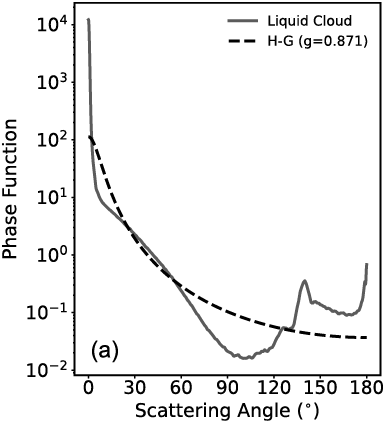
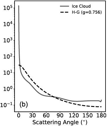
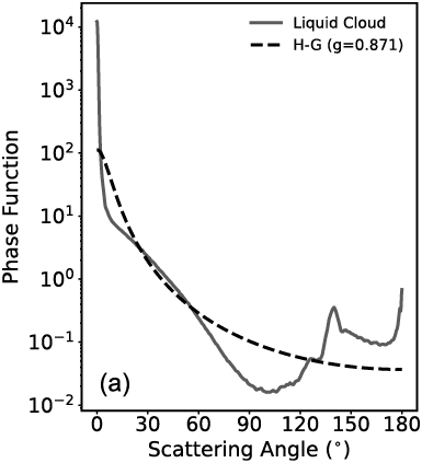
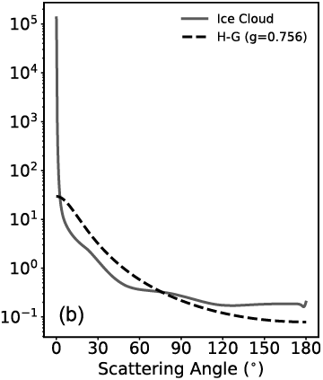
However, the H-G phase function can be quite different from a phase function with the same asymmetry factor. For example, Figure 1.18 shows the phase functions of a water cloud and an ice cloud in comparison with their corresponding Henyey–Greenstein phase function approximations. The water and ice cloud phase functions in Figure 1.18 are taken from those used in the operational MODIS cloud property retrievals (Platnick et al., Reference Platnick2017). For remote sensing applications, the detailed phase function is necessary for radiance simulation involved in generating look-up tables for implementing a retrieval algorithm. In this case, the H-G phase function is usually not applicable.
Comparison between rigorously computed liquid cloud and ice cloud phase functions and the corresponding Henyey–Greenstein (H-G) phase functions based on the same values of the asymmetry factor. In each plot, the H-G phase function has the same asymmetry factor as the cloud phase function.
Liquid cloud with effective radius 20 μm, and the asymmetry factor (g) is 0.871;
Ice cloud with effective radius 30 μm, and g is 0.756. The wavelength is 0.87 μm. Note that the effective radius is defined as 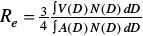 following Foot (Reference Foot1988) as a generalization of the definition of the effective radius for a polydisperse ensemble of spherical particles (Hansen and Travis, Reference Hansen and Travis1974), where D, V, and A indicate the maximum dimension, volume, and projected area of an ice crystal, respectively. N(D) indicates the particle size distribution.
1.2.5 Extinction, Scattering, and Absorption Cross Sections and Efficiencies
In Subsection 1.2.4, we have introduced the concepts of the extinction and scattering cross sections. In this section, we will give definitions of the extinction, scattering, and absorption cross sections from the perspective of energy conservation and define related efficiencies frequently used in downstream applications.
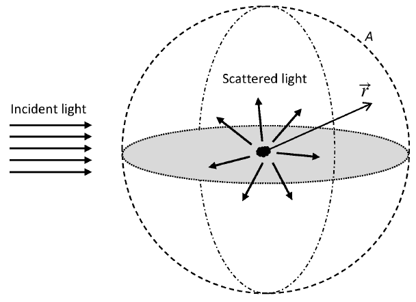
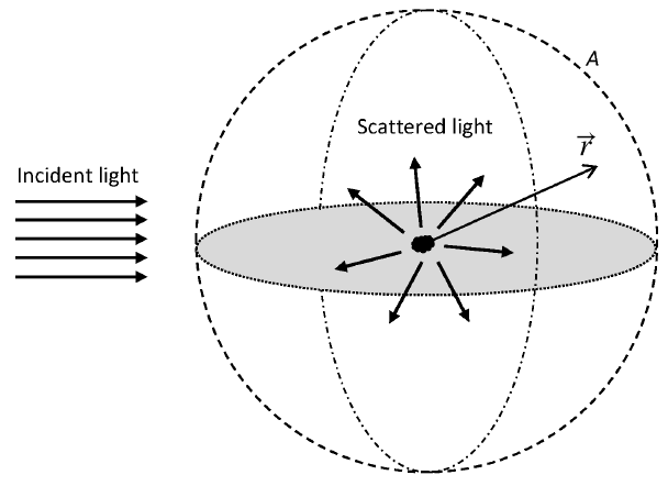
Consider a particle in a nonabsorptive medium. As shown in Figure 1.19, an incident plane wave interacts with the particle. The net rate of energy absorbed by the particle can be expressed as
 (1.2.92)
where A is the surface of an imaginary sphere surrounding the particle,  is the unit vector of
 , and subscript “a” denotes absorption. The minus sign in Eq. (1.2.92) guarantees that Wa is a non-negative value (i.e., zero or a positive value).
A schematic configuration showing a particle scattering an incident plane electromagnetic wave. An imaginary sphere (dashed curve) is plotted around the particle.  is the position vector with the particle placed at the origin.
The time-averaged Poynting vector  is given in Eq. (1.2.15). Note that, around the considered particle, the total electromagnetic field is a sum of the incident (indicated by superscript i) and scattered (indicated by superscript s) fields, given by
 (1.2.93a)
 (1.2.93b)
Substituting Eqs. (1.2.93a) and (1.2.93b) into Eq. (1.2.15), we have
 (1.2.94)
Based on Eq. (1.2.94), we can define the time-averaged Poynting vectors associated with the incident, scattered, and interaction (indicated by superscripts i, s, and int) fields,
 (1.2.95a)
 (1.2.95b)
 (1.2.95c)
Thus, we have
 (1.2.96)
Equation (1.2.95c) shows that the interaction field is generated from the incident and scattered field interaction. Substituting Eq. (1.2.96) into Eq. (1.2.92), we obtain
 ((1.2.97))
We define the net rate of energy associated with the incident, scattered, and interaction fields as
 (1.2.98a)
 (1.2.98b)
 (1.2.98c)
where the choices of signs in front of integration symbols guarantee the three quantities are non-negative. Because the incident field is a plane wave, Eq. (1.2.98a) is zero as can be proved using Gauss’s theorem. Combining Eqs. (1.2.97) and (1.2.98), we thus obtain
 (1.2.99)
which suggests the net rate of interaction field energy is the sum of the net rates of absorbed and scattered field energy. Because of energy conservation, the rate of the extinction energy is equal to the rate of the scattered and absorbed energy by the particle. Therefore, the interaction field energy is exactly the extinction energy, so we have
 (1.2.100)
Equation (1.2.95c) suggests that the extinction of electromagnetic energy is caused by the interaction between the incident and scattered fields.
Combining Eqs. (1.2.95) and (1.2.98), we have
 (1.2.101a)
 (1.2.101b)
Considering far-field scattering, the scattered electromagnetic fields are transverse to the direction vector  (i.e.,
 and
 ), and inversely proportional to the distance away from the particle (Mishchenko et al., Reference Mishchenko, Travis and Lacis2002), as suggested in Eq. (1.2.57). Thus, we have
 (1.2.102a)
 ((1.2.102b))
where r is the magnitude of  , and
 and
 are the field components only dependent on direction
 . Combining Eqs. (1.2.102) and (1.2.13b), we have
 (1.2.103)
The electric field component of the incident plane wave is expressed as
 (1.2.104)
where  is the wavevector, and its magnitude is equal to the modified wavenumber.
 is the complex amplitude. Substituting Eq. (1.2.104) into Eq. (1.2.13b), we have
 (1.2.105)
If  , the complex exponent terms in Eqs. (1.2.104)–(1.2.106) can be expressed as (Mishchenko et al., Reference Mishchenko, Travis and Lacis2002)
 (1.2.106)
so in the far-field zone, the plane electromagnetic waves in Eqs. (1.2.104)–(1.2.105) are equal to
 (1.2.107a)
 (1.2.107b)
where  is the Dirac-Delta function, and the plane wave can be seen as a superposition of incoming and outgoing spherical waves (Mishchenko et al., Reference Mishchenko, Travis and Lacis2002).
Substituting Eqs. (1.2.102)–(1.2.103), and Eq. (1.2.106) into Eq. (1.2.101), we obtain
 (1.2.108a)
 (1.2.108b)
The scattering and extinction cross sections are defined as
 (1.2.109a)
 (1.2.109b)
which suggests that during a scattering event, the scattered (extinction) energy by a particle is equal to the incident energy times the scattering (extinction) cross section. Combining Eq. (1.2.95a), Eqs. (1.2.104)–(1.2.105), and Eqs. (1.2.108)–(1.2.109), we obtain
 (1.2.110a)
 (1.2.110b)
Note that as shown in Eq. (1.2.110b), the extinction cross section is only determined by the projection of the scattered field along the incident direction, or forward scattering direction, which is consistent with the derivation in Section 1.2.3. The absorption cross section  is obtained straightforwardly,
 (1.2.111)
The extinction, scattering, and absorption cross sections of a particle can be normalized by the particle’s projected area Ap,
 (1.2.112)
where Ap is the particle’s projected area, in which case  ,
 , and
 are the dimensionless extinction, scattering, and absorption efficiencies, respectively. The efficiencies measure the ability of a particle to attenuate, scatter, and absorb light per unit projected area.
The single-scattering albedo  is an important particle optical property in radiative transfer computations, and it is defined as
 (1.2.113)
 is usually referred to as the “single-scattering co-albedo.”
Equations (1.2.109) express the scattering and extinction cross sections in terms of the scattered field. The scattering and extinction cross sections are particle optical properties, and can be expressed in terms of the amplitude scattering matrix, or scattering phase matrix elements. Combining Eqs. (1.2.57), (1.2.21), (1.2.79) and (1.2.80), Eqs. (1.2.110a) and (1.2.110b) can be written as
 (1.2.114a)
 (1.2.114b)
If the incident light is unpolarized, Eq. (1.2.114a) is consistent with Eq. (1.2.86). Equation (1.2.114b) is consistent with Eq. (1.2.67) for all incident polarization states.
1.3 Chirality and Mirror Symmetry
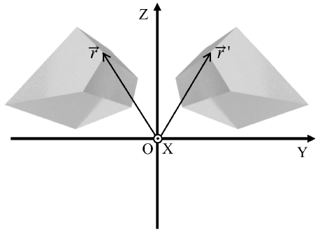
Many particles in the atmosphere and oceans that are of interest for light scattering and radiative transfer computations have an intriguing property referred to as chirality. Chirality is closely related to the concept of mirror symmetry. A particle with a fixed orientation has chirality if its mirror counterpart cannot coincide with the particle at its original orientation only through rotation operations (Kevin, Reference Kelvin1894). A good example is that the mirror image of your right hand is your left hand and no rotation can bring them to coincidence! According to this definition, a particle with a plane of symmetry or center of symmetry must be achiral. However, a particle with neither a plane of symmetry nor a center of symmetry may also be achiral (Petitjean, Reference Petitjean2020).
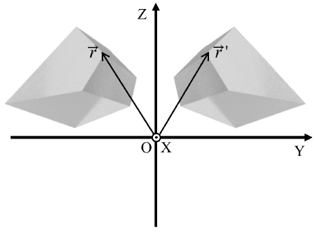
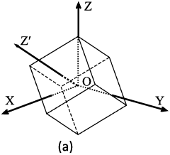
Figure 1.20 shows an example of a chiral particle and its mirror counterpart. The particle is an irregular hexahedron. We assume that the plane of mirror symmetry is the XOZ plane in the laboratory coordinate system. A point  on the original particle has coordinate in the laboratory coordinate system as
 . On the mirror particle,
 is mirrored as
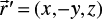 . With rotation operations on the mirror particle, not all the points on the mirror particle
 can coincide with the corresponding points
 on the original particle.
An irregular hexahedron and its mirror counterpart in a coordinate system OXYZ.  and
 are two symmetric points on the two particles.
The chirality of a particle is reflected in the single-scattering properties of the particle. The random orientation-averaged normalized scattering phase matrix of a particle (denoted by  ) is
 (1.3.1)
which is equivalent to the averaged scattering phase matrix of a collection of particles (denoted by  ) where the particle shapes are identical and the particles are randomly oriented.
 has ten independent matrix elements. Consider another collection of particles
 , where each particle is a mirror particle with respect to a particle in
 . The plane of mirror symmetry is arbitrary. The averaged scattering phase matrix of
 is thus expressed as
 (1.3.2)
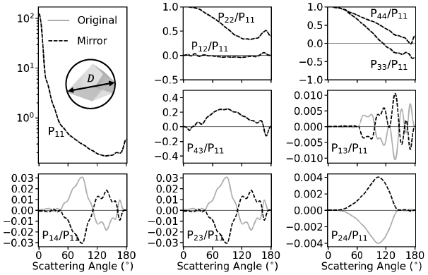
which is equal to the random orientation-averaged scattering phase matrix of the mirror particle of particle A. The upper-left four elements and lower-right four elements in  and
 are identical. The other eight elements in
 and
 have opposite signs. Furthermore, the single-scattering albedo and extinction efficiency of a particle and its mirror particle are identical, which can be straightforwardly shown using their definitions.
In the forward scattering direction, which is along the incident direction, the Stokes vector of incident field after interacting with the scattering particle is (Mishchenko et al., Reference Mishchenko, Travis and Lacis2002)
 ((1.3.3))
where  is the incident Stokes vector,
 is the incident Stokes vector after interacting with a particle, A is the area of a detector perpendicular to the incident direction, and K is the extinction matrix,
 (1.3.4)
where the matrix elements are derived from the amplitude scattering matrix in the forward scattering direction,
 (1.3.5a)
 (1.3.5b)
 (1.3.5c)
 (1.3.5d)
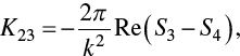 (1.3.5e)
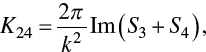 (1.3.5f)
 (1.3.5g)
Note that the diagonal elements of K are identical, but the off-diagonal elements are generally nonzero for a particle with fixed orientations, which results in the dichroism phenomenon. The incident light after interacting with scattering particles not only becomes weaker in intensity but also may have different polarization states.
According to the reciprocity of the scattering process, the extinction matrix of a randomly oriented chiral particle is expressed as
 (1.3.6)
and the extinction matrix of a mirror particle is
 (1.3.7)
Note that the nondiagonal elements  and
 are nonzero in
 and
 , and have opposite signs in
 and
 . This suggests that the random-orientation averaged extinction matrix of achiral particle only has one independent element
 , which is equal to the extinction cross section.
Figure 1.21 shows the ten normalized scattering phase matrix elements of the irregular hexahedron in Figure 1.20 and its mirror particle. The matrix elements  ,
 ,
 , and
 of the original and mirror particles are nonzero and have opposite signs. For a collection of randomly oriented chiral particles, if we assume that any particle has a corresponding mirror particle in the collection, the averaged normalized scattering phase matrix elements
 ,
 ,
 , and
 will be zero. In addition, the averaged extinction matrix elements
 and
 will be zero and the extinction matrix is the product of the extinction cross section and an identity matrix.
Normalized scattering phase matrix elements of the irregular hexahedron (Original) in Figure 1.20 and its mirror particle (Mirror), computed by the IITM. The particle has a size parameter in terms of maximum dimension (D) of 50. The refractive index is 1.53 + i0.003.
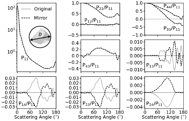
Many radiative transfer and remote sensing applications involving scattering particles such as clouds and aerosols assume that the particles are randomly oriented and contain an approximately equal number of mirror particles. As a result, the averaged scattering phase matrix only has six independent elements, and the averaged extinction matrix can be reduced to a diagonal form with the same value, namely the extinction cross section. The mirror symmetric relations involving the scattering phase matrix (Hovenier et al., Reference Hovenier, van der Mee and Domke2004) can be applied to substantially simplify radiative transfer computations. However, particles in nature are generally irregular and may not contain an equal number of mirror particles. As an example, we consider an ensemble of 20 irregular hexahedra (Saito et al., Reference Saito2021) to mimic dust aerosol single-scattering properties. The particle shapes are shown in Figure 1.22.
Shapes of 20 irregular hexahedra.
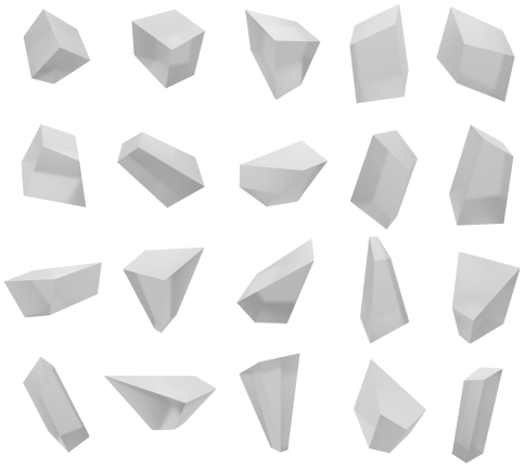
The normalized scattering phase matrix elements of the 20 irregular hexahedra in Figure 1.22 and their ensemble-averaged counterparts are shown in Figure 1.23. The corresponding nonzero extinction matrix elements are shown in Figure 1.24. Because the 20 shapes are all chiral particles, the phase matrix elements  ,
 ,
 , and
 are nonzero, and the nondiagonal extinction matrix elements
 and
 are nonzero. The ensemble-averaged scattering phase matrix can approximate the averaged scattering phase matrix of a collection of randomly oriented irregular particles with different shapes. Figures 1.23 and 1.24 show that the ensemble-averaged
 ,
 ,
 ,
 ,
 and
 are nonzero. This suggests that the assumption of randomly oriented particles with an equal number of mirror particles may not be consistent with the situation in a collection of particles with different irregular shapes and random orientations. Nevertheless, the
 ,
 ,
 ,
 ,
 and values are much smaller than other nonzero matrix elements. The errors attributed to neglecting the four phase matrix elements and two extinction matrix elements can be trivial in radiative transfer simulations and remote sensing applications.
Normalized scattering phase matrix elements of the 20 irregular hexahedra (Elements) in Fig. 1.22 and its ensemble-averaged counterpart (Ensemble), computed by the IITM. The particles have a maximum dimension (D) of 5 μm. The wavelength of the incident light is 0.865 μm. The refractive index is 1.54 + i0.0006.
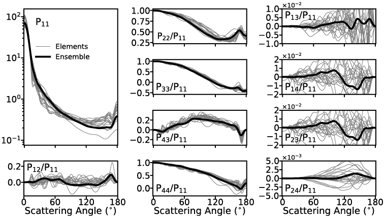
Extinction efficiency (a), and extinction matrix elements  (b) and
 (c) of the 20 irregular hexahedra (Elements) in Figure 1.22 and its ensemble-averaged counterpart (Ensemble), computed by the IITM and PGOM. The maximum dimension ranges from 0.01 to 500 μm. The wavelength of the incident light is 0.865 μm. The refractive index is 1.54 + i0.0006.
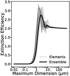
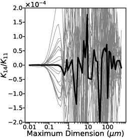
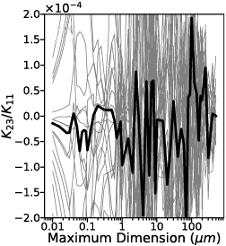
1.4 Snell’s Law, the Law of Reflection, and Fresnel Equations
Snell’s law, the law of reflection, and Fresnel equations describe the refraction and reflection phenomena of a plane electromagnetic wave propagating onto an interface, which is the boundary between two semi-infinite media with different dielectric properties. Snell’s law and the law of reflection determine the propagation directions of refracted and reflected waves. The kinematic properties of the wave, including wave intensity, phase, and polarization state, change upon reflection and refraction and are quantified by Fresnel equations. Snell’s law, the law of reflection, and Fresnel equations are introduced in many texts on electromagnetics, optics, and light scattering (e.g., Jackson, Reference Jackson1975; Born and Wolf, Reference Born and Wolf1999; Liou, Reference Liou2002). When using the ray-tracing technique based on the principles of geometric optics, one treats the electromagnetic fields as localized rays whose width must be larger than the wavelength of consideration but yet small compared to the size of the particle. The variations of the localized wave properties during ray tracing are regulated by Snell’s law, the law of reflection, and Fresnel equations. In this section, we introduce the derivation of Snell’s law, the law of reflection, and Fresnel equations from electromagnetic boundary conditions and emphasize their applications in the use of geometric optics ray tracing techniques. The media discussed in this section are nonabsorptive (i.e., the indices of refraction of the two media are real numbers), and only homogeneous electromagnetic plane waves are considered here. The cases involving absorptive media and inhomogeneous plane waves are discussed separately in Chapter 2.
1.4.1 Snell’s Law and the Law of Reflection
Snell’s law is also known as the law of refraction or the Snell–Descartes law. For consistency and conciseness, we use “Snell’s law” throughout the book.
The standard expression of Snell’s law is as follows:
 (1.4.1)
and the law of reflection is
 (1.4.2)
where superscripts “i,” “t,” and “r” represent incidence, refraction/transmission, and reflection, respectively,  and
 are the refractive indices of the two media, and
 ,
 , and
 are the angles between the normal direction of the medium interface and the propagation directions of the incident, refracted, and reflected waves, respectively. Figure 1.25 schematically depicts the definitions of these angles.
Schematic of the directions of incidence, reflection, and refraction. The electric vectors perpendicular and parallel to the incident plane are also shown. The electric vectors perpendicular to the incident plane are pointing outward from the paper.
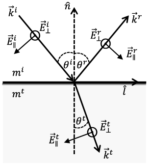
Snell’s law and the law of reflection can be derived from the electromagnetic boundary conditions. Consider the electric components of incident, reflected, and refracted plane electromagnetic waves,
 (1.4.3a)
 (1.4.3b)
 (1.4.3c)
where the time harmonic term is omitted. At the interface of the two media (the plane in Figure 1.25 containing the vectors  ,
 ,
 and
 ), according to the boundary condition Eq. (1.2.3c), we have
 (1.4.4)
To guarantee that Eq. (1.4.4) is satisfied for arbitrary  parallel to the interface, the phases of the three waves must be equal. As a result, we have
 (1.4.5)
Vector  is equal to
 , since
 is parallel to the interface, so Eq. (1.4.5) can be written as
 (1.4.6)
Because  is arbitrary, Eq. (1.4.6) is equivalent to
 (1.4.7)
Note that the wavevectors  ,
 , and
 are expressed as
 ((1.4.8a))
 (1.4.8b)
 (1.4.8c)
where  is equal to
 , and the caret indicates unit vectors. For nonferromagnetic media
 combining Eqs. (1.4.7)–(1.4.8) gives
 (1.4.9)
With the index of refraction defined in the form
 (1.4.10)
it is straightforward to prove that Eq. (1.4.9) leads to Eqs. (1.4.1)–(1.4.2).
1.4.2 Fresnel Equations
The Fresnel equations are derived from the electromagnetic boundary conditions for nonferromagnetic media 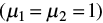 that are expressed as follows:
 (1.4.11a)
 (1.4.11b)
 (1.4.11c)
 (1.4.11d)
where the constitutive relations have been incorporated, and the two media do not contain any free charge or current.
As discussed in Section 1.2.2, the plane electromagnetic field can be written as a combination of two orthogonal components,
 (1.4.12a)
 (1.4.12b)
where the phase terms are omitted. Here  is a unit vector parallel to the incident plane formed by
 and
 in Figure 1.25, and
 is a unit vector perpendicular to the incident plane.
 and
 satisfy
 . According to Maxwell’s equations, the electric and magnetic components of a plane wave are orthogonal, and we have
 (1.4.13)
At the interface of the two media, according to the boundary conditions Eqs. (1.4.11a)–(1.4.11d), we have
 (1.4.14a)
 (1.4.14b)
 (1.4.14c)
 (1.4.14d)
Combining Eqs. (1.4.12a), (1.4.14), and (1.4.15), the components that are parallel and perpendicular to the incident plane are decoupled as
 (1.4.15a)
 (1.4.15b)
 (1.4.15c)
 (1.4.15d)
The reflection and transmission coefficients of the Fresnel equations are defined as
 (1.4.16a)
 (1.4.16b)
 (1.4.16c)
 (1.4.16d)
Combining Eqs. (1.4.15)–(1.4.16) and Eqs. (1.4.7)–(1.4.10), the Fresnel equations are expressed as
 (1.4.17a)
 ((1.4.17b))
 (1.4.17c)
 (1.4.17d)
The Fresnel equations are functions of the incident angle and refractive indices of the two media. According to the definitions of Fresnel equations, Eqs. (1.4.16a)–(1.4.16c) (also referred to as the reflection and transmission coefficients) relate the field amplitude of reflected and refracted electromagnetic fields to the incident field. Here we only give the Fresnel equations for the electric field. The counterparts of magnetic fields can be obtained with a similar approach. Because in geometric optics ray tracing, the localized electromagnetic waves inside and outside the scatterer are assumed to be plane waves, we only need to trace the electric field component, and therefore only the Fresnel equations for the electric fields are needed.
In the case of the refraction from an optically denser medium into an optically thinner medium (i.e.,  is larger than
 ), total reflection occurs if the incident angle is larger than the critical angle and the square root involved in Eqs. (1.4.17a)–(1.4.17d) is not a real quantity. This special case will be discussed in more detail in Section 1.4.3.
The reflectance (R) and transmission (T) relate the reflected and refracted power to the incident power and are computed from the Fresnel equations as
 (1.4.18a)
 (1.4.18b)
where the factor  in Eq. (1.4.18b) accounts for the change of the beam cross section during refraction to ensure energy conservation.
1.4.3 Total Internal Reflection and Brewster’s Angle
Based on the expression of Snell’s law, Eq. (1.4.1),  is equal to 90° under the following condition if
 :
 (1.4.19)
where  is the total internal reflection (TIR) angle (also known as the critical angle). If
 , Snell’s law would suggest that
 be larger than 1, meaning that the refraction angle is a complex number. Let us examine the Fresnel equations to determine what happens in this situation. If
 , the reflection coefficients Eqs. (1.4.17a)–(1.4.17b) are equal to unity, and so does the reflectance, which implies that all incident energy is reflected back to the medium where the incident light is specified. Although the transmission coefficients Eqs. (1.4.17c)–(1.4.17d) are nonzero, the transmission Eq. (1.4.18b) is zero. If
 , the reflection and transmission coefficients are complex numbers. It can be proved that the magnitudes of the reflection coefficient and the reflectance are equal to unity. Due to energy conservation, we must have
 (1.4.20)
Therefore, the transmission must be zero. Because the magnitude of the transmission coefficient is nonzero,  in Eq. (1.4.18b) must be zero. If
 is larger than one,
 is a pure imaginary number:
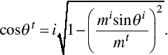 (1.4.21)
Thus,  in Eq. (1.4.18b) should be replaced with the real part of
 , which is zero when
 .
When  , the transmission coefficients are nonzero, so there is still an electromagnetic field transmitting through the medium interface. Referring to Eq. (1.2.16), the Poynting vector of the transmitted electromagnetic field is
 (1.4.22)
The component perpendicular to the interface is expressed as
 (1.4.23)
Referring to Eqs. (1.4.21), Eq. (1.4.23) is a pure imaginary number. Thus, the real part of Eq. (1.4.23) or the time-averaged Poynting vector component along  is zero. This suggests that energy does not flow through the interface when TIR occurs.
The reflection coefficient of the field component parallel to the incident plane Eq. (1.4.17b) is zero when the angle between the reflected and refracted components is 90°, which gives:
 (1.4.24)
where  is known as Brewster’s angle (Jackson, Reference Jackson1975). If the electromagnetic field is incident at Brewster’s angle, only the field component perpendicular to the incident plane is reflected. The reflected field is completely polarized, and the corresponding refracted field is partly polarized. It should be noted, however, that Étienne-Louis Malus in 1808 had already discovered the fact that many dielectrics could completely polarize light at certain angles of incidence depending on the substance (Kahr and Claborn, Reference Kahr and Claborn2008).
1.5 Fraunhofer Diffraction
Diffraction denotes various optical phenomena involving electromagnetic fields interacting with obstacles or particles. Diffraction may indicate that an incident electromagnetic wave interacts with a particle, and the resulting total field (incident + induced) amplitude and propagation directions are distinctly different from the incident field. The induced field is dependent on particle morphology and optical properties. This definition of diffraction is interchangeable with “scattering” (van de Hulst, Reference van de Hulst1957, p. 24). This book focuses mainly on the scattering of light by particles much larger than the wavelength. The incident light can be approximated as localized rays, which can exist independently and propagate rectilinearly. Here, diffraction is defined as deviation from rectilinear propagation.
In the conventional geometric optics method for solving the light-scattering problem, the scattered field is approximated as the sum of the diffracted field and the reflected and refracted fields. The diffracted field is induced by the blocking of the incident light, causing an incomplete wavefront, whereas the reflected and refracted fields are induced by the incident field impinging onto the particle. The contribution of reflection and refraction is computed with Snell’s law and Fresnel equations described in Section 1.4.3. The diffraction contribution is usually computed with Fraunhofer diffraction formulas, which will be introduced in this section.
In the current context, Fraunhofer diffraction is equivalent to the so-called far-field diffraction, where the observation location is assumed to be sufficiently far from the scatterer at a distance much larger than the incident wavelength. For many light-scattering problems, only the far-field-based single-scattering properties of a scatterer are concerned. Fraunhofer diffraction formulas are the far-field approximations of more rigorous Kirchhoff diffraction formulas. This section starts with Kirchhoff diffraction formulas to derive Fraunhofer diffraction formulas and also introduces Babinet’s principle, which is used to simplify diffraction computations in certain circumstances.
1.5.1 Scalar and Vector Kirchhoff Diffraction Formulas
The scalar Kirchhoff integral formula was first derived by Gustav Kirchhoff to more rigorously explain the Huygens–Fresnel theory. In the Huygens–Fresnel theory, the wavefront of a propagating plane wave is composed of an infinite number of wavelets. Each wavelet is a source of concentric secondary wavelets. The superposition of the spherical waves forms a plane envelope, which is the next plane wavefront. If a part of the plane wavefront is blocked by an obstacle, the incomplete wavefront will superpose to form the diffracted field. The formula of the Huygens–Fresnel theory was derived from a phenomenological description of the diffraction phenomenon. In contrast, the Kirchhoff integral formula was derived from Green’s second identity and the Helmholtz equation. The Kirchhoff integral formula was shown to be consistent with the formula of the Huygens–Fresnel theory.
Green’s second identity is expressed as (Arfken and Weber, Reference Arfken and Weber1995)
 (1.5.1)
where V is a volume, S is the surface enclosing V, and  is the normal vector of S pointing outward from V. u and v are defined in V and are second-order differentiable. The Helmholtz equation can be obtained by substituting the electric field in time harmonic form, Eq. (1.2.12), into the wave equation, Eq. (1.2.10),
 (1.5.2)
The scalar counterpart of Eq. (1.5.2) is
 (1.5.3)
The Green’s function g of the scalar field in Eq. (1.5.3) satisfies
 (1.5.4)
In Eq. (1.5.1), let u be  , and let v be g. Then, we obtain
 (1.5.5)
In a diffraction and scattering problem, the explicit form of g in a 3D space is
 (1.5.6)
which describes an outgoing radiating field and satisfies the Sommerfeld radiation condition (Jackson, Reference Jackson1975). Combining Eqs. (1.5.5)–(1.5.6), we have
 (1.5.7)
Now consider a finite area Sa. As shown in Figure 1.26, the closed surface S is composed of Sa and  .
Illustration of a diffraction problem with an incident plane wave. Sa is the area of an opening on an infinite diffraction screen. Sb is the area of part of the screen on the unilluminated side.  is the area of a surface in an infinite distance. Sa, Sb, and
 form a closed surface.
 is on the closed surface.
 is the point where the diffraction integral is evaluated.
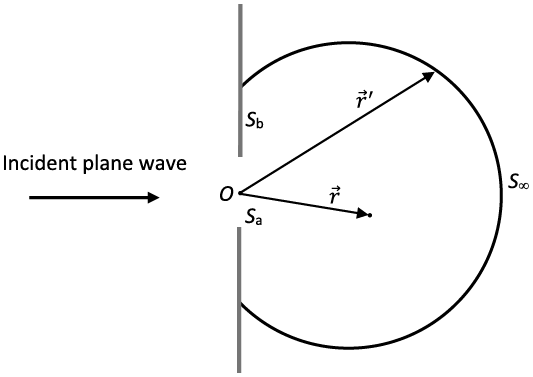
The surface integral in Eq. (1.5.7) has two separate parts on Sa and  .
 is infinitely far from the origin. As
 , the surface integral on
 vanishes since
 is proportional to the inverse of
 as an outgoing radiating field. Thus, Eq. (1.5.7) is simplified to
 (1.5.8)
where  is induced by the field on the surface Sa. Eq. (1.5.8) is the scalar Kirchhoff integral. In practice, we usually make approximations that
 and
 are equal to the counterparts of the incident field on the openings of the Sa, and vanish elsewhere on the Sa. Although the approximations are not mathematically consistent (Jackson, Reference Jackson1975), they are sufficiently accurate enough for light-scattering calculations in the far-field region in the case of a large particle.
The scalar Kirchhoff integral can only compute diffraction by a scalar field. In light-scattering calculations, to account for polarization induced by the scatterer, we need to consider a vector field to compute the diffraction of a vector field using the following vector Kirchhoff integral. According to Eq. (1.2.8), the electric vector satisfies
 (1.5.9)
for a time-harmonic field in a source-free medium. Here we rely on the dyadic Green’s function (Tai, Reference Tai1994) to derive the vector Kirchhoff integral. The dyadic Green’s function of the electric field satisfies (Tai, Reference Tai1994; Mishchenko et al., Reference Mishchenko, Travis and Lacis2002)
 (1.5.10)
where  is the dyadic Green’s function, and
 is the unit dyadic. The explicit form of
 can be derived from the relation between the electric vector and Hertz potential (Stratton, Reference Stratton1941),
 (1.5.11)
Now consider Green’s second identity involving a vector and a dyadic,
 (1.5.12)
which is derived from Green’s second identity for two vectors (Stratton, Reference Stratton1941). Let  be
 and
 be
 . Substituting Eqs. (1.5.9)–(1.5.10) into Eq. (1.5.12), we have
 (1.5.13)
If the volume V contains the point  where
 is singular, the left-hand side of Eq. (1.5.13) is equal to
 so we obtain a vector version of Eq. (1.5.5). To simplify Eq. (1.5.13), we first exclude the point
 by dividing V into two regions V1 and V2. V1 is an infinitesimal region containing the point
 and with closed surface S1. V2 is the region between S1 and S, so vector calculus relations can be used to simplify Eq. (1.5.13) in V2. In regions V1 and V2, Eq. (1.5.13) is written as
 (1.5.14)
Now we focus on region V2. Substituting Eq. (1.5.11) [the definition of  ] and Eq. (1.2.13b) into Eq. (1.5.14), we obtain
 (1.5.15)
Using Gauss’s theorem, we can further simplify the third term in the square bracket of Eq. (1.5.15) in the form
 (1.5.16)
where Eq. (1.2.13a) is used to obtain the electric vector from the magnetic vector. Combining Eqs. (1.5.14)–(1.5.16), we have
 (1.5.17)
Analogous to the scalar Kirchhoff integral Eq. (1.5.8), we obtain the vector Kirchhoff integral for a finite area Sa,
 (1.5.18)
1.5.2 Babinet’s Principle
According to the Kirchhoff approximation, the electromagnetic field at the opening of a diffraction screen is equal to the incident field and vanishes elsewhere on the screen. In a light-scattering problem, the diffraction by a particle is computed by assuming that the projection of the particle along the incident direction on a plane perpendicular to the incident light is a diffraction screen. Using the Kirchhoff approximation, the field on the projection is zero, and the field on the remaining portion on the same plane of the projection is identical to the incident field. Thus, the surface integral areas in Eqs. (1.5.8) and (1.5.18) are infinite planes excluding the particle’s projection. This may make the evaluation of the surface integral very complicated. Instead, we can utilize Babinet’s principle to simplify the integration calculation.
Now consider two diffraction screens A and B as shown in Figure 1.27. The two screens do not overlap each other in space. Screen A extends into infinity on the plane and has an aperture of the same shape and size as Screen B. If screens A and B are put on the same plane, screen B can perfectly overlap the aperture of screen A. In other words, screens A and B are complementary screens to each other. The scalar diffracted fields by A and B are denoted as  and
 . According to Eq. (1.5.8), the only difference between
 and
 is the integration area. The diffracted field by A + B is
 that is the value when no screen is present. We thus have
 (1.5.19)
Because screen A + B is a plane that extends into infinity,  is identical to the incident plane wave. Equation (1.5.19) indicates that a diffraction screen and its complementary screen have the same diffraction pattern, which is referred to as Babinet’s principle. In the directions other than the incident direction,
 . In this case, we have
 , implying the phase of the diffraction waves associated with the two screens differ by π. And the corresponding diffraction intensities are the same, that is,
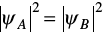 . Along the incident direction, we have
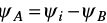 , where
 is the incident field.
Illustration of complementary screens.
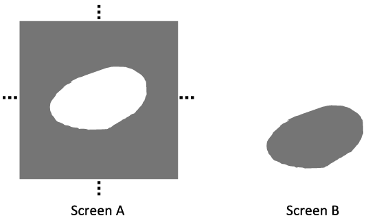
Babinet’s principle is defined for a two-dimensional (2D) diffraction screen. It has been shown that Babinet’s principle can approximate diffraction by a 3D object with acceptable accuracy (Sun et al., Reference Sun, Yang, Kattawar and Mishchenko2017a). The earlier discussion is for scalar diffraction. Babinet’s principle for vector field diffraction can be obtained analogously (e.g., Jackson, Reference Jackson1975). Because Babinet’s principle for vector field diffraction is rarely used in PGOMs to simulate light scattering, we will not discuss it here.
1.5.3 Fraunhofer Diffraction Formulas
For a light-scattering problem, we are interested in the far-field scattering properties of the scattering particle, that is, in the case where the distance between the particle and observer is much larger than the particle size and incident wavelength. The diffraction contribution is the far-field diffraction, also known as Fraunhofer diffraction. The Fraunhofer diffraction formulas can be derived by applying the far-field approximation to the Kirchhoff diffraction formulas, as described later.
The distance between the particle and observer is represented by  in Eq. (1.5.6). If
 , in which
 and
 , we have
 (1.5.20)
where  . Substituting the approximate Eq. (1.5.20) into Eq. (1.5.6) and in the denominator only keeping the r term, and also in the exponent term of Eq. (1.5.6), if
 , then we keep the
 term since the phase is more sensitive to location variation. Thus, the Green’s function in free space Eq. (1.5.6) can be approximated as
 (1.5.21)
The scalar Kirchhoff integral Eq. (1.5.8) becomes
 (1.5.22)
If  is a plane wave, then it can be written as
 where
 is a constant. Now using the Kirchhoff approximation, we can further simplify Eq. (1.5.22) as
 (1.5.23)
which is the scalar Fraunhofer diffraction formula. Alternative expressions of Fraunhofer diffraction formulas can be found in Born and Wolf (Reference Born and Wolf1999) and Jackson (Reference Jackson1975).
Similarly, we can obtain the vector Fraunhofer diffraction formula by substituting Eq. (1.5.21) into Eq. (1.5.18):
 (1.5.24)
where the transverse wave condition  is implicitly used in the derivation, because the far field is a transverse wave. Assume that the incident field is a plane wave expressed as
 (1.5.25a)
 (1.5.25b)
where  and
 are two orthogonal unit vectors and satisfy
 . Then, the far field can also be expressed as the sum of two orthogonal components,
 (1.5.26)
where  and
 satisfy
 . Substituting Eqs. (1.5.25)–(1.5.26) into Eq. (1.5.24), we obtain
 (1.5.27)
where the diffraction amplitude matrix Sd is expressed as
 (1.5.28)
Without loss of generality, we set both  and
 to be perpendicular to the diffraction/scattering plane which is formed by
 and
 . Equation (1.5.28) can then be simplified as
 (1.5.29)
Note that the diagonal elements of Sd have the same surface integral as the scalar Fraunhofer diffraction formula Eq. (1.5.23).
Using Stokes’ theorem, the surface integrals in Eqs. (1.5.23) and (1.5.29) can be written as line integrals,
 ((1.5.30))
 (1.5.31)
where la is a closed curve of Sa boundary with orientation along  according to the right-hand rule.
The line integral expressions are computationally convenient for a diffraction screen of a polygon shape. Consider a diffraction screen with N vertices 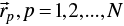 . For the line segment
 ,
 and
 in Eqs. (1.5.30)–(1.5.31) can be parameterized by
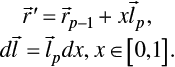 (1.5.32)
Substituting Eq. (1.5.32) into Eq. (1.5.30), the line integrals can be analytically evaluated,
 (1.5.33)
Line integrals in Eq. (1.5.31) can be evaluated in the same manner as in Eq. (1.5.33).
Combining Eqs. (1.5.29)–(1.5.33), the diffraction amplitude matrix elements are obtained as
 (1.5.34)
 ((1.5.35))
where if p =1,  .
Analogous to the definition of the F matrix element F11 in Section 1.2.4, the diffracted field intensity can be defined as
 (1.5.36)
For scalar diffraction, comparing Eqs. (1.5.23) and (1.5.29) leads to the diffracted field intensity expressed in the form  . According to Eq. (1.5.29), only when
 ,
 , and
 are on the same plane, the off-diagonal elements of the amplitude matrix are zero for all diffraction directions. This suggests the scalar diffraction formula, compared to the vector formula, may underestimate diffraction intensity.
As an example, let us consider a diffraction screen shown in Figure 1.28. The screen has a square opening, which in the xoy plane has four vertices,
 (1.5.37)
Diffraction geometry of a diffraction screen in the XOY plane with a square opening.
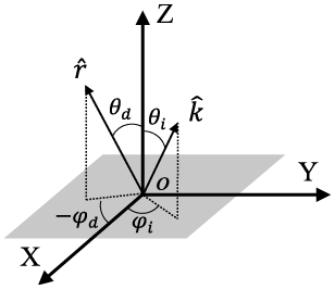
 and
 are explicitly expressed as
 (1.5.38)
 (1.5.39)
The diffraction intensity is also determined by the wavelength of the incident light and diffraction screen size in addition to the incident and diffracted directions. Equations (1.5.34)–(1.5.35) explicitly show that the diffraction amplitude matrix elements are dependent on the size-to-wavelength ratio, or the size parameter. Figure 1.29 shows angular diffraction intensities with different incident directions and diffraction azimuth angles. The size parameter ka is 100. Diffracted energy is mainly concentrated in the forward direction. The local minima and maxima are the results of interference. It is evident that the scalar diffraction formula underestimates the diffraction intensity if  ,
 and
 are not on the same plane. Therefore, in light-scattering computations, we should use the vector diffraction formula to account for the diffraction contribution.
Diffraction intensity of a square diffraction screen computed by vector and scalar diffraction formulas of a square screen opening shown in Figure 1.28. The size parameter ka is 100.
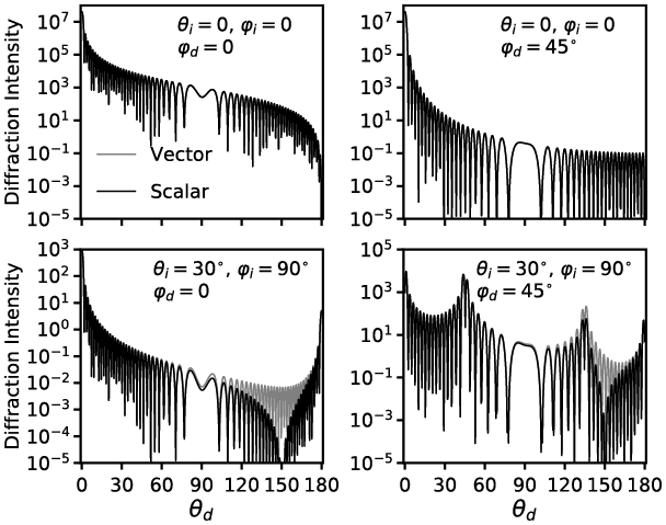
1.5.4 On the Applicability of Babinet’s Principle
In Subsection 1.5.2, we introduced Babinet’s principle. In a light-scattering problem, a part of the scattered light is attributed to Fraunhofer diffraction and can be computed using the Fraunhofer diffraction formulas derived in Subsection 1.5.3. Note that the surface integration area in Fraunhofer diffraction formulas is the area that is not blocked by the diffraction screen. In realistic numerical calculations, instead of evaluating Fraunhofer integrals on the area excluding the projection of the particle along the incident direction, we always apply Fraunhofer diffraction formulas to the projection of the particle along the incident direction. Thus, Babinet’s principle is indeed utilized here.
For a 2D object, according to Babinet’s principle, the diffraction pattern is identical to the one by its complementary diffraction screen. A particle is a 3D object, whereas its projection is on a 2D plane. Thus, a question arises: Is the diffraction by a 3D object equivalent to the diffraction of its projection along the incident direction? To answer this question, we must compare the diffraction calculation result of Babinet’s principle with the exact diffraction of a 3D particle. Previous studies, for example, Brillouin (Reference Brillouin1949), Bi et al. (Reference Bi2011), and Sun et al. (Reference Sun, Yang, Kattawar and Mishchenko2017a), discussed the applicability of Babinet’s principle to diffraction by a 3D particle. In this subsection, we use the electromagnetic surface integral equation to compute the exact diffraction of a 3D particle and compare it with Babinet’s principle both theoretically and numerically.
The electromagnetic surface integral equation is derived from Maxwell’s equations and can be seen as a generalization of the Fraunhofer diffraction formulas introduced in Subsection 1.5.3. The detailed derivation of the surface integral equation is given in Chapter 3. Here we directly use it to compute Fraunhofer diffraction by a 3D particle. The electromagnetic surface integral equation is written as
 (1.5.40)
which is similar to the Fraunhofer diffraction integral Eq. (1.5.24). The subscript “sca” denotes the scattered field. The surface integration area of Eq. (1.5.40) is the closed surface of a particle rather than a diffraction screen  , and
 is the outward normal vector of the particle surface. The expressions of Eqs. (1.5.24) and (1.5.40) differ by a minus sign, since the orientations of their normal vectors are defined in opposite directions.
With the surface integral Eq. (1.5.40), the scattered field can be assumed to be a linear superposition of the diffracted field, externally reflected field, and internally reflected field. The electric and magnetic fields in the integrand of Eq. (1.5.40) are on the exterior surface of the particle. The diffracted field is induced by the incident field. Substituting the incident electric and magnetic fields of Eq. (1.5.25) into Eq. (1.5.40), we obtain the diffracted electric field,
 ((1.5.41))
where the integration area  is the illuminated side of the particle and
 . Similar to Eq. (1.5.29), we obtain diffraction amplitude matrix elements:
 (1.5.42a)
 (1.5.42b)
where  . The diffracted field intensity is calculated by Eq. (1.5.36).
Babinet’s principle is applied to the projection of the particle along the incident direction. The particle projection is a diffraction screen and blocks the incident light. Using Babinet’s principle, the diffraction pattern by the projection is the same as its complementary screen, which has an opening identical to the projection. Thus, the Fraunhofer diffraction formulas can be applied to the projection area and take the incident field as the integrand. Note that the diffracted field by the complementary screen has the opposite sign compared to the original projection counterpart. The diffraction amplitude matrix elements using Babinet’s principle are directly derived from Eq. (1.5.29),
 (1.5.43a)
 (1.5.43b)
where  is used, and then the sign of the amplitude matrix is reversed because of Babinet’s principle. Superscript “b” denotes that Babinet’s principle is applied.
 is the projection area of the particle along the incident direction. The diffracted field intensity of the result based on Babinet’s principle result can be represented in the same manner in Eq. (1.5.36),
 (1.5.44)
It is obvious that if  is a constant vector and
 , then
 and
 . In the following, we consider the situation
 . For exact forward diffraction
 , as in Eqs. (1.5.30)–(1.5.31), the diffraction amplitude matrix elements can be written as
 ((1.5.45a))
 (1.5.45b)
 (1.5.45c)
 (1.5.45d)
where  is the closed curve of the illuminated area
 and
 is the closed curve of the projection
 . It can be straightforwardly proved that the line integrals in Eqs. (1.5.45a) and (1.5.45c) are equivalent, so that Babinet’s principle and surface integral approaches generate identical forward diffraction.
If  , the diffraction amplitude matrix elements can be written as line integrals as in Eqs. (1.5.30)–(1.5.31),
 (1.5.46a)
 (1.5.46b)
 (1.5.46c)
 (1.5.46d)
Generally,  and
 are nonzero, and the line integrals in Eqs. (1.5.46a) and (1.5.46c) are not equal if
 is not on the plane perpendicular to the incident direction. In addition,
 may not stay in the same plane in the case of a 3D particle.
We now consider diffraction by two particle shapes, spheroid and cube, and compare the diffraction calculation results by the surface integral and Babinet’s principle methods. The boundary curve of the illuminated side of a spheroid is always in one plane, but the counterpart of a cube can be in different planes depending on the cube’s orientation relative to the incident direction.
Consider a spheroid defined in the particle coordinate system in the form of
 (1.5.47)
where a and c are semi-axis lengths, and the rotationally symmetric axis is along the  direction. The orientation of the spheroid in the laboratory coordinate system can be described by Euler’s angles as illustrated in Subsection 1.2.3. The equation of an arbitrarily oriented spheroid in laboratory coordinates is given by Lock (Reference Lock1996a). Without loss of generality, we now consider a spheroid with only the Euler angle nonzero, so the line of nodes is along the Y axis. The equation of this spheroid in laboratory coordinates is
 (1.5.48)
where the constants A and B are defined for conciseness,
 (1.5.49a)
 (1.5.49b)
The incident direction is along the Z direction so the vectors involved in the diffraction calculation defined in laboratory coordinates can be explicitly written as
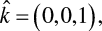 (1.5.50a)
 (1.5.50b)
 (1.5.50c)
 (1.5.50d)
An illustration of spheroid diffraction is shown in Figure 1.30. Since the formulas Eqs. (1.5.42) and (1.5.46a,b) are equivalent, we can use either of them to compute the diffraction based on an electromagnetic surface integral. Furthermore, according to Stokes’ theorem, the surface integral of a vector field on an arbitrary smooth surface enclosed by  is equal to the corresponding line integral along
 . Thus, instead of applying the surface integral Eq. (1.5.42) on the illuminated surface
 , we can simply evaluate the surface integral on the ellipse enclosed by
 , which is denoted as
 hereafter.
Illustration of diffraction by a spheroid. The rotationally symmetric axis is along  . The incident direction is along Z. The dashed ellipse denotes the boundary of the illuminated area
 and the dot-dashed ellipse denotes the boundary of projection
 .
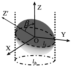
The integration area  can be described as the intersection of the spheroid and a plane. To determine the intersection plane, we consider the normal vector of the spheroid surface,
 (1.5.51a)
 (1.5.51b)
Since  is the boundary curve dividing illuminated and unilluminated surfaces, along
 the normal vector must satisfy
 . Combining Eqs. (1.5.50a) and (1.5.51), we have
 (1.5.52)
so  is on the plane with the equation
 (1.5.53)
 is an ellipse with semi-axis lengths
 and
 ,
 (1.5.54a)
 (1.5.54b)
The normal vector of  can be straightforwardly obtained from Eq. (1.5.53),
 (1.5.55)
To evaluate the integrals in Eq. (1.5.42), a point  on
 can be parameterized as
 (1.5.56)
where  and
 are unit orthogonal vectors and are perpendicular to
 .
 and t are radial and angular coordinates, respectively.
 and
 are written as
 (1.5.57a)
 (1.5.57b)
Substituting Eqs. (1.5.50), (1.5.54), (1.5.56), and (1.5.57) into the integral in Eq. (1.5.42), we have
 (1.5.58)
where  is a constant and
 is defined as
 (1.5.59)
An integral representation of the Bessel function of the first kind is
 (1.5.60)
When  , using the recurrence relation
 (1.5.61)
and comparing Eqs. (1.5.60) and (1.5.58), we have
 (1.5.62)
where 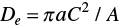 is the area of
 . Combining Eqs. (1.5.42), (1.5.50), and (1.5.62), we obtain the expressions of diffraction amplitude matrix elements by the electromagnetic surface integral method,
 (1.5.63a)
 (1.5.63b)
The expressions of diffraction amplitude matrix elements by Babinet’s principle can be derived in a similar manner. For the Babinet’s principle-based method, the integration area is the projection of the spheroid on the XY plane along the incident direction. The projection is an ellipse, and its equation can be derived by substituting Eq. (1.5.53) into Eq. (1.5.48),
 (1.5.64)
With a similar derivation procedure, we obtain the nonzero diffraction amplitude matrix elements by Babinet’s principle method,
 (1.5.65)
where  is the area of the integration area
 and
 is written as
 (1.5.66)
Comparison of diffraction intensity computed by the electromagnetic surface integral (SI) and Babinet’s principle (BP) methods for a spheroid illustrated in Figure 1.30 and related text. The spheroid has kc = 100 and ka = 50, and Euler angle = 45°.
The relative azimuth angle is 0;
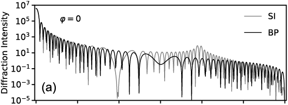
The relative azimuth angle is 45°.
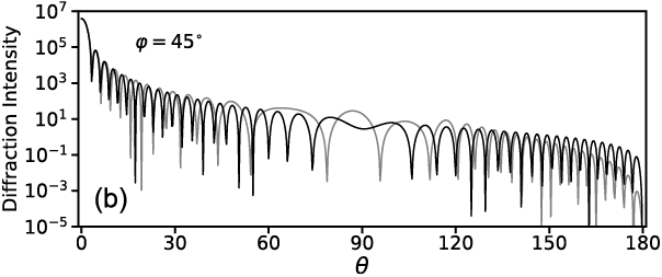
An example of numerical calculation by the electromagnetic surface integral and Babinet’s principle methods is shown in Figure 1.31. At a viewing zenith angle less than about 10°, the two methods are almost identical. At other angles, the two methods show obvious differences. For example, for the case with the relative azimuth angle equal to 0, the peak around 120° by the surface integral method is not captured by the method based on Babinet’s principle.
We then consider a cube with particle coordinates X′, Y′, and Z′ perpendicular to two faces each and passing through the faces’ geometric centers. The Euler’s angles relative to the laboratory coordinate are  . Figure 1.32 shows the cube in both the laboratory and particle coordinates. The cube has side length 2c. Its illuminated side has three identical squares, which are not on the same plane. In Figure 1.32c, the projection of the cube against the incident direction (the Z-axis direction onto the XY plane) is a regular hexagon with side length
 .
A cube with side length 2c.
Cube in laboratory coordinates;
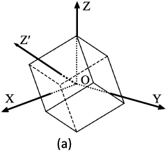
Cube in particle coordinates;
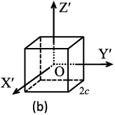
Cube’s projection along the Z direction onto the XY plane.
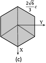
The line integral forms Eqs. (1.5.45) and (1.5.46) are more mathematically convenient for faceted particles. The illuminated side involves seven vertices,
 (1.5.67)
The three illuminated squares’ vertices are listed as follows:
 (1.5.68)
The diffraction amplitude matrix associated with one illuminated square can be calculated in the same manner as Eqs. (1.5.34) and (1.5.35). The total diffraction amplitude matrix is the sum of the three squares’ contribution,
 (1.5.69a)
 (1.5.69b)
To apply Babinet’s principle method, we consider the projection of the cube on the XY plane shown in Figure 1.32(c). The vertices of the projection are
 (1.5.70)
The diffraction amplitude matrix of the hexagon can be calculated in a similar manner as Eqs. (1.5.34) and (1.5.35), too. The numerical comparison of the electromagnetic surface integral and Babinet’s principle methods is shown in Figure 1.33. At the viewing zenith angle less than 10°, the two methods generate almost identical results. At other viewing zenith angles, they are not consistent. With a relative azimuth angle of 45°, the peaks around = 40° and 90° by the surface integral method are not captured by the Babinet’s principle based method.
Comparison of diffraction intensity computed by the electromagnetic surface integral (SI) method and Babinet’s principle (BP) for a cube illustrated in Figure 1.32 and related text. The cube has kc = 100.
The relative azimuth angle is 0;
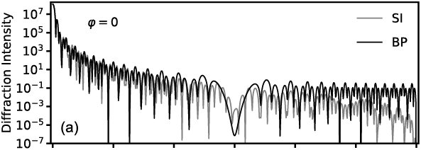
The relative azimuth angle is 45°.
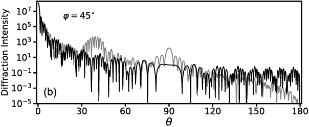
The earlier theoretical and numerical results indicate the fact that the Babinet’s principle-based computation is not equivalent to the exact diffraction calculation for which the 3D geometry of the scattering particle is fully considered. As demonstrated earlier and by Sun et al. (Reference Sun, Yang, Kattawar and Mishchenko2017a), the diffraction by a particle depends on the boundary that separates the illuminated and shadowed sides of the particle instead of the particle surface morphology. If the aforementioned separating boundary is confined in the same plane normal to the incident direction, Babinet’s principle is as accurate as the electromagnetic surface integral method, such as in the case of spheres and spheroids when the incident direction is parallel to the particle’s rotational axis. However, the majority of diffracted energy is concentrated in the forward diffraction angles, where the Babinet’s principle-based method is very accurate. Furthermore, if we consider orientation-averaged particle diffraction, the errors of the Babinet’s principle-based method can be significantly reduced. In summary, the Babinet’s principle-based method is reasonably accurate to compute diffraction by a 3D particle much larger than the wavelength of the incident light, especially when only orientation-averaged results are considered.