2 Waleffe flow

Plane Couette flow is generated by rigid parallel walls located at $y=\pm h$ moving with opposite velocities $\pm U$ in the streamwise direction. In contrast, the system we consider is driven by a sinusoidal body force to produce a laminar shear profile confined by stress-free boundary conditions:

depicted in figure 2(a). Typically, periodic boundary conditions are imposed in the lateral streamwise, $x$ , and spanwise, $z$ , directions. The flow was first used by Tollmien to illustrate the insufficiency of an inflection point for linear instability (Drazin & Reid Reference Drazin and Reid2004). Its simplicity derives from the stress-free boundary conditions, much as stress-free boundaries have led to simplicity and insight in thermal convection (Drazin & Reid Reference Drazin and Reid2004). Waleffe (Reference Waleffe1997) used the flow to illustrate the self-sustaining process and to derive a model of eight ordinary differential equations (ODEs) capturing the essence of the process. Extensions of this ODE model have been derived (Manneville Reference Manneville2004) and used to measure turbulent lifetimes (Moehlis, Faisst & Eckhardt Reference Moehlis, Faisst and Eckhardt2004; Dawes & Giles Reference Dawes and Giles2011) as well as to find unstable solutions (Moehlis, Faisst & Eckhardt Reference Moehlis, Faisst and Eckhardt2005; Beaume et al. Reference Beaume, Chini, Julien and Knobloch2015; Chantry & Kerswell Reference Chantry and Kerswell2015). However, there has been little study of fully resolved Waleffe flow itself in the context of turbulence. Schumacher & Eckhardt (Reference Schumacher and Eckhardt2001) studied the lateral growth of turbulent spots and Doering, Eckhardt & Schumacher (Reference Doering, Eckhardt and Schumacher2003) considered the bounds on energy dissipation in this system. Here, we undertake a systematic study of Waleffe flow throughout the transitional regime.

We simulate Waleffe flow with the freely available CHANNELFLOW (Gibson, Halcrow & Cvitanović Reference Gibson, Halcrow and Cvitanović2008; Gibson Reference Gibson2014) adapted to enforce stress-free boundary conditions. We employ 33 Chebyshev modes in the vertical direction, $y$ , and approximately 128 Fourier modes per ten spatial horizontal units.

Figure 2.

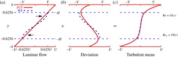
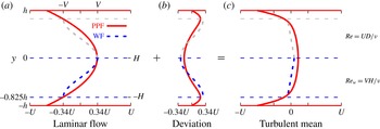
Waleffe flow (WF) seen as an approximation to the interior of plane Couette flow. Shown are streamwise velocity profiles for PCF (solid/red) and WF (dashed/blue) in the uniformly turbulent regime (PCF: $\mathit{Re}=500$ and WF: $\mathit{Re}_{w}=500$ ). Plotted are (a) laminar flow, (b) deviation of mean turbulent profile from laminar flow and (c) mean turbulent profile. The $y$ -scale of WF is non-dimensionalised using $h=1.6H$ to align its stress-free boundaries (dashed horizontals) with extrema of the PCF deviation profile in (b). WF velocities are likewise scaled by $U=1.6V$ so that both flows have the same average laminar shear in (a). Data are from simulations of 2000 advective time units for $[L_{x},L_{y},L_{z}]=[12,2,10]h$ .

We begin by comparing turbulent velocity profiles for Waleffe and plane Couette flow, and use these to establish a scaling relationship between the flows. Figure 2 shows the streamwise velocity of uniformly turbulent flow, averaged over time and the horizontal directions, decomposed into the sum of the laminar profile and the deviation from laminar. Lengths in WF have been scaled to align its stress-free boundaries with the extrema of the PCF deviation profile (figure 2 b) and velocities have been scaled to maintain the average laminar shear (figure 2 a). WF effectively captures the interior section of PCF – the section between the extrema of the deviation profile, figure 2(b), or equivalently the section excluding the boundary layers associated with no-slip walls, figure 2(c). This was first observed by Waleffe (Reference Waleffe2003) for an exact solution (exact coherent structure) shared by PCF and by another stress-free version of PCF.

The preceding paragraph implies that when treating WF as the interior of PCF, WF should be non-dimensionalised by length and velocity scales given by $H=h/1.6=0.625h$ and $V=0.625U$ . These values are not intended to be exact, since the extrema of the PCF profiles depend on $\mathit{Re}$ , although weakly over the range of interest here (from $y/h\simeq \pm 0.60$ at $\mathit{Re}=300$ to $y/h\simeq \pm 0.65$ at $\mathit{Re}=700$ ). This rescaling of $y$ is almost identical to that arrived at by Waleffe (Reference Waleffe2003) through a different line of reasoning. A value close to this one could also be obtained from the extrema of low-order polynomial approximations, like those used for modelling by Lagha & Manneville (Reference Lagha and Manneville2007a ,Reference Lagha and Manneville b ), although these $y$ values would necessarily deviate from the actual values with increasing Reynolds number. The effective Reynolds number for WF, comparable to that for PCF, is then

where $\mathit{Re}_{w}\equiv VH/{\it\nu}$ is the Reynolds number usually used for WF.

Simulating Waleffe flow in large domains, we observe robust turbulent bands emerging from uniform turbulence as the Reynolds number is decreased. Figure 1(d) shows such bands under conditions equivalent to those for PCF in figure 1(c). There is remarkably strong resemblance in the broad features of the two flows. The primary difference is that in WF the positive (red) and negative (blue) streaks are less distinct and are almost entirely separated by the turbulent-band centre, while in PCF the streaks are more sharply defined and may pass through the turbulent centre.

Figure 3.

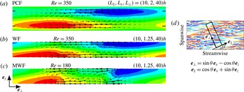
Comparison of bands in (a) plane Couette flow, (b) Waleffe flow and (c) model Waleffe flow, showing the deviation from the laminar flow in a cross-sectional plane, averaged both in $t$ and along $\boldsymbol{e}_{\Vert }$ . The turbulent region is centred at the middle of the domain. Through-plane flow is depicted by contours from negative (blue) to positive (red) and in-plane flow is depicted by arrows. Contour levels are scaled to 10 % below extrema, $\text{PCF}\in [-0.34,0.34]$ , $\text{WF}\in [-0.42,0.42]$ and $\text{MWF}\in [-0.41,0.41]$ . For visibility the $y$ -direction in all flows has been stretched by a factor of 3. Tick marks at $y=\pm 0.625h$ in panel (a) indicate the bounds of the interior region to which Waleffe flow corresponds. (d) Planar view of a minimal titled domain in relation to a larger domain.

For a quantitative study of the banded structure, we simulate the flows in domains tilted by angle ${\it\theta}$ in the streamwise–spanwise plane as illustrated in figure 3(d). Tilted domains are the minimal flow unit to capture bands (Barkley & Tuckerman Reference Barkley and Tuckerman2005) and they provide an efficient and focused method for quantitative analysis. Domains are short ( $10h{-}16h$ ) in the direction along the bands, $\boldsymbol{e}_{\Vert }$ , and long ( $40h{-}120h$ ) in the direction across the bands, $\boldsymbol{e}_{\bot }$ , i.e. along the wavevector of the pattern. We fix the angle at ${\it\theta}=24^{\circ }$ , that of the bands seen in figure 1. This angle is typical of those observed in experiments and numerical simulations of PCF in large domains (Prigent et al. Reference Prigent, Grégoire, Chaté, Dauchot and van Saarloos2002; Duguet et al. Reference Duguet, Schlatter and Henningson2010) and is that used in previous work (Barkley & Tuckerman Reference Barkley and Tuckerman2005, Reference Barkley and Tuckerman2007; Tuckerman & Barkley Reference Tuckerman and Barkley2011) on tilted domains.

In figure 3(a,b) we compare bands in Waleffe flow to those of plane Couette flow, under equivalent conditions using the rescaling (2.2) of WF. Mean flows are visualised in the $(\boldsymbol{e}_{\bot },\boldsymbol{e}_{y})$ plane, with averages taken over the $\boldsymbol{e}_{\Vert }$ direction and over 2000 advective time units. The red and blue regions indicate the flow parallel to the turbulent bands, primarily along the edges of the bands, while the arrows show circulation surrounding them. The banded structure in Waleffe flow is almost identical to that found in the interior of plane Couette flow. Waleffe (Reference Waleffe2003) made similar observations regarding exact coherent structures in no-slip and stress-free versions of plane Couette flow. The main qualitative difference between the flows is the greater separation of the regions of positive and negative band-aligned flow in WF (figure 3 b). This is a manifestation of the streak separation in figure 1(d).

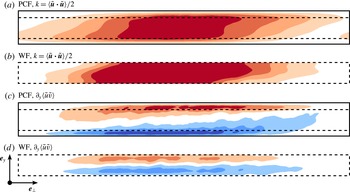
We also consider the fluctuations, $\tilde{\boldsymbol{u}}$ , about the mean flow. In figure 4 we see that in both PCF and WF the turbulent kinetic energy is largest in the interior. Beneath this we plot $\partial _{y}\langle \tilde{u} \tilde{v}\rangle$ , which dominates the turbulent force (see Barkley & Tuckerman (Reference Barkley and Tuckerman2007) for a full discussion of the force balance that prevails in turbulent–laminar banded flow). Although the turbulent force is very large in the near-wall regions of PCF, it mainly acts to counterbalance the large dissipation due to the steep gradients near the walls. In the interior of PCF, both dissipative and turbulent forces are much weaker, as is the case for the entirety of Waleffe flow.

Figure 4.

Comparison of turbulent fluctuations, $\tilde{\boldsymbol{u}}$ , in plane Couette flow and Waleffe flow for turbulent bands plotted in figure 3. (a,b) Turbulent kinetic energy, $k=\langle \tilde{\boldsymbol{u}}\boldsymbol{\cdot }\tilde{\boldsymbol{u}}\rangle /2$ for PCF (contours $[0,0.08]$ ) and WF (contours $[0,0.05]$ ) respectively, averaged as in figure 3(a–c). (c,d) Dominant turbulent force contribution in the band-aligned direction, $\partial _{y}\langle \tilde{u} \tilde{v}\rangle$ for PCF (contours $[-0.017,0.017]$ ) and WF (contours $[-0.017,0.017]$ ). Dashed lines in (a,c) show the bounds of the interior region to which Waleffe flow corresponds.

We have surveyed the intermittency in Waleffe flow as a function of Reynolds number. In the tilted domain, bands emerge from turbulence at $\mathit{Re}\approx 640$ and turbulent patches are still observed with long lifetimes ( $O(10^{3})$ time units) at $\mathit{Re}\approx 250$ , consistent with $\mathit{Re}_{w}=\mathit{Re}/2.56\approx 110$ found previously (Schumacher & Eckhardt Reference Schumacher and Eckhardt2001, figure 2). In PCF the equivalent range is $325\lesssim \mathit{Re}\lesssim 420$ (Bottin & Chaté Reference Bottin and Chaté1998; Bottin et al. Reference Bottin, Daviaud, Manneville and Dauchot1998; Tuckerman & Barkley Reference Tuckerman and Barkley2011; Shi et al. Reference Shi, Avila and Hof2013).

3 Modelling Waleffe flow

Motivated by the simplicity of Waleffe flow and its ability to capture turbulent-band formation without the boundary layers present near rigid walls, we have developed a minimal model using only leading Fourier wavenumbers in the shear direction $y$ . Our model of Waleffe flow (MWF) can be written as

where ${\it\beta}={\rm\pi}/2H$ . To further simplify, we use a poloidal–toroidal plus mean-mode representation

where ${\it\psi}$ , $f$ and $g$ match the $y$ -decomposition of $u$ and ${\it\phi}$ matches that of $v$ . Substituting (3.2) into the Navier–Stokes equations and applying Fourier orthogonality in $y$ , we derive our governing equations, which are seven partial differential equations in $(x,z,t)$ and six ODEs for the mean flows $f$ and $g$ . The original eight-ODE model, derived by Waleffe (Reference Waleffe1997) to illustrate the self-sustaining process, is contained within the system and can be recovered by reducing the number of modes in $y$ and imposing a single Fourier wavenumber in $x$ and $z$ . Our model is closely related to a series of models of WF and PCF by Manneville and co-workers (Manneville Reference Manneville2004; Lagha & Manneville Reference Lagha and Manneville2007a ,Reference Lagha and Manneville b ; Seshasayanan & Manneville Reference Seshasayanan and Manneville2015). The first three of these attempted to capture localised dynamics with only two modes in $y$ . Turbulent bands were not spontaneously formed or maintained; instead, spots grew to uniform turbulence. Most recently, and in parallel with our work, Seshasayanan & Manneville (Reference Seshasayanan and Manneville2015) showed that a model of PCF with four polynomial modes in the wall-normal direction produced oblique bands, albeit over a narrow range of $\mathit{Re}$ .

We simulate the model using a Fourier pseudospectral method in $(x,z)$ and time step using backward Euler for the linear terms and Adams–Bashforth for the nonlinear terms. The effective low resolution in $y$ results in a decreased resolution requirement in $(x,z)$ , with only four modes needed per spatial unit, compared with ${\sim}10$ for PCF and WF.

At high $\mathit{Re}$ , uniform turbulence is observed in the model (figure 1 b), displaying the usual streamwise-aligned streaks generated by rolls. Streaks in MWF, as well as in WF (not shown), typically have shorter streamwise extent than those in PCF. Reducing $\mathit{Re}$ , bands are found (figure 1 e) that are difficult to distinguish from those in fully resolved Waleffe flow (figure 1 d); this is also true for bands computed in the tilted domain (figure 3 b,c). The most notable qualitative difference between MWF and WF is the increased separation of the band-aligned flow regions and of the related circulating in-plane flow. We find bands in the model for Reynolds numbers $\mathit{Re}\in [125,230]$ , a large relative range of $\mathit{Re}$ and an approximate rescaling of $\mathit{Re}\in [250,640]$ for fully resolved Waleffe flow. The most likely reason for the shift in $\mathit{Re}$ is the lack of high-curvature modes in the wall-normal direction, i.e. small spatial scales that would be associated with higher dissipation. However, in a model for pipe flow (Willis & Kerswell Reference Willis and Kerswell2009) with few azimuthal modes, the $\mathit{Re}$ for transition increased relative to that of fully resolved flow.

Figure 5.

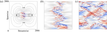
Growth of a turbulent spot in model Waleffe flow at $\mathit{Re}=160$ . The flow is initialised with a poloidal vortex and subsequent evolution is visualised by streamwise velocity at the midplane. At early times ( $t=250$ ) (a), a large-scale quadrupolar flow dominates as shown by streamlines of the $y$ -averaged flow (contour lines, only plotted away from the spot for visibility). By $t=1250$ bands begin to develop and form a zigzag across the domain (b). The bands continue to grow, and by $t=3000$ a complex array of bands fills the domain (c).

We investigate the formation of bands via spot growth in the model. As in Schumacher & Eckhardt (Reference Schumacher and Eckhardt2001), laminar flow is seeded with a Gaussian poloidal vortex

here with coefficients $a_{x}=a_{z}=0.25/h$ , $a_{y}=2/h$ . Dependence on $y$ is approximated by projecting onto the four $y$ modes of (3.1). The developing spot in figure 5 matches the many facets of spot growth seen in a variety of other shear flows. At early times ( $t=250$ ), growth is predominantly in the spanwise direction, as has been commonly observed (Schumacher & Eckhardt Reference Schumacher and Eckhardt2001; Duguet & Schlatter Reference Duguet and Schlatter2013; Couliou & Monchaux Reference Couliou and Monchaux2015). An accompanying large-scale quadrupolar flow quickly develops, which we indicate in figure 5(a) by means of streamlines of the $y$ -averaged flow away from the spot. Quadrupolar flows have been reported around growing spots in PCF (Duguet & Schlatter Reference Duguet and Schlatter2013; Couliou & Monchaux Reference Couliou and Monchaux2015), in Poiseuille flow (Lemoult et al. Reference Lemoult, Gumowski, Aider and Wesfreid2014) and in a low-order model for PCF (Lagha & Manneville Reference Lagha and Manneville2007a ). At later times, structures develop that are recognisable as oblique bands (compare our $t=1250$ with figure 1 of Duguet & Schlatter (Reference Duguet and Schlatter2013)). By $t=3000$ , these structures have pervaded the whole domain.

4 Plane Poiseuille flow

To further demonstrate the applications of this stress-free modelling we consider PPF, generated here by enforcing constant mass flux in the horizontal directions. The laminar profile in a reference frame moving with the mean velocity is shown as the red curve of figure 6(a). A natural extension of the PCF case would be to approximate the parabolic PPF with a cosine body forcing and stress-free boundaries. However, such a flow develops a linear instability at $\mathit{Re}=80$ , far below the expected transition to turbulence. The bifurcating eigenvector is the stress-free equivalent of the classic Tollmien–Schlichting wave of PPF, which becomes unstable at $\mathit{Re}=5772$ . To remove this unstable mode, we enforce symmetry across the channel midplane, effectively juxtaposing WF (blue) with its mirror-symmetric counterpart (grey). Because of this, no new simulations are necessary, since all results concerning WF can be used, merely by using the rescaling appropriate to PPF. WF should now be non-dimensionalised by length and velocity scales given by $H=0.825h/2$ and $V=0.825^{2}U/2$ . The conventional PPF Reynolds number and the corresponding one for WF in this context are

where $U$ is based on the mean Poiseuille flow. As was the case for PCF, these values are not intended to be exact, since the extrema of the PPF profiles depend on $\mathit{Re}$ (from $y/h\simeq \pm 0.78$ at $\mathit{Re}=1300$ to $y/h\simeq \pm 0.86$ at $\mathit{Re}=2400$ ). A ‘true’ rescaling of the flow would depend on Reynolds number but a fixed value suffices for our purpose. As in the PCF case, the length scale found by Waleffe (Reference Waleffe2003) using the exact coherent structures is close to that found here using the turbulent mean profile; a value within this range could also be obtained from the extrema of the low-order polynomials used by Lagha (Reference Lagha2007) to model PPF. Our remapped existence range for bands in Waleffe flow is $\mathit{Re}\in [700,1800]$ and compares well with $\mathit{Re}\in [800,1900]$ in PPF (Tuckerman et al. Reference Tuckerman, Kreilos, Schrobsdorff, Schneider and Gibson2014).

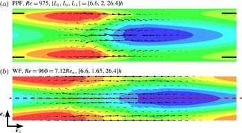
Figure 7 shows the mean structure of turbulent bands in PPF and in its stress-free counterpart. Excluding the boundary layers of PPF, there is very good agreement between the structures in these flows. By construction, the lower half of figure 7(b) is identical to figure 3(b). The lower half of figure 7(a) also strongly resembles figure 3(a). The resemblance between turbulent bands in these two flows solidifies the prevalent view of PPF as two PCFs (Waleffe Reference Waleffe2003; Tuckerman et al. Reference Tuckerman, Kreilos, Schrobsdorff, Schneider and Gibson2014).

Figure 6.

Doubled Waleffe flow seen as an approximation to the interior of plane Poiseuille flow. Shown are streamwise velocity profiles for PPF (solid/red) and WF (dashed/blue and grey) in the uniformly turbulent regime (PPF: $\mathit{Re}=1800$ and WF: $\mathit{Re}_{w}=500$ ). Plotted are (a) laminar flow, (b) deviation of mean turbulent profile from laminar flow and (c) mean turbulent profile. The $y$ -scale of WF is non-dimensionalised using $H=2h/0.825$ to align its stress-free boundaries (dashed horizontals) with extrema of the PCF deviation profile in (b). WF velocities are likewise scaled by $V=2U/0.825^{2}$ so that both flows have same average laminar shear in (a). Data are from simulations of 2000 advective time units for $[L_{x},L_{y},L_{z}]=[12,2,10]h$ .

The low-order model of Waleffe flow derived for PCF in § 3 carries over in a straightforward manner to PPF and is therefore not shown. A five-mode model of wall-bounded PPF was derived by Lagha (Reference Lagha2007) and used to study spot growth.

Figure 7.

Comparison of bands between plane Poiseuille flow (a) and doubled Waleffe flow (b). Contours are for streamwise velocity $[-0.4,0.4]$ , and arrows for in-plane velocity. Domain size and Reynolds number for PPF were chosen to match with the (rescaled) WF bands plotted in figure 3(b). This comparison excels near the midplane in PPF and confirms that PPF can be viewed as two plane Couette flows; compare figures 7(a) and 3(a).

5 Stress-free pipe flow

Finally, we turn to pipe flow (PF), the third canonical wall-bounded shear flow, in which intermittency takes the form of puffs. We introduce a Bessel function body force that drives a laminar flow confined by cylindrical stress-free boundaries:

where $k_{0}^{\prime }\approx 3.83$ is the first non-zero root of $J_{0}^{\prime }$ .

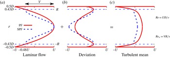
Simulations are conducted using openpipeflow.org (Willis & Kerswell Reference Willis and Kerswell2009) adapted to enforce stress-free conditions on the pipe walls. As before, we first consider uniform turbulence (figure 8) and non-dimensionalise our stress-free flow to match the turning points in the deviation. This results in $R=0.86\,D/2$ , $V=0.86^{2}\times 2U$ and a Reynolds number

where $D/2$ is the pipe radius and $2U$ is the maximum laminar speed. Like the cosine forced version of PPF, stress-free pipe flow undergoes a linear instability at low Reynolds number ( $\mathit{Re}\approx 340$ ), below the existence range of turbulence. Therefore to study laminar–turbulent intermittency (here turbulent puffs) we impose the symmetry

which stabilises the laminar flow. We will only present results from $\boldsymbol{R}_{3}$ here but alternative choices (e.g. two and four) produce comparable results.

Figure 8.

Stress-free pipe flow (SPF) seen as an approximation to the interior of pipe flow (PF). Shown are streamwise velocity profiles for PF (solid/red) and SPF (dashed/blue) in the uniformly turbulent regime (PF: $\mathit{Re}=3000$ and SPF: $\mathit{Re}_{w}=1900$ ). Plotted are (a) laminar flow, (b) deviation of mean turbulent profile from laminar flow and (c) mean turbulent profile. The $r$ -scale of SPF is non-dimensionalised using $R=0.86D/2$ to align its stress-free boundaries (dashed horizontals) with extrema of the PF deviation profile in (b). SPF velocities are likewise scaled by $V=2\times 0.86^{2}U$ so that both flows in (a) have the same average laminar shear. Data are from simulations of 2000 advective time units for pipes of length $5D$ .

Figure 9.

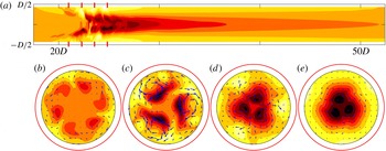
A turbulent puff in stress-free pipe flow. (a) Streamwise velocity along the pipe (only partial pipe shown) and (b–e) $(r,{\it\theta})$ slices along the pipe (indicated by red lines in (a)) with arrows of in-plane velocity. Motivated by figure 8, the red circles show the location of the walls for the corresponding wall-bounded flow, highlighting the absence of boundary layers in the stress-free case. Nine contours are used for streamwise velocity varying in $[-0.86,0.48]$ .

In this symmetry subspace, turbulent puffs are found for stress-free pipe flow over a range of Reynolds numbers $\mathit{Re}\in [2400,3500]$ ; an exemplar is plotted in figure 9. For conventional rigid-wall pipe flow in this subspace, turbulent puffs are first observed at $\mathit{Re}\approx 2400$ , an increase from $\mathit{Re}\approx 1750$ (Darbyshire & Mullin Reference Darbyshire and Mullin1995) for no imposed symmetry. The structure and length scales of these puffs are comparable with their wall-bounded counterparts. Excitation occurs upstream (figure 9 b,c), generating fast and slow streaks that slowly decay downstream (figure 9 e). The success of model Waleffe flow combined with the low-azimuthal-resolution model of Willis & Kerswell (Reference Willis and Kerswell2009) suggests that a model with one spatial dimension ( $z$ ) is possible. However, the complexity of cylindrical coordinates, particularly the coupled boundary conditions, prevents further work at this time.