Voter mobilization campaigns are a central part of democratic elections. In the 2000 general election, for example, the Democratic and Republican parties spent an estimated $100 million on such efforts urging likely supporters to vote (Dao 2000). Not only do political parties engage in strategic mobilization of targeted voters, but also many public interest groups make nonpartisan appeals. In particular, telephone canvassing has been one of the most widely used voter mobilization strategies. Yet in their landmark study of a field experiment, Gerber and Green (2000) found that phone calls encouraging people to vote reduce turnout by five percentage points on average. Indeed, their experiment implies that among single-voter households, phone calls reduce turnout by 27 percentage points. Gerber and Green (2000, 660) describe the negative effect of get-out-the-vote calls as “one of the most surprising results to emerge from our experiment.” Not only does this finding go against the conventional wisdom in the literature, but also it throws into question why so many millions of dollars are spent on telephone canvassing for every election.
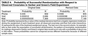
In this article, I introduce statistical methods into political science research that enable us to uncover the discrepancies between designed experimental protocols and actual implementation. The same methods can be used to analyze nonexperimental data, where deviations from randomization are to be expected. Application of this methodology to Gerber and Green's data shows that the negative finding about telephone canvassing originates from errors that occurred during implementation of the experiment. These errors resulted in the failure of randomization that would have been difficult to detect (and indeed were not detected) without my methods. For example, among single-voter households, those individuals who did not vote in the last election were more likely to be assigned phone calls. A statistical test I introduce shows that under the procedure specified in their original article, the pattern of incomplete randomization observed in the data would only occur with a probability of about one in 300 million. This and other implementation failures contributed to the highly implausible result that get-out-the-vote calls decrease turnout by 27 percentage points among single-voter households. Moreover, Gerber and Green's article used incorrect treatment and control groups in their analysis. Since the estimation of causal quantities necessarily involves the comparison of these two groups, their reported estimates turn out to be incorrect.
In order to correct these problems, I apply a more appropriate statistical method, propensity score matching, that has become standard in other fields when estimating the causal effects of nonrandom treatments (see Horiuchi, Imai, and Taniguchi (2005) for an example of analyzing a field experiment with completely randomized treatment assignment). The main advantage of matching is that it does not require restrictive functional form assumptions common to usual regression analysis (see Ho, Imai, King, and Stuart 2004). This method literally matches each observation in the treatment group (e.g., those receiving phone calls) with observations in the control group (e.g., those not receiving phone calls) whose observed characteristics are otherwise similar. The method, thus, constructs control and treatment groups that are systematically different only with respect to whether they received treatment. The propensity score facilitates the use of matching in multivariate settings where one needs to match on many variables (Rosenbaum and Rubin 1983).
The results of this analysis reverse Gerber and Green's finding to show that get-out-the-vote calls increase turnout by about five percentage points on average. This result is consistent with previous experimental studies on the topic (e.g., Adams and Smith 1980, Eldersveld 1956, and Miller, Bositis, and Baer 1981), all of which found that such calls increase voter turnout. Moreover, it corroborates the evidence from a subsequent field experiment by the same authors (Green and Gerber 2001).
Despite the clear evidence in their data, Gerber and Green (2000) are careful not to overstate the negative impact of phone calls.1
Gerber and Green (2000, 660) write, “Given our initial expectation that telephoning increases turnout, we take this [negative] result to mean that the null hypothesis of no effect cannot be rejected using a one-tailed test.”
They do, however, declare phone calls to be ineffective. Moreover, in another article, Gerber and Green (
2001, 80) offer an explanation for the negative impact of phone calls, saying that “it is conceivable that the phone call irritated some people and made them slightly less likely to vote.”
2 This study is based on a field experiment that Gerber and Green conducted in West Haven at the same time as the New Haven study. See the section Implementation Errors and Remaining Discrepancies for more information about the relationship between the two studies.
The policy implication of their finding is that money should not be spent on telephone canvassing.
I also demonstrate that Gerber and Green (2000) may have been too quick to dismiss the utility of mailings. The authors assumed that everyone who was sent postcards received and read them. As a consequence, when assessing the relative cost effectiveness of postcards, Gerber and Green incorrectly compared the effect of sending postcards with the effect of visits on those who were home and talked with the canvasser. I show that once the appropriate comparison is made, mailing postcards can represent a cost-effective alternative to sending canvassers directly to households.
By finding and correcting the errors of Gerber and Green's study, therefore, this article makes two methodological contributions that are relevant to field experiments in general: introduce statistical methods that enable us to find problems in experimental designs, and illustrate how statistical methods can correct problems like these wherever they exist.
Statistical Methods Are Essential for Field Experiments
The methodological issues that arose in Gerber and Green's experiment have important implications for field experiments in general. Long after the first such experiment was conducted by Gosnell (1927), field experiments have recently become an increasingly popular approach in the discipline (e.g., Howell and Peterson 2002 and Wantchekon 2003). This is an important development for political science because field experiments are a promising method that overcomes many of the limitations of purely observational studies.
However, Green and Gerber (2002, 810–11) go too far to conclude that with field experiments, “rudimentary data analysis replaces scores of regressions, freeing the researcher from the scientific and moral hazards of data mining.”3
Using the study of the effects of campaign contributions on political access as an example, Green and Gerber (2002, 810–11) write, “Rather than launch a complex multivariate analysis of the flow to and from donations and access, the researcher may obtain an unbiased assessment of the average treatment effect merely by cross-tabulating access by the size of contribution. Rudimentary data analysis replaces scores of regressions, freeing the researcher from the scientific and moral hazards of data mining.”
If field experiments work perfectly—with perfect random selection of a large sample and completely randomized assignment of treatment among individuals—and, in addition, the empirical relationships are unambiguously strong, then sophisticated statistical analysis may be unnecessary. However, precisely because field experiments take place in the real world, such perfection is almost never achieved in practice.
The problems encountered by Gerber and Green (2000) highlight the difficulty of implementing experiments in the field. Statistical methods are essential for detecting and correcting such unintended, but not entirely unforeseeable, complications that arise in field experiments. The point of the article is not, however, to discourage field experiments as infeasible. The lesson is that only with appropriate statistical methods can we draw valid inferences from field experiments. Such efforts are worth undertaking precisely because field experiments may give us a better understanding of causal processes.
Implementation Errors and Remaining Discrepancies
The statistical methods introduced in this article detected the implementation errors in the field experiment of Gerber and Green (2000). I sent the first draft of this article to Gerber and Green, pointing out what appeared to be their implementation errors. This prompted the authors to take another look at their original data. After they investigated potential implementation errors, Gerber and Green graciously documented what went wrong and posted a new data set on their Web site. On the same Web site, they published a retraction of some numerical results from their ASPR article and a replacement for the key table. Further questions from my analysis led to additional updates of the revised data.
According to their latest account, Gerber and Green sent two separate lists of registered voters to the phone bank that they hired for telephone canvassing. The phone bank mixed up one of the lists with that for another field experiment conducted by Gerber and Green (Public Opinion Quarterly, 2001) in West Haven. Among the mistakes that resulted, some voters received an appeal message asking them to donate their blood rather than a message asking them to cast their ballots. Consequently, the experiment was not implemented in the way it was described in the original article.
In this article, I present the methods used for detecting the errors of Gerber and Green's experiment. I also apply the same methods to the most recent data and conclude that the failure of implementation is still apparent with the new coding scheme. Indeed, a statistical test shows that the incomplete randomization observed in the revised data would occur only with a probability of about one in 2 billion. Given that the implementation errors exhibit systematic patterns, the treatment assignment of the revised data appears to be even less randomized than the original data. I hope that in their response to this article Gerber and Green will track down and report the source of the randomization problems in both data sets.
Finally, I analyze the revised data with a more appropriate statistical method. Whichever data are used, the substantive conclusion remains the same: get-out-the-vote calls increase turnout, whereas Gerber and Green's analysis implies otherwise. Nevertheless, Gerber and Green's data correction brings their estimates closer to mine. This is not surprising because the implementation errors of field experiments can be fixed in two ways: by adjusting statistically as I demonstrate in this article or by correcting the data as Gerber and Green did. When possible, correction of data is generally preferable to ex post statistical adjustments. Once the experiment has been conducted, however, data correction by the experimenter alone often fails to fix all of the errors that occurred during implementation. That is, there is no way to change the fact that randomization failed in Gerber and Green's experiment. Therefore, further statistical adjustments are necessary for the revised data as well.
ADVANTAGES OF RANDOMIZED FIELD EXPERIMENTS
A central goal of scientific inquiry is to make causal inferences. In the physical sciences, experiments are essential for this purpose. In contrast, for many political scientists, analysis of observational data and comparative case studies have been the more common approaches, and relatively few researchers conduct experiments. Recently, Green and Gerber (2002, 831) have characterized the state of the discipline as resembling “monocrop agriculture, efficiently generating prodigious quantities of nonexperimental research but deeply vulnerable to an experimental intrusion that could consume the stock of received wisdom.”4
Gerber, Green, and Kaplan (2002, 1) conclude that “at some point, the only possibility of further learning comes from experimentation.”
Indeed, the experimental approach can often provide more insight into causal processes with fewer arbitrary assumptions than would be necessary in observational studies (e.g., Kinder and Palfrey
1993).
Gerber and Green advocate field experiments, which are attempts of randomized interventions into real-world settings, as the best way to conduct empirical political science research. Although laboratory experiments offer greater control, conclusions based on such studies are often difficult to generalize. In contrast, field experiments combine real-world settings with a significant level of control over experimental design and produce more generalizable results.
The Role of Randomization
Establishing causality involves the comparison between what actually occurred and what might have happened under different circumstances. The fundamental problem of causal inference is that we never observe the counterfactual scenario (e.g., Holland 1986 and King and Zeng 2003). For example, in order to measure the causal effect of British colonial rule on the postcolonial economic development of India, one must estimate the economic growth of India if it had not been ruled by the British empire. Answering such counterfactual questions is difficult, but doing so is necessary to address important research topics in political science.
More formally, let Yi(Ti=t) be the potential outcome under the treatment status, t, for unit i. Here, Ti is an indicator variable that is equal to one if this unit received the treatment and zero otherwise. Then a treatment effect for unit i, TEi, can be defined as
If a unit belongs to the treatment group, we only observe Yi(Ti=1), and the counterfactual outcome if the same unit had not received the treatment, Yi(Ti=0), is unknown. In the context of voter mobilization, if a voter received a get-out-the-vote call, we never know for certain whether he or she would have voted had the call not been received. Therefore, the validity of causal inference rests on how reliably we estimate the potential outcome under a counterfactual scenario. This is true even in experimental settings since we cannot repeat the identical experiment on the same unit in the same environment.
One way to achieve this goal is to form an appropriate control group that is similar to the treatment group in all characteristics except for the treatment status. In experiments, randomization plays a critical role in obtaining such a control group. By giving a treatment to randomly selected units, all characteristics of the treatment and control groups, except for whether they received the treatment, become similar as the sample size increases. As a whole, the two groups are essentially identical if there is a large sample. In this manner, randomization equalizes unobserved as well as observed characteristics of the two groups. If treatment is completely randomized, we can simply use the mean difference of the observed outcome between the treatment and the control groups as an unbiased estimate of the average treatment effect. A serious limitation encountered in observational studies, in contrast, is that researchers do not possess the powerful tool of randomization (e.g., Achen 1986).
Quantities of Interest in Field Experiments
In many field experiments, the distinction between assignment of treatment and receipt of treatment is critical because researchers can often randomize the former, but not the latter. In the field, not everyone assigned the treatment by researchers actually receives it. In addition, some of those who are not assigned the treatment may receive one. Because of this noncompliance problem, the estimation of treatment effects in Equation (1) requires additional assumptions that allow for further statistical adjustments.
The difficulty of estimating treatment effects leads many to estimate another causal quantity, known as the Intention-To-Treat (ITT) effect. Unlike the treatment effect, the ITT effect does not take into account whether those assigned the treatment received it. That is, the ITT effect represents the effect of treatment assignment rather than treatment itself. Unlike the treatment effect, the ITT effect is relatively easy to estimate so long as the treatment assignment is randomized. Indeed, for some cases when the information about who actually received the treatment is unavailable, one can only estimate ITT effects. Formally, let Zi be the treatment assignment indicator, which is equal to one if unit i is assigned the treatment and zero otherwise. Then, the ITT effect for unit i can be defined as
where Ti denotes whether the treatment was actually applied and is equal to either 0 or 1.
Figure 1 shows the diagram of typical randomized field experiments. Here we assume that subjects would never receive the treatment if they are not assigned one; i.e., Ti=0 if Zi=0. Because of the selection bias due to noncompliance described above, we cannot directly compare those who received the treatment with the units of the control group. The ITT analysis is valid, on the other hand, as long as the treatment assignment group is compared with the control group. Furthermore, in many cases we can only estimate the treatment effect for compliers (i.e., those who would receive the treatment only if they were assigned one), and to do so, we need to identify compliers in the control group. Once we identify such individuals, we can use them to estimate the average potential outcome under no treatment for compliers.
Diagram of a Typical Randomized Field Experiment with Noncompliance
ITT effects may substantially differ from treatment effects. Consider a hypothetical example where an international organization plans an AIDS prevention campaign in Africa and must choose from two proposals. The first proposal is to distribute educational pamphlets to local high schools. The second proposal is to put up an educational message on roadside billboards. The first policy would have the greatest treatment effect if those pamphlets are actually read by students at school. However, it is questionable whether school teachers will read them to students. It is also possible that the youth in schools are less likely to be infected with AIDS in the first place. Therefore, one would expect the ITT effects of this proposal to be low despite its potentially high treatment effect. In contrast, the billboard advertisements may have a higher ITT effect because they are more likely to be read by the target population. Thus, policy-makers may prefer the proposal to use billboard advertisement even if it has a smaller treatment effect.
ITT effects are often useful for policy makers who are interested in the cost effectiveness of policy programs. In contrast, academic researchers may care more about treatment effects in order to learn about underlying causal processes. For example, electoral candidates may want to know about how many visits or postcards are necessary to increase voter turnout by one percentage point. In this case, it is not necessary to know how many voters actually talked to canvassers or read postcards. On the other hand, political scientists, who want to assess the relative effectiveness of various canvassing methods need this extra information. Even when personal canvassing seems less effective, for example, it may only appear ineffective because voters are more difficult to reach by visits than by postcards. Hence, the different compliance rates for the two methods become critical.
THE NEW HAVEN VOTER MOBILIZATION STUDY
In this section, I replicate and extend Gerber and Green's analysis of the voter mobilization study. Gerber and Green (2000) designed and conducted an experiment where registered voters in randomly selected households of New Haven were encouraged to vote in the 1998 general election by means of personal visits, phone calls, and postcards. They then examined voting records and analyzed which strategies had increased voter turnout. In addition to the voting record of the 1998 election, the data include covariates that describe the following characteristics of each registered voter: number of registered voters in the household (one or two), age, party affiliation (registered Democrats, registered Republicans, or others), voting record in the last general election (voted, did not vote, or was not registered for 1996 election), and ward of residence in New Haven (29 wards).
Inefficient Experimental Design
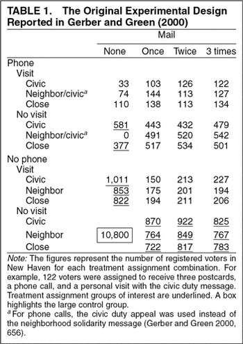
Table 1 shows the unusually complicated experimental design of the original study with the substantial overlap of different treatment assignments. Over 40% of voters in the sample were assigned more than one treatment. For example, 122 voters were assigned to receive three postcards, a phone call, and a personal visit with the civic duty message. Further variation in the nature of the treatment was possible because Gerber and Green used three different appeal messages; civic duty, neighborhood solidarity, and close election. The authors note that the neighborhood solidarity message was not used for phone calls (Gerber and Green 2000, 656). Altogether, this design produced a total of 45 different treatment combinations and their corresponding potential outcomes. Such complex experimental design leads to the inefficient estimation of treatment effects unless one makes arbitrary assumptions. This is unfortunate since the advantage of experimental methods is to avoid additional assumptions that are often necessary in observational studies. For example, Gerber and Green (2000) assume that the effect of telephone canvassing remains the same regardless of whether voters have received other treatments. However, phone calls may not increase the probability of voting as much for those voters who already have received a personal visit. Furthermore, the timing of contact differs from one canvassing method to another and this variation was not randomized; e.g., phone calls were made during the three days prior to the election, whereas personal visits were made over a period of four weeks. Such systematic differences in the administration of multiple treatments will yield incorrect inferences unless properly controlled in the analysis.
Incorrectly Identified Treatment Assignment and Control Groups
Gerber and Green (2000) also incorrectly identified the treatment assignment and control groups used in their field experiment and, as such, failed to estimate their causal quantities of interest. For example, when estimating the marginal effect of phone calls, Gerber and Green used the treatment assignment group that includes those who were also assigned other treatments such as personal visits and postcards (the upper two rows in Table 1). Their control group included those voters who were assigned other treatments (all categories in the bottom two rows in Table 1). In order to correctly estimate the treatment and ITT effects, the appropriate control group should consist solely of the 10,800 voters who were assigned no treatment and hence received no intervention. Likewise, the members of the treatment assignment group for phone calls should not include those who were assigned any other treatment.
This implies that the ITT and treatment effects reported in Gerber and Green (2000) are confounded by the effects of other treatments.5
This may lead to the underestimation of the treatment effect since the control group used by Gerber and Green includes those who received other treatments. Many voters in the treatment assignment group were also assigned one or more of the other treatments. The treatment effects are likely to be small for those who have already received other treatments.
In experiments, an appropriate control group is critical to ensure internal validity (e.g., Campbell and Stanley
1963). In principle, it is advisable to minimize the number of treatments in field experiments. Although factorial designs may be feasible in laboratory experiments, additional complications such as noncompliance make it difficult to estimate the effects of multiple overlapping treatments in field experiments. In this article, I focus on the marginal effects of each treatment rather than their interaction effect, as the latter would involve additional assumptions and few data are available to estimate such quantities.
Experimental Design Based on the Revised Data
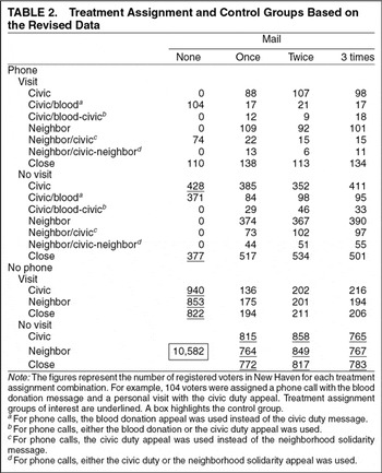
As noted above, the analysis in the initial draft of this article detected the implementation errors and led to the subsequent revisions of the original data. Table 2 shows the treatment assignment and control groups based on the most recent data and Gerber and Green's latest version of their experimental design. The total number of treatment combinations is now seventy, making the experimental design even more complex. For the analysis of the revised data, I correct the treatment group for telephone canvassing to include only those voters who were assigned no other treatment. I also exclude those who were possibly assigned the blood donation messages. This yields the total of 428 voters with the civic duty appeal and 377 individuals with the close race message. The new control group consists of 10,582 voters who were assigned no treatment.
The analysis of the revised data reveals discrepancies between Gerber and Green's description of the implementation errors and the altered coding scheme. For example, on their Web site they describe one of their errors as follows: “Subjects who would have received Civic Duty mail or personal appeals received phone appeals requesting a Blood Donation” (see footnote 4). Although this error should not affect the control group of those who were assigned no treatment in the first place, the revised control group has about 300 voters fewer than the original group. Such remaining inconsistency calls for further clarifications about the coding changes beyond what is currently documented.
ANALYSIS ASSUMING COMPLETE RANDOMIZATION WITH CORRECTED TREATMENT ASSIGNMENT AND CONTROL GROUPS
With the corrected treatment assignment and control groups, I reestimate the average ITT and treatment effects by applying the statistical method used in Gerber and Green (2000), which assumes complete randomization of treatment assignments.
Estimation of the ITT Effect
Under the assumption of complete randomization, the treatment assignment is independent of all observed and unobserved individual characteristics. Therefore, the difference in the sample means of the treatment assignment and control groups is an unbiased estimate of the average ITT effect. Namely,
where N1=[sum ]i=1N Zi is the size of the treatment assignment group N0=[sum ]i=1N (1−Zi) is the size of the control group, and N=N0+N1.6
In the case of phone calls, for example, N1=958 and N0=10,800.
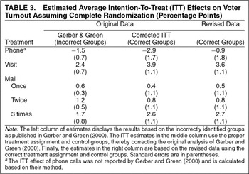
Table 3 shows the results of the ITT analysis using the correct treatment and control groups. First, the corrected ITT analysis in the middle column confirms the conclusion of Gerber and Green (2000) that personal canvassing is the most effective method for increasing voter turnout. Second, get-out-the-vote calls have a significant negative effect on turnout. Using the appropriate treatment assignment and control groups does not change the odd finding of the original article that telephone canvassing reduces voter turnout.
As one would expect, altering the data also changes the estimates. The analysis of the revised data with correct groups (in the right column) suggests that the overall ITT effect of phone calls is only slightly negative, with a larger standard error. In the next section, however, I show that the data correction alone does not solve the entire problem. In principle, the implementation errors of field experiments cannot be fixed by the experimenter after the fact without statistical adjustments.
Mail canvassing also mobilizes voters. (Gerber and Green 2000, 661) argued that “even if the effective marginal costs of canvassing were doubled, face-to-face mobilization would still be cost effective.” This conclusion, however, is based on their assumption that all voters who were sent postcards actually received and read them (659, fn 10). Such an assumption is not warranted because many cards may not have reached a voter due to changes of address or may have been discarded unread as junk mail. As a consequence, Gerber and Green (2000) underestimated the effectiveness of sending postcards by incorrectly comparing the estimated ITT effects for postcards with the estimated treatment effects for visits. The ITT effect may well be the most relevant for the evaluation of cost effectiveness in this case, but the comparison that was made here was inconsistent. The valid comparison of different canvassing methods must be made using the same estimand to evaluate their relative effectiveness.
In contrast, the corrected ITT analysis in the middle column of data in Table 3 makes the appropriate comparison of the ITT effects across the three mobilization strategies. Given the relatively low cost of sending postcards compared to visiting each voter's residence, policy-makers might reasonably prefer to use postcard mailings as a cost-effective method to raise voter turnout. The corrected analysis also indicates that sending a postcard three times is much more effective than mailing it once or twice. This provides evidence against the assumption of Gerber and Green (2000) that the effect of mail canvassing is linear in the number of postcards sent.
Instrumental Variables Estimation of Treatment Effect
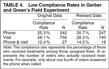
Moving from the estimation of ITT effects to that of treatment effects necessitates attention to compliance with treatment assignment. In field experiments, noncompliance often occurs because researchers cannot force everyone assigned a treatment to receive it. Table 4 shows that in Gerber and Green's experiment, only one fourth of those assigned a treatment actually received it. The noncompliance exists mostly because voters were not at home (or were at home but unwilling to talk to a canvasser) when they were visited or telephoned. Furthermore, among 217 voters who were assigned a phone call and a visit, only 27 of them actually received both treatments, illustrating the difficulty of estimating the effect of multiple treatments in field experiments. Note the significant difference in compliance rate for phone calls between the original and the revised data. This implies that the coding changes did not occur randomly and that systematic changes have been made to the original data.
Instrumental variables (IV) estimation is a well-known statistical method that identifies average treatment effects by focusing on those who would receive a treatment only if assigned (e.g., Angrist, Imbens, and Rubin 1996).7
Some argue that the treatment effect for the entire population is a more meaningful quantity (e.g., Balke and Pearl 1997). The inefficient design and high noncompliance rate of Gerber and Green's experiment make estimating such a quantity difficult. I computed the nonparametric bounds of the average treatment effect for personal visits and phone calls and found that they are [−27.9%, 43.9%] and [−28.1%, 46.6%], which implies that the data from this field experiment are almost entirely uninformative about this quantity of interest.
An “instrument” is a variable that satisfies an assumption referred to as the
exclusion restriction; i.e., the instrument influences the outcome only through its effect on the treatment. In other words, the instrument cannot have any direct or indirect effect through variables other than the treatment variable. In field experiments, the assignment of treatment, if completely randomized, may serve as an ideal instrument.
8 To be precise, this is not always the case. In Gerber and Green 2000, for example, the existence of potential spillover effects within households will violate this assumption even if the assignment is completely randomized. However, since Gerber and Green's replication data do not contain the information about which household each voter belongs to, it is impossible to conduct the household-level analysis.
In Gerber and Green's study, the fact that voters were assigned telephone canvassing via random numbers generated by a computer is unlikely to affect anything other than the probability of their receiving phone calls. Formally, the exclusion restriction can be written
Yi(
Ti =
t,
Zi = 1) =
Yi(
Ti =
t,
Zi = 0) for
t = 0,1 where
Zi is the indicator variable for treatment assignment.
The IV estimator is biased in small samples, but it consistently estimates average treatment effects for compliers in large samples when treatment assignment is completely randomized. Gerber and Green (2000) employ this approach to estimate the marginal treatment effects of telephone calls and personal visits for the subgroup of those who received an assigned treatment. The ITT effect divided by the compliance rate gives the IV estimate of complier average treatment effect. Namely,
where the denominator represents the estimated compliance rate as appears in Table 4.
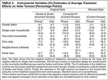
Table 5 presents the IV estimates of the average treatment effects of telephone and personal canvassing.9
Gerber and Green used the two-stage least squares and the two-stage probit regression for phone calls since the phone treatment assignment was correlated with the postcard assignment. Both are variants of IV estimation presented here. See, e.g., Angrist and Imbens 1995 for a complete discussion.
Gerber and Green (
2000) found that get-out-the-vote calls have a significant negative effect of five percentage points on turnout.
10 While Gerber and Green's two-stage least-squares analysis (with all covariates) indicates a smaller negative effect, their two-stage probit analysis shows that the effect of phone calls is about negative five percentage points and statistically significant.
Moreover, their inappropriate use of overlapping treatments obscured greater problems. Correcting the treatment assignment and control groups makes the effect even larger, reaching −12 percentage points with a standard error of seven percentage points. These IV estimates based on the original data suggest that get-out-the-vote calls encouraging people to vote discourage them from casting their ballots.
Note that although the negative effect for single-voter households seems to persist in the revised data, the estimated overall effect of phone calls is now small with a large standard error. This is similar to the situation of ITT estimates mentioned above in that the data correction brings Gerber and Green's estimates closer to positive effects. As I show below, however, data correction alone is not sufficient to fix the implementation errors.
Finally, the corrected IV estimates for personal visits are much greater than those from the original analysis for both original and revised data, reaching to an increase of more than 10 percentage points in turnout. This significant difference is solely due to the correction of treatment assignment and control groups. This is clear evidence against the assumption of Gerber and Green (2000, 660) that the effects of different canvassing methods are constant and additive.
METHODS FOR EVALUATING THE IMPLEMENTATION OF FIELD EXPERIMENTS
While the IV method is useful in many situations, the validity of its use relies on the key assumption that treatment assignment is completely randomized. Below, I show that this assumption was violated in Gerber and Green's experiment and that the violation led to their negative finding about telephone canvassing. Indeed, I now demonstrate, with statistical tests I introduce, that the pattern of incomplete randomization observed in Gerber and Green's original data would occur with a probability of less than one in 300 million. These results led to the discovery of the implementation errors of their experiment.
The fact that the errors did not occur randomly is another indication of failed randomization in this experiment. For example, Gerber and Green's revisions of the original data increased the overall rate of compliance for phone calls by five percentage points (see Table 4). This difference is statistically significant (p-value, 0.01), implying that the implementation errors systematically affected those individuals who were more likely to answer the phone when called. Thus, IV estimation, which assumes complete randomization, is not an appropriate method to analyze either the revised or the original data.
Detecting the implementation errors of field experiments is generally a difficult task. The main challenge arises from the fact that statistical tests based on the observed data cannot guarantee that the treatment assignment is randomized with respect to unobserved variables. For this reason, it is advisable to gather as many important covariates as possible when designing field experiments. The validity and efficiency of resulting estimates can be improved by incorporating covariates in the randomization procedure (e.g., using stratification methods) as well as in the data analysis.
Assessing Sensitivity of IV Estimates
Examination of different subgroups is one way to check the robustness of IV estimates. Such analysis can be informative since the IV estimate of the overall treatment effect is equal to the weighted average of estimates for different subgroups. The analysis shows that the large negative effect among single-voter households underlies Gerber and Green's pessimistic conclusion about the effect of telephone canvassing. In particular, the overall estimate of negative five percentage points reported in Gerber and Green (2000) is largely due to the significant negative effect of 14 percentage points found for single-voter households, with a standard error of four percentage points.11
Gerber and Green (2000, 658) report the results of the separate subgroup analysis for personal canvassing but not for phone calls.
Similarly, the corrected IV estimate for this subgroup is −27 percentage points (with a standard error of 10 percentage points), which leads to an overall effect of −12 percentage points. Large negative effects for single-voter households contrast with positive effects for two-person households. For the revised data, the gap between the two subgroups is also apparent; i.e., −13 percentage points for single-voter households and positive seven percentage points for two-voter households (with standard errors of nine and eight percentage points, respectively).
Looking closely at subgroups that received different messages also reveals large negative IV estimates for the effect of get-out-the-vote calls. The corrected IV analysis for the original data shows that both civic duty and close race messages significantly reduce turnout, by more than 10 percentage points.12
Applying Gerber and Green's incorrect groups, I also find that the civic duty appeal has a significant negative effect of eight percentage points, while the effect of the close race message is only slightly negative.
Although the corresponding standard errors are larger, the analysis of the revised data reveals even larger differences among the appeal messages; the close race message
reduces turnout by 12 percentage points, whereas the civic duty appeal
increases turnout by five percentage points. The inconsistency of the estimates across data sets as well as subgroups raises questions about the validity of conclusions regarding the effect of telephone canvassing.
Detecting Incomplete Randomization
Although it is generally difficult to check the randomization with respect to unobserved variables, the experimental design of Gerber and Green (2000) allows for such a test. In particular, both personal visits and phone calls are supposed to be assigned with randomly selected appeal messages: civic duty, neighborhood solidarity (not used for phone calls), and close election. If the assignment of appeal messages is random, one should see no systematic difference in compliance rates among different messages.13
The test assumes that the content of messages does not affect compliance. This assumption may be justified because all messages have the identical opening script. Also, the scripts are relatively short; telephone scripts lasted only for about 30 seconds (Gerber and Green 2000, 656).
This is because the randomization would prevent one message from being assigned to a group of people who are more likely to receive the treatment. Since the probability of voters being at home and willing to talk to a canvasser when called or visited depends on their unobserved characteristics as well as their observed ones, this test allows us to check the balance of unobserved voter characteristics. (“Balance” refers to a similar distribution for a variable in two subgroups.)
This analysis reveals that for phone calls, those who were assigned the close race message are on average about 10 percentage points more likely to answer a call than those who were assigned the civic duty appeal (p-value, 0.00073). For personal visits, one finds no systematic variation in compliance rates among different appeal messages; Pearson's χ2 test shows that one cannot reject the null hypothesis of equal compliance rate for all three appeal messages (p-value, 0.71).14
The result holds even when looking at the incorrect treatment assignment and control groups used in the original analysis. The mean difference for telephone canvassing is five percentage points (significant at the 0.01 level), while for personal canvassing differences across messages are not significant.
The different compliance rates for phone calls indicate the kind of nonrandom treatment assignment that could also explain the negative effects observed in Gerber and Green's IV analysis.
Even when it is impossible to check the randomization with respect to unobserved variables, one can conduct tests for observed variables. I apply the following method, which can be used to jointly test whether all observed covariates are balanced. First, I use a logistic regression to predict the assignment of each treatment using all covariates and their first order interactions as covariates.15
Due to the small size of its treatment group, for phone calls, only the past voting record and the household type variables are interacted with the other covariates.
If the model predicts treatment assignment well, this represents evidence that treatment assignment was not randomized. If treatment assignment is completely random, then assignment should be independent of
all covariates and
any function of those covariates.
16 If there are enough observations, other functional forms can be included in the model in order to allow for a more complex correlation structure.
Finally, I conduct the residual deviance test to examine whether these covariates together significantly help predict the treatment assignment (McCullagh and Nelder
1989, 119).
Table 6 presents the p-values of this test using the χ2 distribution. The p-values are very small, indicating the failure of randomization for all three treatments in both original and revised data. For example, the test for postcard mailings implies that the departure from randomization observed in Gerber and Green's data can occur only with a probability of one in 300 million. This probability is smaller for the revised data, reaching to one in 2 billion. (Note that a small sample size makes it harder to detect failure of randomization, so that the larger p-value for phone calls than for visits and mailings does not necessarily imply that randomization was more successful.) In sum, the test with respect to observed covariates also provides strong evidence that treatment assignment was not randomized in Gerber and Green's field experiment.
In field experiments, randomization of treatment assignment is not as easy to accomplish as one might expect. In practice, it is often difficult to randomize every aspect of each treatment. In Gerber and Green's experiment, personal canvassing was conducted over a period of four weeks before the election, whereas telephone canvassing took place over three days including the election day. Postcards were sent out during the two weeks before the election. Although a visit right before the election would have a greater effect than a visit one month before the election day, the timing of contact was not randomized. Likewise, the effect of different canvassers, if not randomized, can confound the effect of different canvassing methods. These examples illustrate the difficulty of randomization and potential confounding effects that threaten the validity of field experiments.
Finally, I investigate the sources of the negative finding about phone calls. Both Gerber and Green's analysis and the corrected IV analysis indicate that telephone canvassing has a large and negative effect on voter turnout among single-voter households. I find that for this subgroup the assignment of phone calls was not randomized with respect to the past voting record. In particular, only 42% of the treatment assignment group voted in the last election, whereas 47% of the control group voted (p-value, 0.05). The randomization for this group appears to be incomplete even with the incorrectly identified treatment assignment and control groups used by Gerber and Green.17
Compared with the control group, the treatment assignment group includes significantly more individuals who abstained in the last election. The mean difference is statistically significant at the 0.05 level.
Since those who voted in the last election are 40 percentage points more likely to vote in the current election on average, this difference contributes to the large negative effects of phone calls for single-voter households.
When One Should Not Use IV Estimation
The large bias of IV estimation that results from violation of the exclusion restriction is well documented (e.g., Angrist, Imbens, and Rubin 1996, 450). In particular, the bias is worsened when unbalanced variables are good predictors of the outcome variable and when a large number of noncompliers exist. Equation (4) illustrates these two conditions; the bias of the IV estimate is large (a) when the bias of the ITT estimate due to incomplete randomization is large and (b) when the compliance rate is low. (Recall that the IV estimate is equal to the ITT estimate divided by the estimated compliance rate.)
Gerber and Green's study fits both conditions for large bias. First, the unbalanced covariates (i.e., the voting record in the previous election) predict turnout well, which suggests that the bias in the estimated ITT effect is large. Furthermore, the compliance rate of this field experiment is low (about 25% for phone calls). This low compliance rate implies that if the ITT effect is biased by five percentage points, for example, then the bias of the IV estimate can be as large as 20 percentage points. Thus, the combination of a large bias in the ITT estimate and low compliance rate led to the puzzling finding that get-out-the-vote calls significantly decrease turnout.18
It is also important to note the finite sample bias and inefficiency of IV estimation (e.g., Bound, Jaeger, and Baker 1995). The small size of each treatment group in the New Haven mobilization study suggests the importance of finite sample consideration.
If one successfully randomizes the treatment assignment, the method of instrumental variables can give estimated treatment effects that are consistent in large samples. However, as the analysis of this section suggests, making this assumption in practice requires careful experimental design and successful implementation. In this case, the failure of randomization for telephone canvassing led to inaccurate causal inferences about the effects of get-out-the-vote calls in Gerber and Green (2000).
ANALYSIS WITHOUT ASSUMING COMPLETE RANDOMIZATION
The previous section showed that IV estimation was inappropriate for telephone canvassing given the incomplete randomization of treatment assignment. This calls for more general statistical methods to estimate the effects of nonrandom treatments. I apply propensity score matching to reduce the bias caused by nonrandom treatment.19
The estimand for the method of matching (i.e., the average treatment effect for the treated) can differ from that for IV estimation (i.e., the average treatment effect for compliers). In the New Haven mobilization study, however, the two estimands are equivalent because the treated did not include “always-takers,” who take the treatment even when they are not assigned the treatment (i.e., it is assumed that Ti=0 if Zi=0). See Angrist, Imbens, and Rubin 1996 for a complete discussion of this issue.
Matching is particularly useful for field experiments when randomization of treatment assignment is incomplete and important covariates are available. The basic idea of matching follows the logic of causal inference described earlier. The goal is to construct a control group as similar to the treatment group as possible. The method of matching finds two groups of subjects who have exactly the same observed characteristics except that one receives the treatment and the other does not. Since matching is a nonparametric method, it does not require the assumptions of usual regression analysis, (e.g., linearity and additivity), and hence it effectively reduces bias due to incomplete randomization.
The intuition behind matching resembles the traditional comparative case study method, which dates back to John Stuart Mill (1930/1843). Both approaches call for comparing cases that are very similar to each other except for the primary causal variable. This facilitates the evaluation of main causal effects in isolation by reducing the possibility of confounding effects from other variables. Although the comparative method has largely been used for qualitative studies, with the method of matching, quantitative and historical case studies can rest on a common ground of causal inference.
Selection Bias Due to Noncompliance
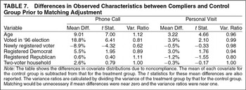
In field experiments, even when treatment assignment is completely randomized, the actual treatment group of compliers (Ti=Zi=1), as opposed to the treatment assignment group (Zi=1), is often different from the control group (Ti=Zi=0) in its characteristics. Table 7 illustrates the imbalance of observed covariates between compliers and the control group. The wide gap between the two groups indicates a significant selection bias that requires statistical adjustment. Compliers are older, are more Democratic, and have a better past voting record than the control group. A similar pattern is observed in the revised data. Estimates of treatment effects will be biased, unless one properly adjusts for these systematic differences between the two groups. Next, I explain how propensity score matching effectively reduces this selection bias.
Matching
The key assumption of matching is that compliers in the control group can be identified using their observed characteristics. In other words, the assumption implies that it is possible to estimate the counterfactual outcome under no treatment for a treated unit by using individuals from the control group who share the same observed characteristics. Formally, the counterfactual outcome under no treatment, Y(T=0), is assumed to be mean independent of the actual treatment status, T, conditioning on the set of observed control variables, X (e.g., Heckman et al. 1998),
Equation (5) implies that matching effectively reduces bias when important covariates are observed. Omitted variable bias is possible if the observed covariates, X in Equation (5), do not contain variables that affect both T and Y(T=0). The bias can be reduced, however, if those omitted variables are highly correlated with X. An advantage of matching is that this conditional independence assumption does not require parametric functional forms common to usual regression analysis such as linearity and additivity (see Ho, Imai, King, and Stuart 2004). If the assumption of Equation (5) is met, matching gives an unbiased estimate of average treatment effect by integrating over the distribution of X,
Propensity Score
Unfortunately, the application of exact matching becomes practically impossible as the number of control variables increases. For example, one might be able to match on voting records but not on age, ward of residence, etc. This curse of dimensionality implies that when many control variables are present, the standard regression analysis with its restrictive parametric assumptions often fails to pinpoint the correct functional relationship among the outcome and treatment variables. Even with the nonparametric method of matching, it is often difficult to find control units whose characteristics match exactly with a treated unit for all dimensions.
The use of the propensity score, defined as the conditional probability of receiving a treatment, aids the method of matching in such multivariate settings. It can be shown that this single variable summarizes relevant information in all observed control variables. Then, one only needs to match on this scalar variable, which is much more feasible than matching on the entire vector of X. More formally, Rosenbaum and Rubin (1983) show that conditioning on the propensity score, e(X)≡ Pr(T=1|X), is equivalent to conditioning on all observed characteristics, X. Hence, without additional assumptions, Equation (5) can now be replaced with
In most cases, however, the true propensity score is unknown to researchers. Thus, one must estimate it by modeling the actual receipt of treatment given observed covariates. The logistic regression can serve this purpose, although semiparametric and nonparametric methods can also be employed. Whatever model is used, the estimated model itself carries little causal interpretation and should be regarded as a tool to create a matched control group similar to the treatment group. If the propensity score is estimated properly, the distribution of observed covariates should be similar between compliers and matched control units. One has to change the model specification and reestimate the propensity score until this balance is achieved. An important advantage of propensity score methods over usual regression analysis is this diagnostic test that directly assesses the validity of causal inferences.
Although it is known to effectively reduce bias caused by nonrandom treatment (e.g., Dehejia and Wahba 1999), propensity score matching, like any other statistical method, risks bias due to omitted variables. That is, the method can only balance observed characteristics of the treatment and control groups. For example, if “politically interested” voters whose characteristics are not captured by observed variables are more likely to talk to a canvasser and go to polls, then propensity score matching may yield biased estimates. Estimates based on propensity score matching are also biased when the treatment group is too different from the control group.
In Gerber and Green's study, however, these problems are unlikely for three reasons. First, since the large control group roughly represents the population, we know that compliers exist in this group. Second, as shown later, I find many exact and close matches, indicating that the bias due to inexact matches is minimal. Third, when the covariates measuring important characteristics of subjects are available, propensity score matching is a powerful method for reducing bias. The availability of the voting record of the previous election is critical for successful matching in Gerber and Green's data. The ability to match on this variable allows further bias reduction by balancing unobserved variables that are correlated with the past voting record.
Although propensity score matching only uses a subset of the control group, the comparison of treated units with a matched control group gives more reliable estimates of treatment effects. When treatment assignment is not completely random and important covariates are observed, propensity score matching is the best available statistical method. Certainly, it is more appropriate than the method of instrumental variables used by Gerber and Green. Under these conditions, the method can also be applied to observational studies. Imai and van Dyk (2004) extend the propensity score to nonbinary treatments that are often encountered in observational studies. This generalization widens the potential applications of propensity score beyond experimental settings.
Application of Propensity Score Matching and Diagnostics
I apply the procedure referred to as nearest-neighbor propensity score matching to the New Haven voter mobilization study (Rosenbaum and Rubin 1985a, b). The goal is to select a group of voters of the 10,800 voters in the control group such that the distribution of covariates for the matched control group is similar to that for the treatment group. For each treatment unit, I select a control unit whose propensity score is the closest.20
I randomly order the treatment and control units before conducting matching.
If there is more than one voter with the same propensity score, I randomly select one of them. I repeat this procedure to obtain several matched control units for each treated unit; five matches for phone calls, yielding 1,210 selected control units, and three matches for personal visits and mailings (three postcards), yielding 2,268 and 7,125 matched control units, respectively. Increasing the number of matched control units generally improves the efficiency of resulting estimates because more observations are included in the analysis, but it will typically produce a greater imbalance of covariates between treated and matched control units, which in turn may lead to biased estimates. As shown below, different matching schemes can also be used for sensitivity analysis to detect this potential bias.
To estimate the propensity score, I use logistic regression starting with the specification where I include all available covariates as linear predictors. When this model does not balance all covariates, I search for an alternative specification by including additional terms to improve the balance.21
The model specifications for the original data are as follows. For phone calls, the household type variable is interacted with past voting record. For personal visits, the household type is interacted with the other variables except the new voter variable. Both models include the square term of age. For mailings, the household type is interacted with age, past voting record, and ward of residence variables. The model specifications for the revised data are as follows. For phone calls, the square term of age and the two interaction terms of the household type, one with the past voting record and the other with the new voter variable, are added. For personal visits, the interaction terms of the household type with the other variables except the past voting record are added. For mailings, the household type was matched first, and all first-order interaction terms are included.
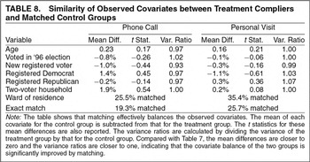
I use mean differences and variance ratios to investigate the resulting balance of covariates and determine model specification. Since all covariates except age of voters are indicator variables, these two statistics are generally sufficient to measure the similarity of the covariate distributions between treated and matched control units. The availability of such diagnostic tests for model specification is an important advantage of propensity score methods.
Table 8 shows that matching on the estimated propensity score successfully balances all observed covariates. The mean differences of all covariates between the treated units and the control-group individuals are not statistically significant and their variances are similar. In particular, propensity score matching significantly improves the balance of covariates compared with Table 7. I also find many exact matches. For phone calls, about one fifth of the matched control units share exactly the same values of all covariates with one of the treated units. That is, they live in a household with the same number of registered voters, are exactly the same age, have the same party affiliation, reside in the same ward of New Haven, and have the same voting record in the previous election. Similarly, in the case of personal visits, I find about one fourth of the matched control units to be exact matches.
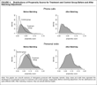
Figure 2 further compares the similarity of the two groups by examining the distributions of the estimated propensity score. Since the propensity score is a scalar summary of all observed covariates, successful matching should produce a matched control group whose propensity score distribution is similar to that of the treatment group. While the distributions of the treatment group (indicated by the gray density) and control-group individuals (indicated by the solid line) are substantially different before matching, they are almost identical after matching.
Distributions of Propensity Scores for Treatment and Control Group Before and After Matching Adjustment
Finally, the same test as shown in Table 6 can be applied to the matched sample. I use the same logistic regression to predict the receipt of each treatment in the sample that combines those who received the treatment with a group of compliers selected by matching. If matching is successful, the model should not predict the receipt of any particular treatment well. The results show that after matching, the model no longer predicts the receipt of treatments. Indeed, using the original data, the p-values for phone calls, personal visits, and postcard mailings are 0.63, 0.67, and 0.65, respectively. For the revised data, the results are 0.84, 0.88, and 0.99. The large p-values contrast with the results in Table 6, confirming that the matched sample balances the covariates between the treatment and the control groups.
The effectiveness of matching illustrates an important advantage of randomized field experiments. In many observational studies, it is often difficult to conduct matching adjustment because the treatment group is too different from the control group. For such cases, even the propensity score may prove inadequate. In field experiments, such problems are less likely because the control group tends to be a representative sample of the relevant population. Despite the randomization problems for phone calls, Gerber and Green's study produced treatment assignment and large control groups for which propensity score matching can effectively balance all covariates.
GET-OUT-THE-VOTE CALLS INCREASE TURNOUT
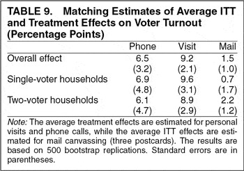
After matching with the estimated propensity score, I calculate the average treatment effects of phone calls and personal canvassing as well as the average ITT effects of mailings (three postcards). Table 9 presents the matching estimates for revised data. The results based on the original data are similar.22
The results for the original data are as follows: 7.1% (3.2) for phone calls, 8.5% (2.1) for visits, and 2.2% (1.1) for postcards, where standard errors are in parentheses.
The results show that get-out-the-vote calls
increase turnout by a little more than six percentage points on average (with a standard error of 3 percentage points), reversing the negative finding reported in Gerber and Green (
2000). While it may not appear as effective as personal visits, telephone canvassing offers a significant alternative mobilization strategy. The matching estimate for personal visits is significantly smaller than the corrected IV estimate. The estimated ITT effect of sending three postcards is about two percentage points. Mailing appears to be especially effective for two person households, suggesting that along with phone calls, mail canvassing may represent another cost-effective mobilization strategy.
Although the overall effect of postcards may appear to be smaller than that of phone calls and visits, such a simple comparison is misleading. While the ITT effect of postcards is estimated for the entire treatment assignment group, the treatment effects of the subgroup of compliers are estimated for the other canvassing methods. In particular, it is possible that postcards may be as effective for compliers as phone calls and visits are for this subgroup. Unless we have the information about who actually read postcards, it is difficult to identify the treatment effect of postcards for compliers.
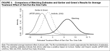
Figure 3 compares the matching estimates with the original results reported in Gerber and Green (2000) as well as the estimates posted on their Web site (see footnote 4). (When analyzing the revised data, Gerber and Green incorrectly identify their treatment and control groups. Thus, their estimates differ from the corrected IV estimates reported in Table 5, which are based on the actual treatment assignment and control groups.) The conclusions one would draw from two statistical methods are clearly different. Matching shows that get-out-the-vote calls increase turnout, whereas Gerber and Green's IV analysis indicates that such calls may discourage voters from casting their ballots. Although Gerber and Green's Web site results are somewhat closer to my matching estimates, the difference shows that the data correction alone is not sufficient to fix all the problems that have occurred when implementing their field experiment.
Comparison of Matching Estimates and Gerber and Green'sResults for Average Treatment Effect of Get-Out-the-Vote Calls
The positive finding about telephone canvassing agrees with the results of another experimental study recently conducted in a different setting by the same authors as well as the earlier experimental results (e.g., Adams and Smith 1980, Eldersveld 1956, and Miller, Bositis, and Baer 1981). In their recent study, Green and Gerber (2001, 2) conclude that “phone canvassing increased turnout by an average of 5 percentage-points. This finding, based on six experiments involving nearly 10,000 people, is statistically significant.”23
These findings were given to me after I sent Don Green the initial version of this article.
Given that making a phone call costs much less than visiting a home, get-out-the-vote calls may be the most cost-effective mobilization strategy.
Sensitivity Analysis
I conduct two kinds of sensitivity analysis. First, I investigate how the matching estimates differ between the two types of households. The instability of IV estimates for phone calls in the original data was apparent from the discrepancy between the large negative effect for single-voter households and the moderately positive effect for two-voter households. In contrast, the estimates based on matching show smaller gaps between the treatment effects for the two types of households.
I also perform one-to-one matching to examine whether it produces different estimates. One-to-one matching is not as efficient as one-to-many matching because a smaller subset of the data is used. However, it may be less biased since many of the selected control units can be exactly matched. If the results based on one-to-many matching are significantly different from those of one-to-one matching, therefore, we may conclude that the former suffers from a large bias.24
I report the results for matching without replacement, but the sensitivity analysis using matching with replacement produced similar results.
In the case of Gerber and Green's data, one-to-one matching gives similar results. In particular, get-out-the-vote calls increase turnout by five and six percentage points on average, respectively, for the original and the revised data. Together with the model specification tests of the previous section, these sensitivity analyses indicate that there is minimal bias in the matching estimates reported in
Table 9.
CONCLUDING REMARKS
Although Gerber and Green correctly argue that field experiments have many advantages over observational studies, they are incorrect to claim that field experiments only require “rudimentary data analysis.” Rather, statistical methods are essential for the analysis of field experiments. Unlike laboratory experiments, field experiments are performed in real world settings. This tremendous advantage of field experiments is, however, accompanied by complications that commonly arise in the real world. While some of these complications can be avoided by a better experimental design and more careful implementation, other problems will normally need to be addressed when conducting the data analysis.
The approach recommended in this article detected the implementation errors of Gerber and Green's experiment. In light of the fact that even this prominent field experiment encountered such problems, it is advisable to apply comprehensive diagnostic analysis such as the methods suggested in this article to all data generated by field experiments. More than 60 years ago, Ronald A. Fisher (1938), who introduced the concept of randomized experiments, stated, “To call in the statistician after the experiment is done may be no more than asking him to perform a postmortem examination: he may be able to say what the experiment died of.” Since then, the field of statistics has made methodological advancements for the analysis of quasi-experimental and non-experimental data. These statistical methods can not only find the problems, but also make necessary adjustments for flawed implementation of a field experiment.
The reanalysis of Gerber and Green's field experiment shows that get-out-the-vote calls increase turnout rather than decrease it. Along with phone calls, postcards also appear to mobilize voters at relatively low cost. After their analysis, Gerber and Green (2000, 662) reached the rather pessimistic conclusion that “The question is whether the long-term decay of civic and political organizations has reached such a point that our society no longer has the infrastructure to conduct face-to-face canvassing on a large scale.” In contrast, my findings allow greater optimism for how to reinvigorate democracy. A simple phone call or postcard can make a difference.
Gerber and Green's study was one of the first large-scale field experiments conducted in the discipline in more than half a century. As more experience with field experiments accumulates, political scientists will learn how to use this promising methodology even more effectively. Nonetheless, there will always be unforeseen complications in the field. The real world is a messy place, and only with statistical methods continuously adapted to the problem at hand are we able to make valid causal inferences.
For easy-to-use software to implement various matching methods including the one used in this article, see Ho, Imai, King, and Stuart (2004) and the accompanying software MatchIt available at http://GKing.Harvard.Edu/MatchIt.
This article was written when the author was a graduate student in the Department of Government at Harvard University, and it is based upon a chapter of his Ph.D. dissertation (Imai 2003). The final version of the manuscript of this article was accepted for publication in August 2003. I thank Don Green for making his data available and answering many follow-up questions. I am indebted to Jim Alt, Gary King, David van Dyk, and Don Rubin for their guidance. I am also grateful for comments from Jason Barabas, Barry Barden, Larry Bartels, Paul Beck, James Fowler, Shigeo Hirano, Dan Ho, Alison Post, and seminar participants at Harvard, Ohio State, Princeton, Stanford, U.C. Berkeley, U.C. Davis, University of Washington, and Washington University, St. Louis. An earlier version of this article, entitled “The Importance of Statistical Methodology for Analyzing Data from Field Experimentation,” was presented at the Annual Meeting of Political Methodology, Seattle, WA, July 2002. Finally, I thank the editor and three anonymous referees for helpful suggestions.






Comments
No Comments have been published for this article.