1. Introduction
Rayleigh–Bénard (RB) convection, a fluid layer heated from below and cooled from above, is a simple yet widely investigated model to study the complex physics behind natural convection (Ahlers, Grossmann & Lohse Reference Ahlers, Grossmann and Lohse2009; Lohse & Xia Reference Lohse and Xia2010; Chillà & Schumacher Reference Chillà and Schumacher2012; Sun & Zhou Reference Sun and Zhou2014; Shishkina Reference Shishkina2021). Many previous studies on RB convection have focused on how the heat transport efficiency and turbulent intensity depend on the control parameters – which are the Rayleigh number, the Prandtl number, and the geometry of the container – particularly on their scaling relationships (Ahlers et al. Reference Ahlers, Grossmann and Lohse2009). Apart from that, the fascinating dynamics of large-scale circulation (LSC), such as its cessations and reversals, have also been investigated extensively over the past few decades (Benzi Reference Benzi2005; Brown & Ahlers Reference Brown and Ahlers2007, Reference Brown and Ahlers2008; Sugiyama et al. Reference Sugiyama, Ni, Stevens, Chan, Zhou, Xi, Sun, Grossmann, Xia and Lohse2010; Assaf, Angheluta & Goldenfeld Reference Assaf, Angheluta and Goldenfeld2011; Petschel et al. Reference Petschel, Wilczek, Breuer, Friedrich and Hansen2011; Vasiliev & Frick Reference Vasiliev and Frick2011; Wagner & Shishkina Reference Wagner and Shishkina2013; Ni, Huang & Xia Reference Ni, Huang and Xia2015; Wang et al. Reference Wang, Xia, Wang, Sun, Zhou and Wan2018a; Zhang et al. Reference Zhang, Xia, Zhou and Chen2020, Reference Zhang, Chen, Xia, Xi, Zhou and Chen2021). In general, there are two categories of flow reversals classified by their distinct physical mechanisms. In the cylindrical geometry, the reversals can be caused by azimuthal rotations of the vertically circulating plane of the LSC due to the azimuthal symmetry. The reversals can also be led by cessation of the circulating flow (Cioni, Ciliberto & Sommeria Reference Cioni, Ciliberto and Sommeria1997; Brown, Nikolaenko & Ahlers Reference Brown, Nikolaenko and Ahlers2005; Sun, Xi & Xia Reference Sun, Xi and Xia2005; Xi, Zhou & Xia Reference Xi, Zhou and Xia2006). Note that the second type of reversal can take place in both three-dimensional (3-D) and two-dimensional (2-D) geometries (Tsuji et al. Reference Tsuji, Mizuno, Mashiko and Sano2005; Xi & Xia Reference Xi and Xia2007).
In spite of the complicated 3-D flow dynamics such as the torsional and sloshing motions of the LSC (Funfshilling, Brown & Ahlers Reference Funfshilling, Brown and Ahlers2008; Brown & Ahlers Reference Brown and Ahlers2009; Xi et al. Reference Xi, Zhou, Zhou, Chan and Xia2009; Zhou et al. Reference Zhou, Xi, Zhou, Sun and Xia2009), a (quasi-)2-D set-up was often chosen as a particular configuration to study flow reversals that can minimize the 3-D flow effects. In (quasi-)2-D, the geometry will limit the azimuthal position of the LSC plane, and with the removal of the complicated 3-D dynamics, some essential features of the reversal dynamics may be revealed (Ni et al. Reference Ni, Huang and Xia2015). Motivated by this, Sugiyama et al. (Reference Sugiyama, Ni, Stevens, Chan, Zhou, Xi, Sun, Grossmann, Xia and Lohse2010) explored, both numerically and experimentally, a wide parameter space of flow reversals in 2-D and quasi-2-D square boxes.They found that the growth of corner rolls plays an essential role in the reversal process and then analysed the dynamics of reversals based on the energy balance of corner rolls, such that we focus mainly on the reversal led by corner rolls. A Fourier-based approach has also been adopted to quantify the strength of the flow rolls and their time evolution (Chandra & Verma Reference Chandra and Verma2011). This quantitative approach also helps to unveil the role of vortex reconnection in leading to the flow reversal. Besides these, a couple of theoretical approaches have also been proposed to describe the physical mechanisms of the chaotic flow reversals (Sreenivasan, Bershadskii & Niemela Reference Sreenivasan, Bershadskii and Niemela2002; Araujo, Grossmann & Lohse Reference Araujo, Grossmann and Lohse2005). Other recent works on flow reversals can be found in Ni et al. (Reference Ni, Huang and Xia2015), Podvin & Sergent (Reference Podvin and Sergent2015), Wang et al. (Reference Wang, Lai, Song and Tong2018b), Chen et al. (Reference Chen, Huang, Xia and Xi2019), Chen, Wang & Xi (Reference Chen, Wang and Xi2020), Zhang et al. (Reference Zhang, Xia, Zhou and Chen2020, Reference Zhang, Chen, Xia, Xi, Zhou and Chen2021) and Xu, Chen & Xi (Reference Xu, Chen and Xi2021).
In recent studies of LSC reversals, how the boundary conditions, geometries of convection cells and fluid properties influence the reversal behaviours is examined. Huang et al. (Reference Huang, Wang, Xi and Xia2015) reported that the reversal frequency could be reduced when a fixed heat flux boundary condition is applied to the bottom plate of the cell. Zhang et al. (Reference Zhang, Xia, Zhou and Chen2020, Reference Zhang, Chen, Xia, Xi, Zhou and Chen2021) found that reversals of the LSC in 2-D RB convection can be suppressed or enhanced by imposing local constant-temperature control on sidewalls, which offers a new way to control the reversals. Xia et al. (Reference Xia, Wan, Liu, Wang and Sun2016) considered the non-Oberbeck–Boussinesq effects and found a different mechanism for the growth-induced reversals of corner-flow rolls. Wang et al. (Reference Wang, Xia, Wang, Sun, Zhou and Wan2018a) found that the tilting of the cell tends to suppress flow reversals for a convection cell of aspect ratio 1, but reversals characterized by two main rolls are promoted by tilting for a larger aspect ratio. Wang et al. (Reference Wang, Lai, Song and Tong2018b) and Chen et al. (Reference Chen, Wang and Xi2020) reported a comparative experimental study of flow reversals of the LSC in an upright cylindrical cell or a cornerless cell. Despite the absence of corner rolls, LSC reversals can still happen, and the reversal frequency decreases with  $Ra$. Other methods of controlling the flow dynamics are also introduced, such as adding particles (Liu & Zhang Reference Liu and Zhang2008), imposing magnetic fields (Sterl, Li & Zhong Reference Sterl, Li and Zhong2016), using wall roughness (Jiang et al. Reference Jiang, Zhu, Mathai, Verzicco, Lohse and Sun2018; Emran & Shishkina Reference Emran and Shishkina2020), and so on (see e.g. Sun et al. Reference Sun, Xi and Xia2005; Brown & Ahlers Reference Brown and Ahlers2008; Verma, Ambhire & Pandey Reference Verma, Ambhire and Pandey2015; Wang et al. Reference Wang, Xu, Xia, Wan and Sun2017).
In this paper, we report a numerical study on how the spatially harmonic heating of the bottom plate influences the flow reversals in thermal convection. In fact, turbulent convection driven by a non-uniform temperature distribution is ubiquitous in nature and many industrial applications, with examples including atmospheric circulation subjected to spatially non-uniform heating on the Earth's surface, and the convective flows induced by spatially distributed heat sources in devices like computer chips (Freund, Pesch & Zimmermann Reference Freund, Pesch and Zimmermann2011; Mau, Hagberg & Meron Reference Mau, Hagberg and Meron2012; Weiss, Seiden & Bodenschatz Reference Weiss, Seiden and Bodenschatz2012; Jovanović, Nikodijević & Nikodijević Reference Jovanović, Nikodijević and Nikodijević2015; Nepomnyashchy & Simanovskii Reference Nepomnyashchy and Simanovskii2018). In addition, it is known that non-uniform heating induces unstable vertical and horizontal pressure gradients, giving rise to horizontal convection regardless of the heating intensity (Hughes & Griffiths Reference Hughes and Griffiths2008; Abtahi & Floryan Reference Abtahi and Floryan2017; Yang et al. Reference Yang, Wang, Wu, Lu and Zhou2021b). This may affect the global responses of turbulent flows and offer the possibility of controlling the pattern of convection rolls. Here, we apply direct numerical simulation of 2-D convection with spatially heating modulation. We explore a wide parameter space and find an extended parameter regime where flow reversals can be suppressed. We show that the proposed set-ups can suppress the flow reversals, depending on the wavenumber of the spatial modulation, and the underlying mechanism has also been discussed.
The remainder of the paper is organized as follows. The numerical set-ups are introduced briefly in § 2. Then the results are shown in § 3. In § 3.1, we analyse the effects of spatial modulation on the flow reversal frequency. In § 3.2, we investigate the behaviours of flow reversals due to modulation by examining the size of corner-flow rolls. In § 3.3, we adopt the Fourier mode decomposition method to distinguish clearly the difference between the unmodulated and modulated reversals. In § 3.4, we rationalize the cause of corner-roll suppression. In § 3.5, we introduce the concept of horizontal convection led by non-uniform heating to describe how the reversal frequency depends on wavenumber and amplitude. Finally, a summary is presented in § 4.
2. Numerical set-ups
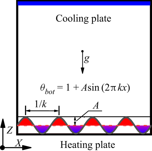
In the present study, we consider 2-D RB convection in a square enclosure. Spatially harmonic heating from below is applied to control flow reversals of the LSC, as shown in figure 1. The non-dimensional governing equations under the Boussinesq approximations read
 $$\begin{gather} \boldsymbol{\nabla} \boldsymbol{\cdot} \boldsymbol{u} = 0, \end{gather}$$
 $$\begin{gather}\partial_t \boldsymbol{u}+(\boldsymbol{u}\boldsymbol{\cdot} \boldsymbol{\nabla})\boldsymbol{u}={-}\boldsymbol{\nabla} p+ \left(\frac{Ra}{Pr}\right)^{{-}1/2}\nabla^2\boldsymbol{u}+\theta \boldsymbol{e}_z, \end{gather}$$
 $$\begin{gather}\partial_t \theta + (\boldsymbol{u}\boldsymbol{\cdot}\boldsymbol{\nabla}) \theta=(Ra\,Pr)^{{-}1/2}\,\nabla^2\theta, \end{gather}$$
where  $t$ is the dimensionless time scaled by the free-fall time
 $\sqrt {H/(\alpha g \varDelta )}$,
 $\boldsymbol {u} = (u\boldsymbol {e}_x, w\boldsymbol {e}_z)$ is the fluid velocity scaled by the free-fall velocity
 $\sqrt {\alpha g\,\varDelta H}$,
 $\theta$ is the temperature scaled by the mean temperature difference
 $\varDelta$ between the two plates (using the spatial mean at the bottom plate), and
 $\boldsymbol {e}_x$ and
 $\boldsymbol {e}_z$ are, respectively, the horizontal and vertical unit vectors. All length scales are normalized by the cell height
 $H$. In the governing equations (2.1)–(2.3), there are two control parameters for the RB system: the Rayleigh number
 $Ra$ and the Prandtl number
 $Pr$. They are defined as
 \begin{equation} Ra = \frac{\alpha g\,\varDelta H^3}{\nu \kappa}, \quad Pr = \frac{\nu}{\kappa}, \end{equation}
where  $\alpha$ is the thermal expansion coefficient,
 $g$ is the gravitational acceleration,
 $\nu$ is the kinematic viscosity, and
 $\kappa$ is the thermal diffusivity of the working fluid. In the spatially modulated RB system, no-slip velocity boundary conditions are used on all the walls. The adiabatic condition is used on the two sidewalls, and constant temperature
 $\theta _{top} = 0$ is applied on the top plate, and a sinusoidally distributed heating on the bottom plate:
 \begin{equation} \theta_{bot}(x) = 1 + A \sin(2{\rm \pi} k x), \end{equation}
where  $A$ is the dimensionless modulation amplitude of temperature, and
 $k$ the dimensionless modulation wavenumber.
Sketch of the convection cell under spatially harmonic heating from below,  $\theta _{bot} = 1 + A \sin (2{\rm \pi} k x)$, with the associated coordinate system. Here,
 $A$ is the dimensionless modulation temperature amplitude, and
 $k$ is the dimensionless modulation wavenumber.

In this study, we performed direct numerical simulations using the spectral element code Nek5000, which has been well validated (Chandra & Verma Reference Chandra and Verma2013; Pandey, Scheel & Schumacher Reference Pandey, Scheel and Schumacher2018; Wang, Zhou & Sun Reference Wang, Zhou and Sun2020). We fix  $Ra = 10^8$,
 $Pr = 4.38$, and focus on the influence of the modulation wavenumber
 $k$ and amplitude
 $A$ on the flow reversals in turbulent RB convection. In our numerical simulations, the uniform grid is adopted horizontally, while the grid is stretched vertically to guarantee that more grid points are located near the top and bottom walls to resolve accurately the boundary layers (Shishkina et al. Reference Shishkina, Stevens, Grossmann and Lohse2010). For each run, the grid size is chosen to resolve adequately both the Kolmogorov length scale for the velocity field
 $\boldsymbol {u}$ and the Batchelor length scale for the temperature field
 $\theta$. The Kolmogorov scale is estimated by the global criterion
 $\eta =(\nu ^3/\varepsilon )^{1/4}=H\,Pr^{1/2}/[Ra\,(Nu-1)]^{1/4}$, and the Batchelor scale by
 $\eta _{B}=\eta \,Pr^{-1/2}$ (Zhang, Zhou & Sun Reference Zhang, Zhou and Sun2017; Tsai et al. Reference Tsai, Hussam, King and Sheard2020). More than
 $25$ quadrature points are nested within the boundary layers in the vertical direction, and at least
 $15$ quadrature points are within the modulation wavelength in the horizontal direction for large wavenumbers. In detail, the order of the Legendre polynomials is fixed at
 $8$, and the number of spectral elements increases from
 $50 \times 50$ at
 $k = 2$ to
 $160 \times 50$ at
 $k = 80$. Also, a grid independence test has been conducted to ensure that the same final conclusion has been obtained when the grid size is halved. The time step adopted is set to be small enough to guarantee the numerical stability and resolve the Kolmogorov time scale of turbulent fluctuations. For each case, when the flow reaches the statistical steady state, we evaluate the statistics over a time interval of more than 10 000 free-fall time units to examine the flow reversal behaviours.
3. Results and discussion
3.1. Reversal frequency versus wavenumbers
Flow reversals can be identified through different approaches, such as the temperature contrast between the left and right walls (Ni et al. Reference Ni, Huang and Xia2015; Chen et al. Reference Chen, Huang, Xia and Xi2019), and the sign change of angular momentum (Sugiyama et al. Reference Sugiyama, Ni, Stevens, Chan, Zhou, Xi, Sun, Grossmann, Xia and Lohse2010; Wang et al. Reference Wang, Xia, Wang, Sun, Zhou and Wan2018a; Zhang et al. Reference Zhang, Xia, Zhou and Chen2020). Here, we use the latter approach, with the global angular momentum being defined as (Sugiyama et al. Reference Sugiyama, Ni, Stevens, Chan, Zhou, Xi, Sun, Grossmann, Xia and Lohse2010)
 \begin{equation} L(t) = \langle (x-0.5)w-(z-0.5)u \rangle_{A}, \end{equation}
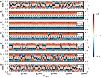
where  $\langle \cdot \rangle _{A}$ represents the average over the entire 2-D plane. In figure 2, we plot the time series of
 $L(t)$ and the vertical slice of the horizontal velocity
 $u$ at mid-width (
 $x=0.5$) for different wavenumbers
 $k= 4$, 15, 25, 30, 40, 80. In the standard RB convection without spatial modulation, frequent flow reversals are observed as shown in figure 2(a), namely
 $L(t)$ changing its sign frequently. However, when we apply spatially harmonic heating on the bottom plate, the frequency of flow reversal can reduce drastically. In cases
 $k=4$ and
 $k=15$, one has
 $L(t)<0$ over the whole examined time period, indicating a successful elimination of the flow reversal. As the wavenumber
 $k$ increases, there exists an intermediate regime with a significant inhibition of flow reversals, in which the flow reversal still happens, but its frequency is less than that of the standard RB convection without modulation. With
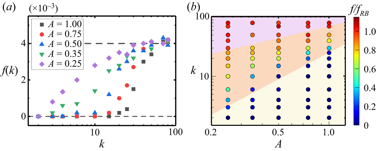
 $k$ increasing further, the flow reversal frequency becomes close to that of the standard RB convection. This trend is also observed at small amplitudes
 $A$, as shown in figure 3(a), where we plot the measured reversal frequency
 $f$ as a function of wavenumber
 $k$ for various modulation amplitudes
 $A$. Here, the reversal frequency
 $f$ is defined as the averaged number of flow reversals per unit time. Moreover, it is found that the intermediate regime shifts towards larger
 $k$ with increasing
 $A$, suggesting that the rise of amplitude
 $A$ promotes the stabilization of LSC and in turn enhances the inhibition ability of the reversal.
Time series of the angular momentum  $L(t)$ (black curves) and the the vertical slice of horizontal velocity
 $u$ at mid-width (
 $x=0.5$) at
 $Ra=10^8$,
 $Pr=4.38$, for (a) standard RB convection, and under spatial temperature modulation with different modulation wavenumbers at
 $A=1$: (b)
 $k=4$, (c)
 $k=15$, (d)
 $k=25$, (e)
 $k=30$, ( f)
 $k=40$, (g)
 $k=80$.

(a) Reversal frequency  $f$ via heating wavenumber
 $k$ for various modulation temperature amplitude
 $A$. (b) Phase diagram in the
 $A$–
 $k$ plane with the contour of relative values of
 $f/f_{{RB}}$, where
 $f_{{RB}}$ denotes the reversal frequency of standard RB convection without modulation.

Figure 3(b) shows the phase diagram in the plane of control parameters  $k$ and
 $A$ for fixed
 $Ra=10^8$ and
 $Pr=4.38$, in which the colour of the symbol represents the value of normalized reversal frequency
 $f/f_{{RB}}$, where
 $f_{{RB}}$ is the reversal frequency of standard RB convection without modulation. According to the value of
 $f/f_{{RB}}$, the modulation of flow reversals by the spatially harmonic heating can be categorized roughly into three regimes, marked by different background colours in figure 3(b): the reversal-elimination regime (yellow-shaded area) identified by
 $f_{k}\approx f_{bound}$ (where
 $\lvert f_k / f_{bound}-1\rvert \leqslant c_\epsilon$, with the threshold value
 $c_\epsilon = 0.05$); the reversal-inhibition regime (orange-shaded area) identified by
 $f_{bound}\leqslant f_{k}\leqslant f_{RB}$; and the RB-like regime (pink-shaded area) identified by
 $f_{k}\approx f_{RB}$ (where
 $\lvert f_k / f_{RB}-1\mid \leqslant c_\epsilon$). It should be noted that the reversal frequency is calculated from the simulation duration of at least 10 000 free-fall time units to examine large-scale flow reversals. If the reversal does not occur during the whole duration, then the reversal frequency is set to be its upper bound, i.e.
 $f_{bound}=1/t_{total}$, with
 $t_{total}$ being the total duration of statistics.
3.2. Suppression of corner rolls
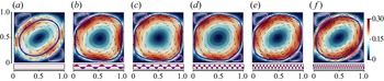
To understand the physical mechanism of the three regimes, we first examine whether the change of the reversal frequency is related to the strength of the corner roll. According to previous results (Sugiyama et al. Reference Sugiyama, Ni, Stevens, Chan, Zhou, Xi, Sun, Grossmann, Xia and Lohse2010; Chen et al. Reference Chen, Huang, Xia and Xi2019), the dynamics of corner-flow rolls plays an important role in the flow reversal process. The growth of corner rolls destabilizes the LSC, and therefore increases the occurrences of flow reversal. This prompts us to investigate directly the state of corner rolls for the cases with and without spatial modulation. Figure 4 shows typical contours of the velocity magnitude at five different  $k$ values for
 $A=1$, which is conditionally averaged over the duration with
 $L(t)<0$. To better compare the shape and size of rolls, we plot the circulation path that passes through the points having maximum local velocity in the time-averaged velocity field, which is also known as the ‘particle path’ (Sun & Xia Reference Sun and Xia2005). It is seen that for the standard RB case (figure 4a), the flow consists of a main roll of a tilted elliptic shape and two corner rolls (lower right and upper left) diagonally opposite to each other. However, the flow structure becomes different when the spatial temperature modulation is applied. It is observed in figure 4 that the spatial modulation with sufficiently small
 $k$ is able to suppress or even eliminate the corner roll (lower right) near the bottom plate. Towards the larger
 $k$ values, the size of the corner roll grows with the increasing modulation wavenumber
 $k$ and tends to the size in the standard RB convection over the limit of high
 $k$.
Contours of the time-averaged velocity magnitude (colour) during a period  $L(t)<0$ in (a) the standard RB convection, and for five different wavenumbers at
 $A=1$: (b)
 $k=4$, (c)
 $k=6$, (d)
 $k=10$, (e)
 $k=15$, ( f)
 $k=25$. The circulation path (blue and pink curves) is defined as the streamline passing through the position with the maximum local speed in the time-averaged flow field.

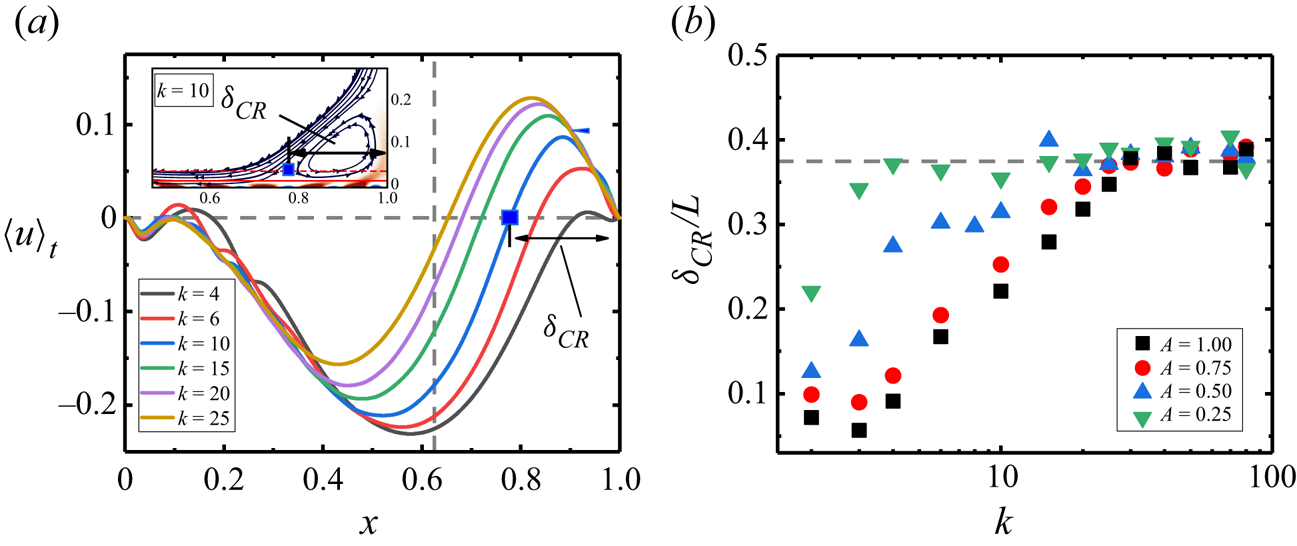
To gain a quantitative understanding of the growth of corner rolls, we define the size of the lower-right corner-flow roll  $\delta _{{CR}}$ (see figure 5a) using the horizontal distance from the sidewall to the zero-crossing or stagnation point of the horizontal velocity near the bottom plate at the edge of the viscous boundary layer (Shishkina, Wagner & Horn Reference Shishkina, Wagner and Horn2014). We evaluate the size of the corner rolls
 $\delta _{{CR}}$ for various modulation amplitudes
 $A$ as shown in figure 5(b). It is seen that for small wavenumbers, the corner roll grows monotonically with
 $k$, whereas for sufficiently large wavenumbers,
 $\delta _{{CR}}$ is not sensitive to the modulation wavenumbers, and the value of
 $\delta _{{CR}}$ is close to that in the standard RB case without modulation (marked by the horizontal dashed line in figure 5b). It should be noted that once the sizes of both corner rolls fluctuate to about
 $0.5H$, the main convection roll may break up, and a new roll circulating in the opposite direction will be formed via the connection of corner rolls (Sugiyama et al. Reference Sugiyama, Ni, Stevens, Chan, Zhou, Xi, Sun, Grossmann, Xia and Lohse2010; Chandra & Verma Reference Chandra and Verma2013).
(a) Profiles of time-averaged horizontal velocity  $u$ at the edge of the viscous boundary layer for different wavenumbers
 $k$ at
 $A=1$. The blue square marks the zero-crossing point for the
 $k=10$ case, and illustrates how
 $\delta _{{CR}}$ is determined. The vertical dashed line marks the zero-crossing position of the lower-right corner roll obtained in the standard RB case without modulation. Inset shows the streamlines of the time-averaged velocity field at the lower-right corner of the cell for the
 $k=10$ case. The red dashed line indicates the edge of the viscous boundary layer. (b) Size of the corner roll
 $\delta _{{CR}}$ as a function of the wavenumber
 $k$ for various modulation temperature amplitudes
 $A$. The horizontal dashed line marks the size of the lower-right corner roll obtained in the standard RB case without modulation.

3.3. Mode analysis
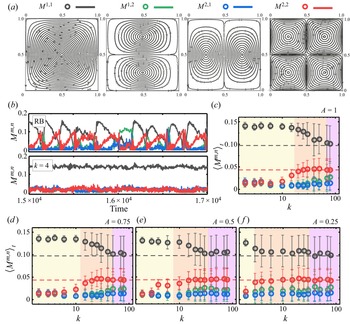
To compare the dynamics of flows in different regimes, we quantify the flow structures with the help of the Fourier mode decomposition method. This method is suitable for 2-D or quasi-2-D convection patterns, and has been adopted in many previous studies on the flow topology of RB convection (Chandra & Verma Reference Chandra and Verma2013; Wagner & Shishkina Reference Wagner and Shishkina2013; Horstmann, Schiepel & Wagner Reference Horstmann, Schiepel and Wagner2018; Chen et al. Reference Chen, Huang, Xia and Xi2019; Wan et al. Reference Wan, Wei, Verzicco, Lohse, Ahlers and Stevens2019). Briefly, each instantaneous velocity field  $(u, w)$ is projected onto the Fourier modes, given as
 $$\begin{gather} \hat{u}^{m,n} = 2\sin(m{\rm \pi} x)\cos(n{\rm \pi} z), \end{gather}$$
 $$\begin{gather}\hat{w}^{m,n} ={-}2\cos(m{\rm \pi} x)\sin(n{\rm \pi} z), \end{gather}$$
where  $m = 1, 2$ and
 $n = 1, 2$ are considered. It corresponds to a flow structure with
 $m$ rolls in the
 $x$ direction, and
 $n$ rolls in the
 $z$ direction (see figure 6a). The velocity field can be recovered by
 $$\begin{gather} u(x,z,t) = \sum_{m,n} A^{m,n}_{x}(t)\,\hat{u}^{m,n}, \end{gather}$$
 $$\begin{gather}w(x,z,t) = \sum_{m,n} A^{m,n}_{z}(t)\,\hat{w}^{m,n}. \end{gather}$$
The corresponding time series  $A^{m,n}_x(t)$ and
 $A^{m,n}_z(t)$ can be obtained by projecting each individual snapshot onto the Fourier basis
 $$\begin{gather} A^{m,n}_{x}(t) = \int_{0}^{x_{max}}\int_{0}^{z_{max}}u(x,z,t)\,\hat{u}^{m,n}\,\mathrm{d} x\,\mathrm{d}z, \end{gather}$$
 $$\begin{gather}A^{m,n}_{z}(t) =\int_{0}^{x_{max}}\int_{0}^{z_{max}}w(x,z,t)\,\hat{w}^{m,n}\,\mathrm{d} x\,\mathrm{d}z. \end{gather}$$
Then the instantaneous amplitude of each mode  $M^{m,n}(t)$ representing the mode contribution can be evaluated by
 $M^{m,n}(t)=\sqrt {A^{m,n}_x(t)^2+A^{m,n}_z(t)^2}$. Here, we focus on the first four modes,
 $M^{1,1}$,
 $M^{1,2}$,
 $M^{2,1}$,
 $M^{2,2}$, which are usually the dominant ones (Chandra & Verma Reference Chandra and Verma2011, Reference Chandra and Verma2013; Wagner & Shishkina Reference Wagner and Shishkina2013; Chong et al. Reference Chong, Wagner, Kaczorowski, Shishkina and Xia2018; Chen et al. Reference Chen, Huang, Xia and Xi2019, Reference Chen, Wang and Xi2020; Xu et al. Reference Xu, Chen and Xi2021). The corresponding global flow structures are drawn in figure 6(a) to give an impression. Then in this subsection we analyse the
 $M^{m,n}$ by projecting each snapshot onto four distinct modes, and evaluate their time series, time averages and temporal fluctuations (represented by standard deviations).
(a) Illustration of the first four dominant Fourier mode structures. (b) Time series of  $M^{m,n}$ in the cells with
 $k=4$ and without spatial modulation. (c–f) Time-averaged contribution of each mode
 $M^{m,n}$ as a function of
 $k$ for various modulation amplitudes: (c)
 $A=1$, (d)
 $A=0.75$, (e)
 $A=0.5$, ( f)
 $A=0.25$. The error bars indicate the standard deviations. Three flow regimes (see also figure 3b) are identified and indicated by different colours: the reversal-elimination regime (yellow), the reversal-inhibition regime (orange), and the RB-like regime (pink).

Figure 6(b) shows the time series of  $M^{m,n}$ in the cells with
 $k=4$ and without spatial modulation. In the standard RB convection, as the flow reversal occurs frequently, the value of
 $M^{m,n}$ exhibits large temporal variations with the interchange of mode dominance. During the reversals, the mode
 $M^{1,1}$ reduces to almost zero, whereas
 $M^{2,2}$ shows a spike that agrees with previous studies (Chandra & Verma Reference Chandra and Verma2011). For the
 $k=4$ case, the single-roll mode
 $M^{1,1}$ always dominates the flow, and the magnitudes of all other modes remain at very small values, which again confirms the largely suppressed corner rolls.
To compare the strength of each mode  $M^{m,n}$ for the different wavenumbers, we calculate the time-averaged contribution of each mode (
 $M^{1,1}$,
 $M^{1,2}$,
 $M^{2,1}$,
 $M^{2,2}$) as a function of modulation wavenumbers
 $k$ in figures 6(c–f), where the error bars show the corresponding standard deviations that can be used to quantify the fluctuations of
 $M^{m,n}$. Three different colours in figure 6(c–f) correspond to the three regimes identified in figure 3(b).
Within the reversal-elimination regime (yellow), only the single-roll mode ( $M^{1,1}$) contains a considerable contribution, while all three other modes stay at a small value. Compared with the standard RB convection, single-roll mode
 $M^{1,1}$ (LSC) enhances, and the
 $M^{2,2}$ (corner rolls) are suppressed. Moreover, there is small fluctuation of each
 $M^{m,n}$, suggesting the robustness of the single-roll mode.
Next, in the reversal-inhibition regime (orange),  $M^{1,1}$ is still the dominant mode. Only the contribution of the single-roll mode is of great significance, which strengthens the LSC stability, and in turn drastically reduces the frequency of flow reversal. However, with increasing
 $k$, the single-roll mode becomes weaker, as is evident from the smaller
 $M^{1,1}$, and its value is getting close to that without modulation (black dashed line in figures 6(c–f)). Also, a substantial amount of contribution is contained in the mode
 $M^{2,2}$, indicative of dynamically active corner rolls. In the meantime, the fluctuations of each mode start to increase. Accordingly, the reduction in
 $M^{1,1}$ and enhancement in
 $M^{2,2}$ facilitate the flow reversal. With increasing
 $k$, the reversal frequency gradually increases, and becomes close to that of the standard RB convection without modulation.
Finally, in the RB-like regime (pink), the magnitude of all modes becomes insensitive to the change in  $k$, and
 $M^{1,1}$ and
 $M^{2,2}$ are the first and second dominant modes with large fluctuations. For high
 $k$, the accordance of
 $M^{1,1}$ and
 $M^{2,2}$ with the RB case suggests that the reversal frequency nearly equals that of the standard RB convection. Indeed, the difference in the three regimes can be distinguished by the different dominant Fourier modes during reversals via Fourier mode decomposition. Hence through the analysis in figure 6, the flow dynamics of the three regimes are revealed, which supports that the flow essences of the three regimes are different.
3.4. Cause of corner-roll suppression
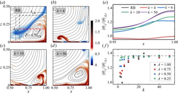
So far, a question remains: how can we understand the suppression of the corner roll by spatial temperature modulation? Sugiyama et al. (Reference Sugiyama, Ni, Stevens, Chan, Zhou, Xi, Sun, Grossmann, Xia and Lohse2010) described the role of the corner flows during the reversal process. Owing to energetic feeding by the detaching plumes from the boundary layers trapped in the corner, the small corner rolls will grow until they reach the half-height, and then they will destroy the main LSC and establish a new LSC in the opposite direction (Sugiyama et al. Reference Sugiyama, Ni, Stevens, Chan, Zhou, Xi, Sun, Grossmann, Xia and Lohse2010; Zhang et al. Reference Zhang, Xia, Zhou and Chen2020, Reference Zhang, Chen, Xia, Xi, Zhou and Chen2021). Here, we inspect closely the behaviour of thermal plumes within the corner-roll region. In figures 7(a–d), we zoom into the lower-right corner-roll region, and show the instantaneous velocity streamlines together with the corresponding temperature fields.
(a–d) Behaviour of thermal plumes within the lower-right corner-roll region. Visualization of instantaneous temperature fields obtained for (a) standard RB convection, and under spatial temperature modulation with different wavenumbers at  $A=1$: (b)
 $k=4$, (c)
 $k= 10$, (d)
 $k=50$. (e) Time-averaged horizontal profiles of temperature obtained at the mid-height of the corner-flow rolls (
 $z=0.5\delta _{{CR}}$) at various
 $k$. ( f) Plot of the peak temperature (obtained at
 $z=0.5\delta _{{CR}}$ and
 $x=1$) as a function of
 $k$ for various
 $A$; the dashed line is the value corresponding to the classical RB convection. Here, the space–time average temperature
 $\langle \theta \rangle _{{A,t}}$ has been used to normalize the measured time-averaged temperature
 $\langle \theta \rangle _{{t}}$.

For the pure RB case shown in figure 7(a), the detached hot plumes are carried by the corner flow and steered to the sidewall. Then these hot plumes move upwards along the sidewall, and they encounter and interact with the confronting cold plumes carried by the main LSC. This flow pattern is the same as observed in previous studies (Sugiyama et al. Reference Sugiyama, Ni, Stevens, Chan, Zhou, Xi, Sun, Grossmann, Xia and Lohse2010; Huang & Zhou Reference Huang and Zhou2013; Zhang et al. Reference Zhang, Zhou and Sun2017, Reference Zhang, Sun, Bao and Zhou2018; Yang et al. Reference Yang, Zhang, Jin, Dong, Wang and Zhou2021a). However, for small  $k$ (e.g.
 $k=10$), the influence of the cold zone can become significant, such that the steered hot plumes lose large amounts of energy content before reaching the adiabatic sidewalls. For instance, the hot plumes are not able to reach the sidewall due to the loss of energy when crossing over the cold phase, as shown in figure 7(c), or even twist the moving direction in the opposite one due to the effect of the cold zone, as shown in figure 7(b). This effect diminishes with increasing
 $k$ since the influence of the cold zone becomes limited in the boundary layers and does not penetrate into the bulk. For instance, at
 $k = 50$, the cold zone is too small to affect the dynamics of thermal plumes, and the corner flow resembles that in the pure RB case, as shown in figure 7(d).
To confirm the picture of losing energy content of the hot plumes, we compare horizontal profiles of temperature obtained at the mid-height of the corner-flow rolls ( $z=0.5\delta _{{CR}}$) shown in figure 7(e). We focus on the peak of temperature profiles at the sidewall in the corner-roll region (
 $\delta _{{CR}} \times \delta _{{CR}}$), which is caused by the plume rising with the corner roll. First, for all
 $k$, the highest temperature locates at the sidewall. As
 $k$ increases, the magnitudes of peaks increase. Then figure 7( f) shows the plot of the peak temperature (obtained at
 $z=0.5\delta _{{CR}}$ and
 $x=1$) as a function of
 $k$ for various amplitudes
 $A$. One can see that there is a significant decrease of
 $\langle \theta \rangle _{{t}}/\langle \theta \rangle _{{A,t}}$ for the spatially harmonic heating cases. This indicates that the regions of the cold phase indeed absorb heat from hot plumes and thus lower their temperature when they reach the sidewall. As a result, this reduces the kinetic energy input for the corner roll brought about by the buoyancy force, and breaks the feeding process of the corner rolls. This results in the locking of the corner roll into a smaller region near the corner, making it harder for a reversal to occur. Note that although the reversal frequency has been largely reduced to a very small value, the LSC reversal may still happen due to the instability of LSC itself, but not via the influence of the corner rolls, when the run lasts long enough (Wang et al. Reference Wang, Lai, Song and Tong2018b; Chen et al. Reference Chen, Wang and Xi2020). For studying the reversal led by LSC instability, and how such instability is influenced by non-uniform heating, experiments should be conducted in the future that are able to capture events with a much longer time scale.
From these results, we conclude that the spatial modulation can affect the corner-roll flow dynamics, i.e. it can suppress successfully and even eliminate the corner roll if  $k$ and
 $A$ are chosen properly. When
 $k$ is very small, the corner rolls are suppressed. The majority of the energy of the flow is in the single-roll mode (
 $M^{1,1}$), and the LSC is very strong. Therefore, the LSC becomes robust, and it is difficult to be interrupted by corner rolls. As the wavenumber
 $k$ increases, the strength of corner rolls increases. The development of corner rolls affects the stability of the LSC, and thus leads to the occurrence of reversals. As
 $k$ increases further, the effects of non-uniform heating are restricted. Therefore, it has little influence on the dynamics of the flows.
3.5. Horizontal convection led by non-uniform heating
From figure 2, for sufficiently low wavenumbers, it is evident that the symmetry breaking induced by spatial modulation suppresses flow reversals for  $A=1$. One sees that the anticlockwise main roll with positive
 $L(t)$ stays for quite a short time before reversing its orientation. This is because for the integer values of
 $k$ adopted in this study, this function is asymmetric when reflected about the vertical centreline of the cavity. This introduces intrinsically a horizontal non-uniformity in the buoyancy supplied through this boundary – horizontal convection. Horizontal convection flows produce a bulk overturning circulation at all finite Rayleigh numbers; this overturning will always rise from the hotter end of a horizontal bottom boundary, and descend at the cooler end (Mullarney, Griffith & Hughes Reference Mullarney, Griffith and Hughes2004; Sheard & King Reference Sheard and King2011; Griffiths, Hughes & Gayen Reference Griffiths, Hughes and Gayen2013; Tsai et al. Reference Tsai, Hussam, King and Sheard2020). Therefore, the spatial modulation may strengthen the clockwise LSC since along the hot and cold plates, the horizontal buoyancy force is in the same direction as the flow velocity of LSC. For the anticlockwise LSC, the hot plumes are more likely to move up to the bottom-left corner roll, and the cold plumes tend to move down to the top-right corner roll. The two corner rolls have more opportunities to grow and trigger a reversal. Thus the anticlockwise LSC is less stable, it is easier to reverse its orientation, and it always stays for a much shorter time, as shown in figure 2.
One way to quantify this asymmetry is to evaluate a temperature ‘moment’ at the bottom boundary. Considering only the fluctuating part of the bottom temperature  $\tilde{\theta}_{bot} = A \sin(2 {\rm \pi}k x)$, this moment can be constructed (with
 $k$ taken as integer) from
 \begin{equation} \int_{0}^{1}x \times \tilde{\theta}_{bot}(x)\,\mathrm{d} x=\int_{0}^{1}Ax\sin(2{\rm \pi} kx)\,\mathrm{d} x={-}\frac{1}{2{\rm \pi}}\left( \frac{A}{k}\right) . \end{equation}
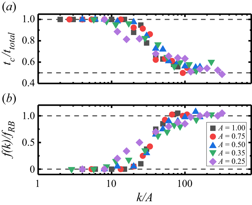
To confirm this proposed physical picture, we measured the percentage of time that the LSC was in the clockwise direction,  $t_c/t_{{total}}$. We replot
 $t_c/t_{{total}}$ and
 $f(k)/f_{{RB}}$ as functions of
 $k/A$ for various values of
 $A$ in figure 8. The figure shows that with
 $k/A$ increasing,
 $t_c/t_{{total}}$ becomes close to 0.5, and the flow reversal frequency becomes close to that of the standard RB convection. We observe that using
 $k/A$ as the parameter, all data display a similar trend. In particular, the data decline to half-maximum at almost the same
 $k/A$. However, one can still see the deviation of the data points for various
 $A$ from close inspection. This suggests that the parameter
 $k/A$ cannot fully explain the onset and settling points of the trends.
The ratios (a)  $t_c/t_{total}$ and (b)
 $f(k)/f_{RB}$ as functions of
 $k/A$, for various modulation temperature amplitudes
 $A$. Here,
 $t_c$ is the time that the LSC was in the clockwise direction.

4. Summary
In summary, we have performed a comprehensive numerical study in 2-D RB convection under spatially harmonic heating. We investigate the events of flow reversals from the perspective of local corner-roll and global flow structures. The LSC reversals can be suppressed using spatial temperature modulation when the modulation wavenumber  $k$ and amplitude
 $A$ are chosen properly. According to the reversal frequency
 $f(A,k)$, three regimes are identified in the phase diagram: the reversal-elimination regime, the reversal-inhibition regime and the RB-like regime. The critical wavenumbers in between the three regimes increase with increasing
 $A$. In the reversal-elimination regime where
 $k$ is small, the flow reversal frequency can be largely reduced with the enhanced strength of LSC and the largely suppressed corner roll. In the reversal-inhibition regime with medium
 $k$, the flow reversal happens but is significantly inhibited; its frequency is less than that in the standard RB case without modulation. In the RB-like regime with large
 $k$, the flow reversal frequency is close to that in standard RB convection with uniform heating; the reversal is basically unaffected. The differences between the three regimes are further distinguished by the different dominant Fourier modes during reversals via Fourier mode decomposition. The reason for flow reversal suppression is that the regions of cold phases for the spatial temperature modulation absorb the heat from hot plumes and reduce the energy input for the corner roll, which inhibits the growth of the corner roll and therefore suppresses the flow reversal process. Using the concept of horizontal convection, we have derived a parameter
 $k/A$ that can describe briefly how the reversal frequency depends on
 $k$ and
 $A$. However, the parameter
 $k/A$ cannot fully explain the onset and settling points of the trends, which needs further study. The results of the present work are quite elementary. It provides a new idea to the community to control flow reversals through simple spatially harmonic heating boundary conditions.
Funding
This work was sponsored by the Natural Science Foundation of China under Grant nos 11988102, 92052201, 91852202, 11825204, 12102246 and 11972220, the Program of Shanghai Academic Research Leader under Grant no. 19XD1421400, the Shanghai Science and Technology Program under Project nos 19JC1412802 and 20ZR1419800, the Shanghai Pujiang Program under Project no. 21PJ1404400, and the China Postdoctoral Science Foundation under Grant no. 2020M681259. We gratefully thank an anonymous reviewer for suggesting the concept of horizontal convection for explaining the flow reversal suppression.
Declaration of interests
The authors report no conflict of interest.