1. Introduction
Fluid–structure interaction problems are everywhere in our daily life. The problems may be further categorized into two subsets: fluid–rigid structure interaction and fluid–flexible structure interaction. There exist some canonical problems for the former category, such as flow over a cylinder (e.g. Williamson & Govardhan Reference Williamson and Govardhan2004), a sphere (e.g. Ross & Willmarth Reference Ross and Willmarth1971) and a thin circular plate (e.g. Shenoy & Kleinstreuer Reference Shenoy and Kleinstreuer2008), which have been well studied. On the other hand, fluid flow over flexible structures is also commonly observed and some problems have been studied, such as the flutter of a flag in wind (e.g. Connell & Yue Reference Connell and Yue2007; Huang & Sung Reference Huang and Sung2010; Kim et al. Reference Kim, Cossé, Huertas Cerdeira and Gharib2013), the reconfiguration of plants subject to external load (e.g. Vogel Reference Vogel1996; Schouveiler & Boudaoud Reference Schouveiler and Boudaoud2006; Gosselin, de Langre & Machado-Almeida Reference Gosselin, de Langre and Machado-Almeida2010), and the locomotion of swimming and flying animals by flapping wings or fins (e.g. Kang et al. Reference Kang, Aono, Cesnik and Shyy2011; Dai, Luo & Doyle Reference Dai, Luo and Doyle2012; Hua, Zhu & Lu Reference Hua, Zhu and Lu2013). However, the fundamental mechanisms underlying a viscous flow over a flexible structure are not yet very clear and are still topics of active research.
The deformation of thin flexible structures due to flow-induced loads has received considerable attention. For instance, Connell & Yue (Reference Connell and Yue2007) and Huang & Sung (Reference Huang and Sung2010) studied the dynamics of the flag and its connection to vortical structure. Kang et al. (Reference Kang, Aono, Cesnik and Shyy2011) and Dai et al. (Reference Dai, Luo and Doyle2012) investigated the effects of structure flexibility on the locomotion performance of flapping wings. Recently, Schouveiler & Eloy (Reference Schouveiler and Eloy2013) performed an experimental study on the deformation of a circular flexible plate due to flow-induced loads and identified four draping modes. Moreover, the deformation of circular flexible plate induced by non-flow-induced loads has also been studied. Examples include draping modes of thin flexible structures induced by gravity (Cerda, Mahadevan & Pasini Reference Cerda, Mahadevan and Pasini2004), shaping of elastic sheets (Klein, Efrati & Sharon Reference Klein, Efrati and Sharon2007) and morphogenesis of growing soft tissues (Dervaux & Ben Amar Reference Dervaux and Ben Amar2008). The deformation is usually determined by the competition between the internal elasticity of structure and the external forces exerted on it (Cerda et al. Reference Cerda, Mahadevan and Pasini2004). Actually, the relevant dynamic mechanisms are still desirable to be studied.
The drag reduction of flow over a flexible structure due to reconfiguration has been investigated for three-dimensional configurations (Schouveiler & Boudaoud Reference Schouveiler and Boudaoud2006; Gosselin et al. Reference Gosselin, de Langre and Machado-Almeida2010; Schouveiler & Eloy Reference Schouveiler and Eloy2013). Some simplified models for prediction of drag reduction were proposed (e.g. Vogel Reference Vogel1996; Schouveiler & Boudaoud Reference Schouveiler and Boudaoud2006; Gosselin et al. Reference Gosselin, de Langre and Machado-Almeida2010). In reality the flow-induced loads on the plate are closely related to vortical structure in the wake of the plate (Li & Lu Reference Li and Lu2012), which in turn affects the deformation of the plate. Furthermore, the deformation is governed by material properties as well, e.g. stretching and bending stiffness. Thus, it is needed to study the mutually coupled effects of the interaction of fluid flow and a flexible plate.
In the present study, the dynamics of fluid flow over a circular flexible plate, which is a canonical problem of fluid–flexible structure interaction and is also related to some natural and engineering phenomena described above, are systematically investigated by means of the numerical simulation of the fluid and plate interaction. The purpose of this study is to achieve improved understanding of the fundamental phenomena and the underlying mechanisms. These include, but not limited to, plate deformation modes, steady and unsteady states of the flow–plate system, vortical structure, drag reduction and elastic potential energy of the flexible plate.
This paper is organized as follows. The physical problem and mathematical formulation are presented in § 2. The numerical method and validation are described in § 3. Detailed results are discussed in § 4 and concluding remarks are addressed in § 5.
2. Physical problem and mathematical formulation
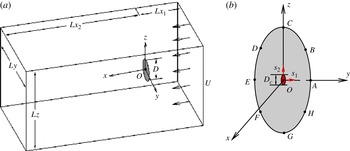
As shown in figure 1(a), we consider a uniform flow over a thin circular flexible plate with a diameter
 $D$
, thickness
 $h$
, density
 ${\it\rho}_{s}$
and Young’s modulus
 $E$
. The plate centre is clamped with a core diameter
 $D_{c}$
. The surrounding fluid has a density
 ${\it\rho}$
and dynamic viscosity
 ${\it\mu}$
. A uniform flow of velocity
 $U$
is perpendicular to the initial plate plane. Here, a local moving curvilinear coordinate system
 $(s_{1},s_{2})$
defined on the plate surface, as shown in figure 1(b), is used to describe the configuration and motion of the plate.
(a) Schematic diagram of the flow over a circular flexible plate and (b) two coordinate systems: a moving curvilinear coordinate system
 $(s_{1},s_{2})$
for the plate and a fixed Cartesian coordinate system
 $(x,y,z)$
for the fluid flow.

The incompressible Navier–Stokes equations are used to describe the fluid flow,
 $$\begin{eqnarray}\displaystyle & \displaystyle \frac{\partial \mathbf{v}}{\partial t}+\mathbf{v}\boldsymbol{\cdot }\boldsymbol{{\rm\nabla}}\mathbf{v}=-\frac{1}{{\it\rho}}\boldsymbol{{\rm\nabla}}p+\frac{{\it\mu}}{{\it\rho}}{\rm\nabla}^{2}\mathbf{v}+\boldsymbol{f}, & \displaystyle\end{eqnarray}$$
 $$\begin{eqnarray}\displaystyle & \boldsymbol{{\rm\nabla}}\boldsymbol{\cdot }\mathbf{v}=0, & \displaystyle\end{eqnarray}$$
 $\mathbf{v}$
is the velocity,
 $p$
the pressure and
 $\boldsymbol{f}$
the body force term. The structural equation with large displacement is used to govern the motion of the plate (Huang & Sung Reference Huang and Sung2010)
 $$\begin{eqnarray}\displaystyle {\it\rho}_{s}h\frac{\partial ^{2}\boldsymbol{X}}{\partial t^{2}}=\mathop{\sum }\limits_{i,j=1}^{2}\left[\frac{\partial }{\partial s_{i}}\!\left(Eh{\it\varphi}_{ij}\!\left[{\it\delta}_{ij}-\!\left(\frac{\partial \boldsymbol{X}}{\partial s_{i}}\cdot \frac{\partial \boldsymbol{X}}{\partial s_{j}}\right)^{-1/2}\right]\!\frac{\partial \boldsymbol{X}}{\partial s_{j}}-\frac{\partial }{\partial s_{j}}\left(EI{\it\gamma}_{ij}\frac{\partial ^{2}\boldsymbol{X}}{\partial s_{i}\partial s_{j}}\right)\right)\!\right]+\boldsymbol{F}_{s}, & & \displaystyle \nonumber\\ \displaystyle & & \displaystyle\end{eqnarray}$$
where
 $\boldsymbol{X}$
is the position vector of the plate,
 $\boldsymbol{F}_{s}$
is the Lagrangian force exerted on the plate by the fluid,
 $Eh$
and
 $EI$
are the stretching and bending stiffness,
 ${\it\varphi}_{ij}$
and
 ${\it\gamma}_{ij}$
are the in-plane and out-of-plane effect matrices, respectively, and
 ${\it\delta}_{ij}$
is the Kronecker delta function. Note that the density
 ${\it\rho}_{s}h$
in (2.3) actually represents the plate area density difference and the actual area density should be
 ${\it\rho}_{s}h+{\it\rho}h$
(Huang & Sung Reference Huang and Sung2010).
The characteristic quantities
 ${\it\rho}$
,
 $U$
and
 $D$
are chosen to non-dimensionalize the above equations. The dimensionless governing parameters are described as follows: the Reynolds number
 $\mathit{Re}={\it\rho}UD/{\it\mu}$
, the stretching stiffness
 $S=Eh/{\it\rho}U^{2}D$
, the bending stiffness
 $K=EI/{\it\rho}U^{2}D^{3}$
, the mass ratio of the plate and the fluid
 $M={\it\rho}_{s}h/{\it\rho}D$
and the clamped core size
 $d=D_{c}/D$
.
To solve (2.1)–(2.3), the initial and boundary conditions are given as follows. A uniform flow (
 $U,0,0$
) is used as an initial condition. A no-slip velocity boundary condition
 $\mathbf{v}=\boldsymbol{V}_{s}$
is applied on the surface of the plate. A uniform velocity
 $U$
is set at the upstream boundary and the side boundaries of the fluid computational domain. A convective boundary condition
 $\partial \mathbf{v}/\partial t+U\partial \mathbf{v}/\partial x=\mathbf{0}$
is specified at the downstream boundary.
3. Numerical method and validation
3.1. Numerical method
The governing equations of the fluid–plate problem are solved numerically by an penalty immersed boundary (IB)–lattice Boltzmann (LB) method for the fluid flow and a finite-element method for the motion of the flexible plate. The IB method has been extensively applied to flow–structure interaction problems (Peskin Reference Peskin1977, Reference Peskin2002; Mittal & Iaccarino Reference Mittal and Iaccarino2005). The body force term
 $\boldsymbol{f}$
in (2.1) is used as an interaction force between the fluid and the boundary to enforce the no-slip velocity boundary condition on the body surface. The Lagrangian interaction force between the fluid and the boundary can be calculated by the penalty strategy (Goldstein, Handler & Sirovich Reference Goldstein, Handler and Sirovich1993; Huang, Shin & Sung Reference Huang, Shin and Sung2007; Huang, Chang & Sung Reference Huang, Chang and Sung2011)
 $$\begin{eqnarray}\displaystyle \boldsymbol{F}_{s}(s_{1},s_{2},t) & = & \displaystyle {\it\alpha}\int _{0}^{t}[\boldsymbol{V}_{f}(s_{1},s_{2},t^{\prime })-\boldsymbol{V}_{s}(s_{1},s_{2},t^{\prime })]\text{d}t^{\prime }\nonumber\\ \displaystyle & & \displaystyle +\,{\it\beta}[\boldsymbol{V}_{f}(s_{1},s_{2},t)-\boldsymbol{V}_{s}(s_{1},s_{2},t)],\end{eqnarray}$$
where
 ${\it\alpha}$
and
 ${\it\beta}$
are parameters which are selected based on the previous studies (Gao & Lu Reference Gao and Lu2008; Tian et al.
Reference Tian, Luo, Zhu, Liao and Lu2011a
; Hua et al.
Reference Hua, Zhu and Lu2013),
 $\boldsymbol{V}_{s}=\partial \boldsymbol{X}/\partial t$
is the plate velocity and
 $\boldsymbol{V}_{f}$
is the fluid velocity at the position of the plate obtained by interpolation
 $$\begin{eqnarray}\boldsymbol{V}_{f}(s_{1},s_{2},t)=\int \mathbf{v}(\boldsymbol{x},t){\it\delta}(\boldsymbol{x}-\boldsymbol{X}(s_{1},s_{2},t))\text{d}\boldsymbol{x}.\end{eqnarray}$$
Then, the Eulerian body force can be calculated as
 $$\begin{eqnarray}\boldsymbol{f}(\boldsymbol{x},t)=-\!\!\iint \boldsymbol{F}_{s}(s_{1},s_{2},t){\it\delta}(\boldsymbol{x}-\boldsymbol{X}(s_{1},s_{2},t))\text{d}s_{1}\text{d}s_{2}.\end{eqnarray}$$
The interaction forces
 $\boldsymbol{F}_{s}(s_{1},s_{2},t)$
and
 $\boldsymbol{f}(\boldsymbol{x},t)$
obtained by (3.1) and (3.3) are applied to (2.3) and (2.1), respectively.
The LB equation has been widely used to simulate complex flows as an alternative to conventional numerical methods for the Navier–Stokes equations (Chen & Doolen Reference Chen and Doolen1998; Tian et al. Reference Tian, Luo, Zhu, Liao and Lu2011a ; Li & Lu Reference Li and Lu2012; Hua et al. Reference Hua, Zhu and Lu2013). The LB equation with the BGK model is
 $$\begin{eqnarray}g_{i}(\boldsymbol{x}+\boldsymbol{e}_{i}{\rm\Delta}t,t+{\rm\Delta}t)-g_{i}(\boldsymbol{x},t)=-\frac{1}{{\it\tau}}[g_{i}(\boldsymbol{x},t)-g_{i}^{eq}(\boldsymbol{x},t)]+{\rm\Delta}tF_{i},\end{eqnarray}$$
where
 ${\it\tau}$
is the non-dimensional relaxation time associated with fluid viscosity,
 ${\rm\Delta}t$
is the time increment and
 $g_{i}(\boldsymbol{x},t)$
is the distribution function for particles with velocity
 $\boldsymbol{e}_{i}$
at position
 $\boldsymbol{x}$
and time
 $t$
. The equilibrium distribution function
 $g_{i}^{eq}$
and the forcing term
 $F_{i}$
(Guo, Zheng & Shi Reference Guo, Zheng and Shi2002) are defined as
 $$\begin{eqnarray}\displaystyle & \displaystyle g_{i}^{eq}={\it\omega}_{i}{\it\rho}\left[1+\frac{\boldsymbol{e}_{i}\boldsymbol{\cdot }\mathbf{v}}{c_{s}^{2}}+\frac{\mathbf{v}\mathbf{v}:(\boldsymbol{e}_{i}\boldsymbol{e}_{i}-c_{s}^{2}\boldsymbol{I})}{2c_{s}^{4}}\right], & \displaystyle\end{eqnarray}$$
 $$\begin{eqnarray}\displaystyle & \displaystyle F_{i}=\left(1-\frac{1}{2{\it\tau}}\right){\it\omega}_{i}\left[\frac{\boldsymbol{e}_{i}-\mathbf{v}}{c_{s}^{2}}+\frac{\boldsymbol{e}_{i}\boldsymbol{\cdot }\mathbf{v}}{c_{s}^{4}}\boldsymbol{e}_{i}\right]\boldsymbol{\cdot }\boldsymbol{f}, & \displaystyle\end{eqnarray}$$
 ${\it\omega}_{i}$
is the weighting factor and
 $c_{s}$
is the speed of sound. The variables velocity
 $\mathbf{v}$
and mass density
 ${\it\rho}$
can be obtained by the distribution functions
 $$\begin{eqnarray}\displaystyle & \displaystyle {\it\rho}=\mathop{\sum }\limits_{i}g_{i}, & \displaystyle\end{eqnarray}$$
 $$\begin{eqnarray}\displaystyle & \displaystyle {\it\rho}\mathbf{v}=\mathop{\sum }\limits_{i}\boldsymbol{e}_{i}g_{i}+\frac{1}{2}\boldsymbol{f}{\rm\Delta}t. & \displaystyle\end{eqnarray}$$
Further, a nonlinear finite-element structural solver designed by Doyle (Reference Doyle1991, Reference Doyle2001) is used to solve (2.3) and a detailed description of the finite-element method is also given by Doyle (Reference Doyle2001). We briefly describe the numerical method following a recent work on dynamic pitching of an elastic rectangular wing (Dai et al. Reference Dai, Luo and Doyle2012). The three-node triangular element describes the plate deformations. Each node of the element has six degrees of freedom, including three displacement components and three angles of rotation. The plate element used is the discrete Kirchhoff triangular element which has been regarded as one of the most efficient flexural elements (Batoz, Bathe & Ho Reference Batoz, Bathe and Ho1980). The large-displacement and small-strain deformation in the structural solver is handled using the corotational scheme. A local coordinate system is envisioned as moving with each discrete element, and the element behaves linearly as described by the Kirchhoff–Love theory of plates in this local coordinate system. Consequently, the geometrical nonlinearities of the original problem are shifted to the coordinate transformation. The time stepping of the nonlinear system of algebraic equations is achieved using an iterative strategy to ensure a second-order accuracy.
Based on our careful convergence studies with different computational domains and lattice spacing, the computational domain for fluid flow is chosen as
 $[-10,30]\times [-10,10]\times [-10,10]$
in the
 $x$
,
 $y$
and
 $z$
directions. A non-uniform mesh technique (He, Luo & Dembo Reference He, Luo and Dembo1996) is employed to solve our problem for improving computational efficiency. The mesh is uniform with a fine spacing 0.025 in the near region of the plate, i.e.
 $[-2,4]\times [-2,2]\times [-2,2]$
, and gradually increases to a coarse spacing 0.1 in the far boundary region. The mesh size increases in a geometric progression. Note that the uniform mesh around the plate is compatible with the IB method (Mittal et al.
Reference Mittal, Dong, Bozkurttas, Najjar, Vargas and Vonloebbecke2008; Dai et al.
Reference Dai, Luo and Doyle2012) and the interpolation kernel function is used as the standard IB method (Peskin Reference Peskin2002). The plate is discretized by approximate 3000 triangular elements. The time step is
 ${\rm\Delta}t=0.0025$
for the simulations of fluid flow and plate deformation.
3.2. Validation
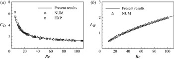
To validate the numerical method and its implementation, we consider viscous flow over a rigid circular plate (Shenoy & Kleinstreuer Reference Shenoy and Kleinstreuer2008). Figure 2 shows the drag coefficient
 $C_{D}$
and the length of the wake
 $L_{W}$
versus the Reynolds number
 $\mathit{Re}$
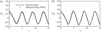
. It is seen that our calculated results agree well with the previous experimental and computational data. Further, we consider a viscous flow over a flexible structure, i.e. a flapping flag in a uniform flow (Huang & Sung Reference Huang and Sung2010). The dimensionless governing parameters are chosen as
 $\mathit{Re}=100$
,
 $M=1$
,
 $K=0.0001$
and
 $S=1000$
with an aspect ratio
 $AR=1$
. Figure 3 shows the time history of the transverse (i.e.
 $y$
direction) displacement of two points on the trailing edge of the flag. It is seen that the present results agree well with the previous ones (Huang & Sung Reference Huang and Sung2010).
Comparison of the present results and previous data for flow over a rigid circular plate: (a) drag coefficient
 $C_{D}$
and (b) length of the wake
 $L_{W}$
, where NUM and EXP represent the numerical (Shenoy & Kleinstreuer Reference Shenoy and Kleinstreuer2008) and experimental (Ross & Willmarth Reference Ross and Willmarth1971) data.

Comparison of the present results and previous data (Huang & Sung Reference Huang and Sung2010) for a flapping flag in a uniform flow: (a) time-dependent transverse (
 $y$
direction) displacement at point A (low corner on the trailing edge) and (b) at point B (mid-point on the trailing edge).

Moreover, the numerical strategy used here has been validated in our previous work and applied with success to a wide range of flows, such as viscous flow past three filaments in side-by-side arrangement (Tian et al. Reference Tian, Luo, Zhu and Lu2011b ), dynamics of flow over flapping plates (Li & Lu Reference Li and Lu2012) and locomotion of flapping flexible plate (Hua et al. Reference Hua, Zhu and Lu2013).
4. Results and discussion
In this section, we present some typical results on the dynamics of fluid flow over a circular flexible plate. The governing parameters used in this study are as follows: the bending stiffness
 $K=10^{-5}{-}0.1$
, the stretching stiffness
 $S=10{-}1000$
, the Reynolds number
 $\mathit{Re}=100$
and 200, the clamped core size
 $d=0.1{-}0.5$
and the mass ratio of the plate and the fluid
 $M=0.1$
and 2. Unless otherwise stated, the mass ratio and the core size are
 $M=0.1$
and
 $d=0.1$
in the following results.
We here analyse the choice of the parameters. The bending stiffness and stretching stiffness are two important parameters to govern the plate deformation. The bending stiffness
 $K=10^{-5}{-}0.1$
is consistent with the experimental range (Schouveiler & Eloy Reference Schouveiler and Eloy2013). During this range, the deformation modes may occur for
 $K<0.1$
and the behaviour of the plate tends to the rigid case for
 $K>0.1$
. The stretching stiffness
 $S=10{-}1000$
allows us to investigate extensible and inextensible effect on the plate deformation with the plate being obviously extensible for
 $S=10$
and nearly inextensible for
 $S=1000$
. The Reynolds number is another important parameter to govern the fluid flow. We considered two Reynolds numbers
 $\mathit{Re}=100$
and 200 which lie in a moderate range with a significant viscous effect. The two cases
 $\mathit{Re}=100$
and 200 correspond to steady and unsteady flow states for flow over a rigid circular plate (Shenoy & Kleinstreuer Reference Shenoy and Kleinstreuer2008). The clamped core size
 $d=0.1$
is chosen based on the experiment (Schouveiler & Eloy Reference Schouveiler and Eloy2013). To examine the effect of the core size on plate deformation, a larger core size is also considered. In addition, the mass ratio
 $M=0.1$
matches with
 $M\sim O(10^{-2})$
for the case of a polysiloxane plate in water tunnel (Schouveiler & Eloy Reference Schouveiler and Eloy2013) and
 $M=2$
with
 $M\sim O(1)$
for the case of a plate in the wind tunnel (Kim et al.
Reference Kim, Cossé, Huertas Cerdeira and Gharib2013).
4.1. Deformation modes
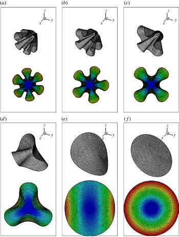
Based on a series of simulations for a wide range of parameters considered here, we have identified six distinct modes of the plate deformation due to the fluid–structure interaction in terms of the number of azimuthal folds, i.e. axial symmetry (or zerofold), twofold, threefold, fourfold, fivefold and sixfold patterns, which can be briefly called 0F, 2F, 3F, 4F, 5F and 6F modes, respectively. Figure 4 shows the six modes for different values of
 $K$
. It is seen that the fold number increases from 0F (axial symmetry) to 6F as
 $K$
decreases. Moreover, the peripheral size of each fold in a multifold mode looks almost the same, indicating that the folds appear to be periodically arranged along the azimuthal direction.
Deformation of the plate for six typical modes with
 $\mathit{Re}=100$
,
 $S=100$
and (a)
 $K=10^{-5}$
, (b)
 $K=4\times 10^{-5}$
, (c)
 $K=10^{-4}$
, (d)
 $K=5\times 10^{-4}$
, (e)
 $K=0.01$
and ( f)
 $K=0.05$
, corresponding to 6F, 5F, 4F, 3F, 2F and 0F, respectively. The upper pattern is the three-dimensional view and the lower one is the pattern coloured by the streamwise (
 $x$
direction) displacement contours on the
 $y{-}z$
plane.

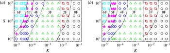
An overview of the six deformation modes on the
 $K{-}S$
plane is shown in figure 5 for two typical Reynolds numbers
 $\mathit{Re}=100$
and 200, which correspond to steady and unsteady states for flow over a rigid circular plate (Shenoy & Kleinstreuer Reference Shenoy and Kleinstreuer2008), respectively. It is identified that the critical value
 $K$
separating two neighbouring modes essentially increases as
 $S$
increases. Comparison of figure 5(a,b) shows that the classification of modes looks qualitatively similar. Recently, Schouveiler & Eloy (Reference Schouveiler and Eloy2013) have experimentally investigated the effect of
 $K$
on the draping mode and analytically introduced a Cauchy number
 $C_{Y}$
to distinguish different deformation modes. Four draping modes, denoted by C, 2F, 3F and
 $3\text{F}^{\ast }$
, are experimentally identified for
 $C_{Y}=1800{-}0.003$
, corresponding to
 $K=1.7\times 10^{-5}{-}10$
, where C mode is a cylindrical shape and
 $3\text{F}^{\ast }$
mode is a bent threefold cone. In this paper, the C and 2F modes are collectively called the 2F mode. The critical value
 $K$
separating the 2F and 3F modes is essentially consistent with the experimental data (Schouveiler & Eloy Reference Schouveiler and Eloy2013). Furthermore, our numerical simulations have revealed more deformation modes, i.e. modes with greater number of folds in the configuration of the deformed plate. The relevant reason may be associated with the larger clamped core size used here and the effect of the clamped core size on the fold number will be further analysed in § 4.4. On the other hand, as a low-Reynolds-number flow is considered, the considerable viscous force which is tangential to the plate surface is generated. Similar to the effect of a surface tangential component of gravity (Cerda et al.
Reference Cerda, Mahadevan and Pasini2004), the viscous force can provide a favourable work to form more fold number during the draping.
Overview of the six typical deformation mode regions in the
 $K{-}S$
plane for (a)
 $\mathit{Re}=100$
and (b)
 $\mathit{Re}=200$
.

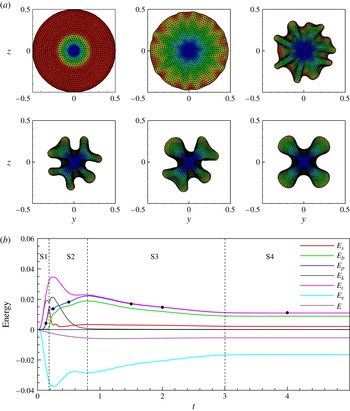
To gain better insight into the plate deformation, the developing process of deformation modes is investigated. As a typical case, figure 6(a) shows the developing process of deformation for the 4F mode. It is identified that the process can be qualitatively divided into four typical stages, including: S1 (i.e. stage 1), the plate changing from a flat shape to an axisymmetric shape with very small deformation; S2, the plate deforming into a draping shape with more folds; S3, the plate adjusting the folds; and S4, the plate evaluating to a final state. Thus, the patterns shown in figure 6(a) correspond to the four stages, i.e. S1 at
 $t=0.125$
, S2 at
 $t=0.25$
and 0.5, S3 at
 $t=1.5$
and 2 and S4 at
 $t=4$
, which are marked in figure 6(b).
Developing process of the plate deformation pattern coloured by the streamwise displacement contours (a) and energy evolution (b) for
 $\mathit{Re}=100$
,
 $S=100$
and
 $K=10^{-4}$
. The instants of the six patterns in (a) are marked in (b) by black points, i.e.
 $t=0.125$
, 0.25, 0.5, 1.5, 2 and 4.

Since the plate is flexible, it can store elastic potential energy in deformation. The stretching energy is defined as
 $E_{s}(t)=S/2\iint \sum _{i,j=1}^{2}{\it\varphi}_{ij}[(\partial \boldsymbol{X}/\partial s_{i}\cdot \partial \boldsymbol{X}/\partial s_{j})^{1/2}-{\it\delta}_{ij}]^{2}\text{d}s_{1}\text{d}s_{2}$
, the bending energy as
 $E_{b}(t)=K/2\iint \sum _{i,j=1}^{2}{\it\gamma}_{ij}\partial ^{2}\boldsymbol{X}/\partial s_{i}^{2}\cdot \partial ^{2}\boldsymbol{X}/\partial s_{j}^{2}\text{d}s_{1}\text{d}s_{2}$
. The total elastic potential energy is then
 $E_{p}(t)=E_{s}(t)+E_{b}(t)$
. Moreover, the kinetic energy of the plate is defined as
 $E_{k}(t)=M/2\iint V_{s}^{2}(s_{1},s_{2},t)\text{d}s_{1}\text{d}s_{2}$
. Figure 6(b) shows the evolution of these energies. The developing process of plate deformation is accompanied by the energy exchanges. The potential energy
 $E_{p}$
has the most contribution from
 $E_{s}$
and increases rapidly in S1. Then
 $E_{s}$
decreases and
 $E_{b}$
increases in S2. Further,
 $E_{s}$
is almost unchanged and
 $E_{b}$
decreases gradually. Finally, both
 $E_{s}$
and
 $E_{b}$
remain nearly constant in S4. Furthermore, the kinetic energy
 $E_{k}$
increases quickly in S1 and decreases quickly in S2, and becomes negligibly small in S3 and S4.
The system energy is further analysed by considering the energy in the fluid domain. The kinetic energy with respect to the free-stream fluid flow is defined as
 $E_{v}={\textstyle \frac{1}{2}}\int _{CV}{\it\rho}(\mathbf{v}\boldsymbol{\cdot }\mathbf{v}-U^{2})\text{d}V$
, where
 $CV$
represents the control volume including the vortex wake which is chosen as the computational domain here. Then, the system energy is defined as
 $E=E_{t}+E_{v}$
. It is seen from figure 6(b) that the system energy
 $E$
decreases gradually and then remains nearly constant during the plate deformation process in S3 and S4 as demonstrated in figure 6(a). The system energy loss is physically related to the viscous dissipation of fluid flow.
4.2. System states and vortical structures
From the preceding description of the developing process of deformation mode, it is desirable to study the state of the fluid–structure system at the final stage, i.e. steady or unsteady state, which is also related to the vortex shedding from the plate. Thus, we here investigate the system state and the vortical structures in the wake of the plate.
Our simulations of flow over a thin circular rigid disk show that the flow state is steady for
 $\mathit{Re}=100$
and unsteady for
 $\mathit{Re}=200$
, consistent with previous results (Shenoy & Kleinstreuer Reference Shenoy and Kleinstreuer2008). Further, considering flow over a flexible plate, we have identified that the flow state is always steady at
 $\mathit{Re}=100$
for all cases shown in figure 5(a), and can be steady or unsteady at
 $\mathit{Re}=200$
depending on the bending rigidity. Based on our simulations shown in figure 5(b), it is found that the flow state is unsteady for the 0F and 2F modes, and steady for the 3F, 4F, 5F and 6F modes at
 $\mathit{Re}=200$
. Such mode classification regions for the steady and unsteady states may be understood in terms of the effective Reynolds number. As shown in figure 4, the deformation of the plate for 3F, 4F, 5F and 6F modes is larger compared with the deformation for 0F and 2F modes. Then, the deformed plate becomes more streamlined and its projected area is reduced, resulting in the decrease of the effective Reynolds number. Therefore, we can reasonably conclude that the unsteadiness at
 $\mathit{Re}=200$
does not modify more drastically the mode regions compared with
 $\mathit{Re}=100$
, i.e. unsteady state for the 0F and 2F modes and steady state for the other modes.
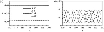
To demonstrate the final state of the deformed plate, figure 7 shows the streamwise (i.e.
 $x$
direction) displacements of eight points on the edge of plate marked in figure 1(b) for two typical cases. As shown in figure 7(a) for
 $K=10^{-4}$
, corresponding to the 4F mode in figure 5(b), it is obvious that the state of plate deformation is steady. From figure 7(b) for
 $K=10^{-2}$
with the 2F mode, it is reasonably identified that the plate vibrates periodically, indicating that the state of plate deformation is unsteady.
Streamwise displacement of eight points on the outer edge marked in figure 1(b) for two typical cases with
 $\mathit{Re}=200$
,
 $S=100$
and (a)
 $K=10^{-4}$
and (b)
 $K=10^{-2}$
.

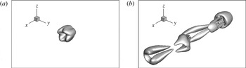
The state of plate deformation is associated with the vortex shedding from the plate due to the fluid–structure interaction. The vortical structures, which are depicted by the isosurface of the
 $Q$
criterion (Jeong & Hussain Reference Jeong and Hussain1995), are shown in figure 8 for the two cases shown in figure 7. It is seen that the vortical structure in figure 8(a) demonstrates a steady petal-like pattern with the same number of deformed folds of the plate. For the unsteady state, there exists regular shedding of double-sided hairpin-shaped vortex structure in figure 8(b), which is similar to the pattern for flow over a rigid circular plate. Further, we have identified that the vortex shedding frequency is consistent with the plate vibration frequency. The Strouhal number defined as
 $\mathit{St}=fD/U$
is calculated as 0.105 for the case in figure 7(b), which is close to the counterpart value 0.113 for flow over a rigid plate (Shenoy & Kleinstreuer Reference Shenoy and Kleinstreuer2008). Furthermore, for a circular plate with clamped centre and free outer edge, the natural frequency can be estimated by
 $f_{N}=2K_{n}/({\rm\pi}D^{2})\sqrt{EI/({\it\rho}_{s}h)}$
(Leissa Reference Leissa1969) and obtained as
 $O(10^{-1})$
based on the parameters in figure 7(b). Thus, the plate vibration frequency is deviated from its natural frequency and is the same as the vortex shedding frequency. This behaviour is reasonably associated with the forced system response.
Vortical structures visualized by an isosurface of the
 $Q$
criterion with
 $Q=0.01$
for
 $\mathit{Re}=200$
,
 $S=100$
and (a)
 $K=10^{-4}$
and (b)
 $K=10^{-2}$
.

4.3. Drag reduction and elastic potential energy
For fluid flow over a flexible plate, the drag reduction related to the plate deformation and the elastic potential energy of the flexible plate are two important concerns for many relevant problems (e.g. Schouveiler & Boudaoud Reference Schouveiler and Boudaoud2006; Gosselin et al. Reference Gosselin, de Langre and Machado-Almeida2010; Hua et al. Reference Hua, Zhu and Lu2013). We address these two issues here for our specific problem.
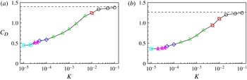
Figure 9 shows the drag coefficient
 $C_{D}$
versus
 $K$
with
 $S=100$
for
 $\mathit{Re}=100$
and 200. Note that
 $C_{D}$
represents the mean value of drag for unsteady cases. It is noted that the
 $C_{D}$
of the flexible plate is always less than that of the rigid plate and the
 $C_{D}$
decreases as
 $K$
decreases (i.e. more flexible). As shown in figure 5, the plate deformation patterns are dependent on different values of
 $K$
. Thus, the mechanism of drag reduction is reasonably related to the projected area reduction and shape streamlining of the deformed plate (Vogel Reference Vogel1996). Further, the curve of drag coefficient with respect to
 $K$
is piecewise smooth. The non-smoothness occurs at the switch of deformation modes.
Drag coefficient versus the bending stiffness
 $K$
for
 $S=100$
and (a)
 $\mathit{Re}=100$
and (b)
 $\mathit{Re}=200$
. The dashed line represents the
 $C_{D}$
of rigid plate for the same Reynolds number. The symbols represent the different deformation modes shown in figure 5.

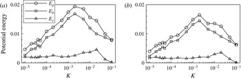
Figure 10 shows the profiles of the mean potential energies defined in § 4.1. It is obtained that
 $E_{b}$
is greater than
 $E_{s}$
and has the greatest contribution to the total potential energy
 $E_{p}$
. The energy
 $E_{s}$
does not change much for
 $K<10^{-2}$
, then reaches a maximum at
 $K=0.02$
, and finally decreases with
 $K$
. The energy
 $E_{b}$
increases with
 $K$
until it reaches a peak at
 $K=2\times 10^{-3}$
, and then decreases as
 $K$
increases further.
Potential energy versus the bending stiffness
 $K$
for
 $S=100$
and (a)
 $\mathit{Re}=100$
and (b)
 $\mathit{Re}=200$
.

Furthermore, compared with the profiles in figure 10(a,b), it is identified that the potential energies for
 $\mathit{Re}=100$
are essentially larger than the counterparts for
 $\mathit{Re}=200$
. This behaviour may be related to the fact that larger drag or larger flow load at lower Reynolds number, as shown in figure 9, results in greater deformation. Therefore, more potential energy is generated and stored in the deformed plate.
4.4. Effects of clamped core size and mass ratio
All of the above results are obtained from simulations using different bending stiffness
 $K$
, stretching stiffness
 $S$
and Reynolds number
 $\mathit{Re}$
but fixed core size (
 $d=0.1$
) and mass ratio (
 $M=0.1$
). To examine the effects of
 $d$
and
 $M$
on the deformation modes, we further perform some simulations using different values of
 $d$
and
 $M$
.
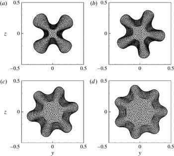
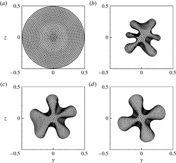
Figure 11 shows the plate deformation patterns for several clamped core sizes. It is interesting to note that the fold number increases with the core size. Relevant studies on deformation of the thin elastic sheets have been performed experimentally (Cerda, Ravi-Chandar & Mahadevan Reference Cerda, Ravi-Chandar and Mahadevan2002) and theoretically (Cerda & Mahadevan Reference Cerda and Mahadevan2003). They proposed a formula to estimate the deformed winkling wavelength of an elastic sheet under a uniaxial tensile strain, i.e.
 ${\it\lambda}=2\sqrt{{\rm\pi}}(EI/T)^{1/4}L^{1/2}$
, where
 $T$
is the tension along the sheet and
 $L$
is length scale of the sheet. Further, Cerda et al. (Reference Cerda, Mahadevan and Pasini2004) analysed the gravity-induced draping of a circular tablecloth with a diameter
 $D$
on a circular table and estimated the fold number as
 $n\sim D/{\it\lambda}$
. In a typical case, they theoretically predicted
 $n\approx 15$
for the tablecloth draping, which is qualitatively aligned with
 $n=10$
in their observations. In the present study, the bending stiffness is
 $EI=K{\it\rho}U^{2}D^{3}$
, the length scale is
 $L=D-D_{c}$
, and the tension is given by
 $T\sim 1/\sqrt{\mathit{Re}}S{\it\rho}U^{2}D^{2}/L$
. Then, the fold number can be expressed as
 $n\sim D/{\it\lambda}\sim 1/(2\sqrt{{\rm\pi}})S^{1/4}\mathit{Re}^{-1/8}K^{-1/4}(1-d)^{-3/4}$
. This expression reasonably predicts the characteristics versus the relevant parameters; it suggests that the fold number
 $n$
increases as the increase of
 $d$
and
 $S$
and also increases as the decrease of
 $K$
and
 $\mathit{Re}$
, consistent with the results shown in figures 5 and 11.
Effect of the core size on the deformation pattern for
 $\mathit{Re}=100$
,
 $M=0.1$
,
 $S=100$
,
 $K=10^{-4}$
and (a)
 $d=0.1$
, (b)
 $d=0.2$
, (c)
 $d=0.3$
and (d)
 $d=0.5$
.

Further, to examine the performance of the theoretical analysis and the effect of the core size
 $d$
on the fold number
 $n$
, we can directly express
 $n=C(1-d)^{-3/4}$
with
 $C=1/(2\sqrt{{\rm\pi}})S^{1/4}\mathit{Re}^{-1/8}K^{-1/4}$
and obtain
 $C=5.02$
in terms of the parameters
 $\mathit{Re}=100$
,
 $S=100$
and
 $K=10^{-4}$
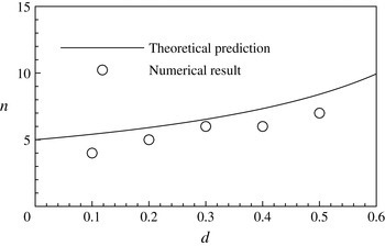
used in figure 11. Then, figure 12 shows the comparison of fold number obtained by the present numerical simulation and theoretical prediction. The reliable agreement also supports the theoretical analysis (Cerda & Mahadevan Reference Cerda and Mahadevan2003; Cerda et al.
Reference Cerda, Mahadevan and Pasini2004) and is helpful in understanding the physical mechanisms on the plate deformation modes.
Comparison of the fold number obtained by the numerical simulation and theoretical prediction.

To investigate the effect of the mass ratio on the deformation mode, we have performed some simulations with different mass ratios and found that greater mass ratio does not alter the final deformation pattern but only delays the developing process of deformation into its final state. For example, figure 13 shows the developing process of the plate deformation for
 $M=2$
with the same other parameters as in figure 6(a). It is identified that the plate deformation reaches its final state at approximately
 $t=30$
for
 $M=2$
, while it does so at
 $t=4$
for
 $M=0.1$
.
Developing process of the deformation patterns for
 $M=2$
with other parameters being the same as those used in figure 6. The instants of the four patterns correspond to
 $t=0.5$
, 3, 15 and 30, respectively.

We have also examined the unsteady modes (i.e. 0F and 2F) at
 $\mathit{Re}=200$
for
 $M=2$
. As a typical case, we analyse the evolution of deformation mode for
 $M=2$
with the same other parameters as in figure 7(b). It is reasonably obtained that the state of plate deformation is unsteady, which is consistent with the time-dependent deformation for
 $M=0.1$
in figure 7(b). The plate vibration frequency or the vortex shedding frequency is approximately 0.1 for
 $M=2$
which also matches with 0.105 for
 $M=0.1$
.
Further, we have investigated the effect of the mass ratio on the steady and unsteady modes at
 $\mathit{Re}=200$
. Based on the classification of deformation modes in the
 $K{-}S$
plane in figure 5(b), we have also simulated a series of cases for
 $M=2$
at
 $S=100$
. It is identified that the value separating the steady and unsteady regions for
 $M=2$
is consistent with that for
 $M=0.1$
, i.e. the unsteady state for 0F and 2F modes and the steady state for other modes. This behaviour is also consistent with the experimental finding that the mass ratio has negligible effect on the flapping dynamics of an inverted flag, i.e. a free leading edge and a fixed trailing edge of a flexible plate (Kim et al.
Reference Kim, Cossé, Huertas Cerdeira and Gharib2013).
5. Concluding remarks
The dynamics of fluid flow over a circular flexible plate have been studied numerically. Various fundamental mechanisms dictating the relevant behaviours, including plate deformation modes, steady and unsteady states of the system, vortical structures, drag reduction and elastic potential energy of the deformed plate, were examined systematically and are summarized briefly as follows.
Based on a series of simulations for a wide range of parameters considered here, we have found a variety of distinct modes of plate deformation with the azimuthal fold number from axial symmetry to multifold patterns. The diagram of the deformation modes is obtained on the
 $K$
–
 $S$
plane. The critical value
 $K$
separating two neighbouring modes essentially increases as
 $S$
increases. The developing process of plate deformation modes is analysed and found to be qualitatively divided into four typical stages. Moreover, there exist steady and unsteady states of the fluid–structure system. The vortical structures are demonstrated which are closely related to the motion and deformation of the plate.
Further, the drag reduction related to the plate deformation and the elastic potential energy of the flexible plate are investigated. The mechanism of drag reduction is associated with the projected area reduction and shape streamlining of the deformed plate. The elastic potential energy of the flexible plate is analysed. The bending energy is greater than the stretching energy and contributes most to the total elastic potential energy. Moreover, the effects of the clamped core size and mass ratio on the deformation modes are studied. The mass ratio only changes the developing process of the plate deformation and has no effect on its final state. It is found that the fold number increases with the core size. Finally, theoretical analysis is performed and is helpful in understanding the physical mechanisms on the dynamics of the fluid–structure system.
Acknowledgements
This work was supported by the Natural Science Foundation of China (grant no. 11372304) and the 111 Project (grant no. B07033).