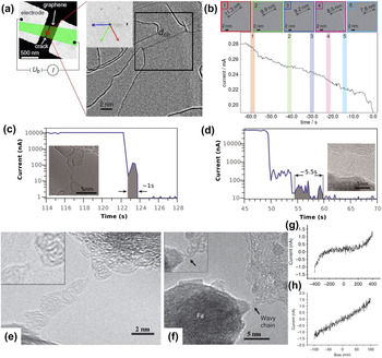
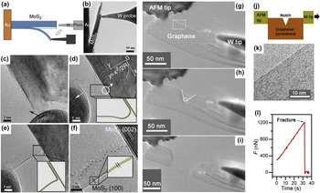
I. INTRODUCTION
Graphene, as the first 2D atomic crystal, Reference Novoselov, Geim, Morozov, Jiang, Zhang, Dubonos, Grigorieva and Firsov1 possesses supreme properties, such as extreme mechanical strength, excellent electronic and thermal conductivities, high surface area, and impermeability to gas. Reference Geim2 Given these properties, graphene is feasible for applications in various fields, including electronics, photonics, composite materials, paints and coatings, energy generation and storage, sensors and metrology, and bioapplications. Reference Novoselov, Fal'ko, Colombo, Gellert, Schwab and Kim3 However, graphene is unlikely to be used for fabricating high-performance integrated logic circuits because of the absence of a band gap. Scientists have explored alternative materials, including structurally related 2D materials, such as hexagonal boron nitride (h-BN), Reference Han, Wu, Zhu, Watanabe and Taniguchi4 transition metal dichalcogenides, Reference Zeng, Yin, Huang, Li, He, Lu, Boey and Zhang5 layered transition oxides, and topological insulators of bismuth telluride (Bi2Te3) and bismuth selenide (Bi2Se3), which have gained extensive interest. Reference Xu, Liang, Shi and Chen6 Like graphene, these 2D materials are important in various applications because of their distinct properties. Since the novel 2D materials will function significantly in the future development of materials, discovering the essential relationship between their structure and properties is vital.
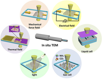
Transmission electron microscope (TEM) has undergone remarkable development, and achieved atomic resolution by the inclusion of aberration correctors and other techniques, such as monochromators, in recent years. Reference Freitag, Kujawa, Mul, Ringnalda and Tiemeijer7–Reference Hutchison, Titchmarsh, Cockayne, Doole, Hetherington, Kirkland and Sawada9 TEM has become an indispensable tool for detailed characterization of the atomic structures of 2D materials. With a full understanding of atomic structures of 2D materials, further investigating the structural evolution and structure–property relationships in a real environment is feasible. We can simulate a real environment by introducing external fields, such as electron irradiation, thermal excitation, electrical fields, and mechanical force, into a TEM. These modifications are called in situ TEM experiments. Electron irradiation can be easily realized or expected in TEM. Detailed in situ experiments have been carried out to study electron irradiation induced structural evolution Reference Girit, Meyer, Erni, Rossell, Kisielowski, Yang, Park, Crommie, Cohen, Louie and Zettl10–Reference Warner, Margine, Mukai, Robertson, Giustino and Kirkland15 and nanofabrication Reference Lin, Cretu, Zhou, Suenaga, Prasai, Bolotin, Cuong, Otani, Okada, Lupini, Idrobo, Caudel, Burger, Ghimire, Yan, Mandrus, Pennycook and Pantelides16,Reference Liu, Xu, Wu, Zhang, Yu, Qiu, Hong, Jin, Li, Wang, Sun and Guo17 of 2D materials. Other in situ TEM characterizations can be realized by specialized holders, including scanning tunneling microscope (STM) holders, electrical bias, heating, cooling, mechanical, and liquid cell holders. Reference Ziegler, Graafsma, Zhang and Frenken18
Moreover, with the development of ultrafast imaging, Reference Barwick, Park, Kwon, Baskin and Zewail19–Reference Robertson, Allen, Wu, He, Olivier, Neethling, Kirkland and Warner24 real-time monitoring of dynamic processes, such as chemical reaction, structure reconstruction, defect generation and migration, and property evolution under various external fields, is feasible. In consequence, TEM served as a nanolab for 2D materials. In this article, we review atomic resolution characterization, in situ growth, nanofabrication, and property characterization of 2D materials, such as graphene, h-BN, and transition metal dichalcogenides (TMDs).
II. ATOMIC RESOLUTION CHARACTERIZATION
With the rapid development of modern TEM technology, TEM has become an indispensable tool for characterizing interior Reference Warner, Ruemmeli, Bachmatiuk and Buechner12,Reference Coleman, Lotya, O'Neill, Bergin, King, Khan, Young, Gaucher, De, Smith, Shvets, Arora, Stanton, Kim, Lee, Kim, Duesberg, Hallam, Boland, Wang, Donegan, Grunlan, Moriarty, Shmeliov, Nicholls, Perkins, Grieveson, Theuwissen, McComb, Nellist and Nicolosi25–Reference Jin, Lin, Suenaga and Iijima30 and edge structure, Reference Girit, Meyer, Erni, Rossell, Kisielowski, Yang, Park, Crommie, Cohen, Louie and Zettl10,Reference Alem, Erni, Kisielowski, Rossell, Gannett and Zettl29,Reference Davami, Shaygan, Kheirabi, Zhao, Kovalenko, Ruemmeli, Opitz, Cuniberti, Lee and Meyyappan31,Reference Komsa, Kotakoski, Kurasch, Lehtinen, Kaiser and Krasheninnikov32 defects, Reference Meyer, Kisielowski, Erni, Rossell, Crommie and Zettl14,Reference Komsa, Kotakoski, Kurasch, Lehtinen, Kaiser and Krasheninnikov32–Reference Qiu, Xu, Wang, Ren, Nan, Ni, Chen, Yuan, Miao, Song, Long, Shi, Sun, Wang and Wang39 grain boundaries Reference Najmaei, Liu, Zhou, Zou, Shi, Lei, Yakobson, Idrobo, Ajayan and Lou26,Reference Grantab, Shenoy and Ruoff40–Reference Tsen, Brown, Levendorf, Ghahari, Huang, Havener, Ruiz-Vargas, Muller, Kim and Park42 and stacking Reference Warner, Ruemmeli, Bachmatiuk and Buechner12,Reference Warner, Mukai and Kirkland43,Reference Cong, Li, Zhang and Yu44 of 2D materials at atomic resolution. However, electron irradiation is inevitable and adversely affect the specimen through heating, electrostatic charging, radiolysis, displacement damage, sputtering, and hydrocarbon contamination. Reference Egerton, Li and Malac45 Considering that structural alterations of materials have occasionally been misinterpreted as a structural property, the use of low-voltage TEM equipped with modern aberration correctors for observing 2D materials is important to minimize radiation damage. Reference Xu, Liang, Shi and Chen6,Reference Banhart46 Understanding the atomic structures of 2D materials is of considerable significance for further investigation under different external stimuli.
A. Graphene
As the most investigated representative of the 2D materials, the irradiation effects of graphene have been studied first. Knock-on atom displacements are known as the main source of radiation damage in graphene. Electron beams with an acceleration voltage of 80 kV do not damage graphene, because the maximum energy transferred to a carbon atom is below the theoretical displacement energy. However, this low voltage does not completely eradicate the sputtering of the under-coordinated carbon atom. Recent work has shown that the formation of vacancy defects depends not only on electron energy but also on beam current density. Reference Meyer, Eder, Kurasch, Skakalova, Kotakoski, Park, Roth, Chuvilin, Eyhusen, Benner, Krasheninnikov and Kaiser47 Normally, we still use the TEM at 80 kV to investigate the production, Reference Meyer, Kisielowski, Erni, Rossell, Crommie and Zettl14,Reference Robertson, Allen, Wu, He, Olivier, Neethling, Kirkland and Warner24,Reference Robertson and Warner48 migration, Reference Kotakoski, Mangler and Meyer49 reconstruction, and annihilation Reference Meyer, Kisielowski, Erni, Rossell, Crommie and Zettl14,Reference Robertson, Allen, Wu, He, Olivier, Neethling, Kirkland and Warner24 of defects. Without the special version, the acceleration voltage of TEM in this review is 80 kV.
Given that the unique electronic, thermal, and mechanical properties of graphene are sensitive to lattice structure, Reference Grantab, Shenoy and Ruoff40,Reference Chen, Li, Cullen, Williams and Fuhrer50 the study of defects in graphene is significantly important. Defects in graphene, such as Stone–Wales (SW) defect, monovacancy (MV), divacancy (DV), tetravacancy, multi-vacancies, adatoms, substitutions, interstitials, and grain boundaries, have been explored under electron irradiation.
1. Stone–Wales defect
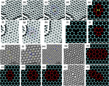
A SW defect is formed by an in-plane 90° rotation of a C–C bond, yielding a transformation of four adjacent hexagons to two pentagons and two heptagons. Reference Robertson and Warner48 The defect is unlikely to remain stable in TEM, because the relaxation energy required for the defect to revert back to pristine lattice is about 5 eV, Reference Li, Reich and Robertson51 which is less than the calculated displacement threshold energy. Reference Li, Reich and Robertson51,Reference Russo and Golovchenko52 As shown in Figs. 1(a)–1(d), an isolated SW defect was found during one exposure of the sequence and relaxed to an unperturbed lattice 4 s later. Reference Meyer, Kisielowski, Erni, Rossell, Crommie and Zettl14
Different defects in graphene. (a–d) SW defect: (a) unperturbed lattice before the appearance of the defect, (b) SW defect, (c) same image with superimposed atomic configuration, and (d) relaxation to unperturbed lattice (after approximately 4 s). (e) Atomic models of SW defect. Yellow bond indicates the reconstructed bond. (f–h) Reconstructed MV: (f) original image and (g) with atomic configuration, and (h) unperturbed lattice, 4 s later. (i–j) Atomic models of the formation of a reconstructed MV: removal of the carbon atom (i) leads to a metastable configuration that can undergo a Jahn–Teller distortion, reconstructing to form the model in (j). Reprinted with permission from Ref. Reference Meyer, Kisielowski, Erni, Rossell, Crommie and Zettl14, Copyright 2008, American Chemical Society. (k–m) TEM images of three different types of DVs: (k) (5–8–5) DV, (l) (555–777) DV, and (m) (5555–6–7777) DV. (n–p) Atomic models corresponding to (k–m), respectively. Reprinted with permission from Ref. Reference Robertson, Allen, Wu, He, Olivier, Neethling, Kirkland and Warner24, Copyright 2012, Macmillan Publishers Limited. (q–r) Two most frequently observed tetravacancy defects and (s–t) their corresponding atomic models. Reprinted with permission from Ref. Reference Robertson, Lee, He, Yoon, Kirkland and Warner53, Copyright 2014, American Chemical Society.

2. Vacancies
The ejection of a carbon atom yields a single vacancy and leaves three dangling bonds in graphene Reference Robertson and Warner48 [Fig. 1(i)]. The MV undergoes a Jahn–Teller distortion Reference Hjort and Stafstrom54 to minimize the energy of the graphene, forming a band between the two atoms near the vacancy and results in a pentagon and a nonagon [Fig. 1(j)]. The images in Figs. 1(f)–1(h) show a single vacancy absorbing a carbon atom and returning to an unperturbed lattice after several seconds. Reference Meyer, Kisielowski, Erni, Rossell, Crommie and Zettl14 A DV is formed by sputtering the carbon atom bonded to only two neighbors in MV, thereby leaving no dangling bonds in the graphene. Reference Robertson and Warner48 This form is more stable under irradiation, because all of the atoms are sp 2 bonded. Several configurations of DV exist and oscillate among each other, Reference Robertson, Allen, Wu, He, Olivier, Neethling, Kirkland and Warner24,Reference Kim, Ihm, Yoon and Lee55 as illustrated in Figs. 1(k)–1(m). With ejection of other two atoms, the tetravacancy was generated under electron irradiation. Robertson et al. Reference Robertson, Lee, He, Yoon, Kirkland and Warner53 examined various structural permutations of tetravacancy defects in monolayer graphene by using aberration-corrected TEM and found that two most prevalent structures are extended line defect structures in Figs. 1(q) and 1(r). Not only the formation energy, but also the specific procedure of tetravacancy formation affects the structures of tetravacancy. Reference Robertson, Lee, He, Yoon, Kirkland and Warner53 The formation of multi-vacancies in graphene can be explained by vacancies migrating and agglomerating with electron beam-induced bond rotation and atom removal. Reference Kotakoski, Krasheninnikov, Kaiser and Meyer34 Continuous sputtering of atoms in a small area will create a hole in graphene with unsaturated bonds around its circumference. The fabrication and healing of holes in graphene and their potential applications will be discussed in the following nanofabrication section.
3. Adatoms, substitutions, and interstitials
There are three main manners for the dopant atoms to incorporate into graphene lattices and tune their properties: adatoms, substitutions, and interstitials.
Adatoms are typically absorbed to the graphene lattice by van der Waals bonding in the bridge (B), hollow (H), and top (T) sites. Reference Robertson and Warner48,Reference Robertson and Warner56 The foreign atom substituting a carbon atom in the graphene lattice, forming bonds with the surrounding carbon atoms, is substitution.
Vacancies can act as occupancy sites for interstitial impurities to form single-atom dopants that are covalently bonded in the lattice. For instance, a DV in graphene is occupied by a surface iron (Fe) contaminant, Reference Robertson, Montanari, He, Kim, Allen, Wu, Olivier, Neethling, Harrison, Kirkland and Warner57 forming an interstitial defect, and trivacancy occupied by a platinum (Pt) interstitial. Reference Wang, Wang, Cheng, Li, Yao, Zhang, Dong, Wang, Schwingenschloegl, Yang and Zhang58
The doped graphene and migration of dopant under electron irradiation will be elaborated later.
4. Grain boundaries
Chemical vapor deposition (CVD) is an excellent and widely used technique for growing large-area graphene. However, this method may introduce grain boundaries, which influence the characteristics of graphene. Thus, investigating grain boundaries, understanding their structure and structure–property relationship, and ultimately engineering grain boundaries to achieve desired properties for future applications are important. Given that various theoretical investigations Reference Grantab, Shenoy and Ruoff40,Reference Liu and Yakobson59–Reference Yazyev and Louie62 on grain boundaries have been conducted, experimentally studying grain boundaries is currently feasible with TEM modern techniques, including scanning TEM (STEM), and high-resolution TEM (HRTEM). The atomic arrangements of grain boundaries can be imaged through STEM and HRTEM.
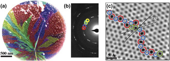
Grain orientations can be mapped by dark field TEM (DF–TEM), in which individual crystal orientations (gained by selected-area electron diffraction patterns) are isolated by using an aperture to select the appropriate diffraction spot, as shown in Figs. 2(a) and 2(b). Reference Huang, Ruiz-Vargas, van der Zande, Whitney, Levendorf, Kevek, Garg, Alden, Hustedt, Zhu, Park, McEuen and Muller41,Reference An, Voelkl, Suk, Li, Magnuson, Fu, Tiemeijer, Bischoff, Freitag, Popova and Ruoff63–Reference Kurasch, Kotakoski, Lehtinen, Skákalová, Smet, Krill, Krasheninnikov and Kaiser66 In Fig. 2(c), STEM (operating at 60 kV) image shows the grain boundary between two graphene grains, which have an angle of 27° at atomic resolution. The grain boundary is composed of different defects, like pentagons, heptagons, and distorted hexagons, which are irregularly arranged. Reference Huang, Ruiz-Vargas, van der Zande, Whitney, Levendorf, Kevek, Garg, Alden, Hustedt, Zhu, Park, McEuen and Muller41 The high concentration of defects at the grain boundaries make the grain boundary more chemically reactive than pristine graphene, Reference Malola, Häkkinen and Koskinen60 and offer sites for adsorbates to bind. Reference Huang, Ruiz-Vargas, van der Zande, Whitney, Levendorf, Kevek, Garg, Alden, Hustedt, Zhu, Park, McEuen and Muller41,Reference An, Voelkl, Suk, Li, Magnuson, Fu, Tiemeijer, Bischoff, Freitag, Popova and Ruoff63
(a) False color dark-field TEM image of multiple graphene grain orientations. (b) Diffraction pattern of polycrystalline graphene in (a), with the colored circles corresponding to the selected aperture used to highlight the same colored grain in (a). (c) Two grains (bottom left, top right) intersect with a 27° relative rotation. Reprinted with permission from Ref. Reference Huang, Ruiz-Vargas, van der Zande, Whitney, Levendorf, Kevek, Garg, Alden, Hustedt, Zhu, Park, McEuen and Muller41, Copyright 2011, Macmillan Publishers Limited.

The grain boundaries mentioned above are arranged by direct atomic bonding, while a distinct configuration existed in a few-layer graphene is overlapping, which one graphene domain grows on the top of a neighboring domain. Reference Robertson, Bachmatiuk, Wu, Schaeffel, Rellinghaus, Buechner, Ruemmeli and Warner65 The two different types of grain boundaries can be distinguished by analyzing the change of diffraction through the grain boundary and the effect of defocus on the contrast of the interface. Overlapping graphene sheets exist an area of superposition of crystal orientations across the grain boundary, Reference Kim, Lee, Regan, Kisielowski, Crommie and Zettl64 and have strong edge contrast with the change of defocus values. Reference Robertson, Bachmatiuk, Wu, Schaeffel, Rellinghaus, Buechner, Ruemmeli and Warner65
5. Edge structure
Three main configurations of edges in graphene exist, namely, zigzag, armchair, and reconstructed (pentagon–heptagon) zigzag and klein edges. Reference Robertson and Warner48,Reference Klein67 Investigating the dynamics of graphene edges is of considerable significance as edge structures, properties, and their functionalization crucially influence the conductive, mechanical, elastic, and chemical properties of graphene nanoribbons.
In theory, graphene sheets with zigzag edges are not stable compared with that of the graphene sheets with armchair edges. Reference Kotakoski, Santos-Cottin and Krasheninnikov68,Reference Koskinen, Malola and Häkkinen69 Experimentally, Kim et al. Reference Kim, Coh, Kisielowski, Crommie, Louie, Cohen and Zettl70 fabricated clean and atomically smooth graphene edges in zigzag, armchair, and reconstructed zigzag configurations by electron beam-induced mechanical tearing. They found that the zigzag edge can be completely and reversibly transform between the hexagon–hexagon zigzag edge and pentagon–heptagon reconstructed zigzag edge under electron irradiation, while the armchair edge is relatively stable, with short zigzag edge segments embedded.
Notably, Girit et al. Reference Girit, Meyer, Erni, Rossell, Kisielowski, Yang, Park, Crommie, Cohen, Louie and Zettl10 and Warner et al. Reference Warner, Ruemmeli, Ge, Gemming, Montanari, Harrison, Buechner and Briggs71 demonstrated that the zigzag edge of the hole is more stable than the armchair edge under electron irradiation at 80 kV. Reference Girit, Meyer, Erni, Rossell, Kisielowski, Yang, Park, Crommie, Cohen, Louie and Zettl10 Koskinen et al. Reference Koskinen, Malola and Häkkinen11 analyzed the data from the successful experiment taken by Girit et al. Reference Girit, Meyer, Erni, Rossell, Kisielowski, Yang, Park, Crommie, Cohen, Louie and Zettl10 and demonstrated the existence and stability of the reconstructed zigzag edge, which is the most stable graphene edge. These results vary considerably from other theoretical and experimental findings of an open edge mentioned above. The reason is that, there are under-coordinated carbon atoms at the rim of the graphene hole with an equal probability to be sputtered, which results in the zigzag edges. Reference Kotakoski, Santos-Cottin and Krasheninnikov68
Graphene edges functionalized by hydrogen are the most elusive to study because of the small atomic mass of hydrogen. In theory, unlike hydrogen attachment, hydrogen-free armchair edges undergoes strong reconstruction and leads to a reduction of the bond lengths, which is likely to form a triple bond. Reference Kawai, Miyamoto, Sugino and Koga72 Therefore, He et al. Reference He, Lee, Robertson, Yoon and Warner73 first indirectly determined whether graphene edges are hydrogenated by measuring the C–C bond lengths in armchair graphene edges and demonstrated that the graphene edges are not always hydrogenated. Furthermore, the group tracked the bond lengths in real time, and found that the lengths increased when the armchair edge being functionalized by an additional atom and form a triangle–hexagon structure while decreased to the same C–C bond upon the removal of the additional atom.
However, there are various defects and chemical functionalization upon the graphene edges, which make the edge structure not perfect. Reference Kim, Coh, Kisielowski, Crommie, Louie, Cohen and Zettl70 Heat treatment can reduce the amount of defects near all edges of graphene, and most of the thermally treated graphene edges are completely closed due to the reduced number of dangling carbon bonds. Reference Liu, Suenaga, Harris and Iijima74 For open edges under high-temperature annealing, most of the configurations are armchair-type, whereas the zigzag-type comprise the least configurations. Reference Westenfelder, Meyer, Biskupek, Kurasch, Scholz, Krill and Kaiser75
Studies about atomic structures of graphene have important significance for understanding and optimizing the properties of graphene, which provide a building block for realizing the ultimate promise of fabricating various devices for future applications.
B. Other 2D materials
Since the discovery of the extraordinary properties of graphene, a diverse source of 2D layered materials, such as h-BN, MoS2, MoSe2, tungsten disulfide (WS2), and other 2D compounds, has boosted great interest. These materials offer unique properties that differ from those of graphene and would be useful in applications ranging from electronics to energy storage.
1. Boron nitride (BN)
h-BN presents the closest structural similarity to graphene, consisting of equal numbers of boron and nitrogen atoms in a honeycomb arrangement. However, the slightly ionic bonding in- and out-of-plane, and its electrically insulating characteristic with a large band gap distinguish h-BN from graphene. Reference Watanabe, Taniguchi and Kanda76 Furthermore, unlike the ABA stacking of graphite, h-BN layers are stacked by AAA structure, which the boron and nitrogen atoms stack directly on top of each other. Reference Alem, Erni, Kisielowski, Rossell, Gannett and Zettl29 Ultrahigh resolution TEM has been applied to identify the structures, defects, and grain boundaries of h-BN. Single-layer h-BN can be fabricated by employing high-energy electron beam to sputter off subsequent layers one-by-one from BN membranes. Reference Jin, Lin, Suenaga and Iijima30,Reference Meyer, Chuvilin, Algara-Siller, Biskupek and Kaiser37
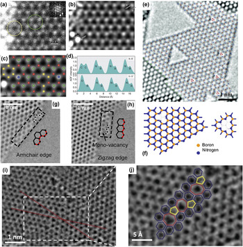
Directly identifying the boron and nitrogen atoms is necessary so that the lattice defects, edge structure, and grain boundaries in h-BN can be clarified. In recent works, individual boron and nitrogen atoms can be discriminated by the intensity profile of TEM reconstructed phase images Reference Alem, Erni, Kisielowski, Rossell, Gannett and Zettl29,Reference Jin, Lin, Suenaga and Iijima30 and STEM annular dark field (STEM–ADF) images Reference Krivanek, Chisholm, Nicolosi, Pennycook, Corbin, Dellby, Murfitt, Own, Szilagyi, Oxley, Pantelides and Pennycook77 [Figs. 3(a)–3(d)]. In these representations, nitrogen yields stronger intensity than boron.
(a) Original and (b) smoothed STEM–ADF images of monolayer BN and (c) with an overlaid structural model: Red, Boron; yellow, Carbon; green, Nitrogen; blue, Oxygen. (d) Line profiles of the image intensity along X–X′ and Y–Y′ in image (b). Reprinted with permission from Ref. Reference Krivanek, Chisholm, Nicolosi, Pennycook, Corbin, Dellby, Murfitt, Own, Szilagyi, Oxley, Pantelides and Pennycook77, Copyright 2010, Macmillan Publishers Limited. (e) Single-layer h-BN membrane with different sizes of triangle-shaped vacancies. Red triangles indicate the boron monovacancies. Reprinted with permission from Ref. Reference Meyer, Chuvilin, Algara-Siller, Biskupek and Kaiser37, Copyright 2009, American Chemical Society. (f) Schematic morphology of the boron MV and the smallest triangle-shaped vacancy. (g–h) HRTEM images of BN edge structures: (g) Zigzag edge and (h) armchair edge. Reprinted with permission from Ref. Reference Alem, Erni, Kisielowski, Rossell, Gannett and Zettl29, Copyright 2009, American Physical Society. (i) Grain boundary in a monolayer of h-BN with a misorientation angle of 21°. (j) Magnified grain boundary defect structure from the inset of (i), hexagon, heptagon, and pentagon structures are depicted in blue, red, and yellow, respectively. Reprinted with permission from Ref. Reference Gibb, Alem, Chen, Erickson, Ciston, Gautam, Linck and Zettl35, Copyright 2013, American Chemical Society.

The threshold energy for the knock-on damage of boron and nitrogen atoms is 74 and 84 keV, Reference Zobelli, Gloter, Ewels, Seifert and Colliex78 respectively, thereby sputtering boron atoms to form MVs in TEM with an acceleration voltage of 80 kV is more advantageous. Reference Alem, Erni, Kisielowski, Rossell, Gannett and Zettl29 At 120 kV, the energy carried by incident electrons is larger than the threshold energy of both atoms, and boron atoms remain more prominent for ejection. Reference Jin, Lin, Suenaga and Iijima30 A mild local reconstruction occurs around the missing boron atom, where distances between pairs of nitrogen atoms surrounding the MV are slightly larger than those in a perfect h-BN. Reference Jin, Lin, Suenaga and Iijima30 Besides boron MVs, a large amount of triangle-shaped vacancies with different sizes exist in h-BN [Fig. 3(e)]. Reference Meyer, Chuvilin, Algara-Siller, Biskupek and Kaiser37 The image in Fig. 3(f) schematically shows the smallest triangle vacancy with three missing boron atoms and one nitrogen atom. Reference Alem, Erni, Kisielowski, Rossell, Gannett and Zettl29 Remarkably, all triangle-shaped defects in single-layer h-BN are in the same orientation, which indicates that all atoms that are knocked out by the electron beam must be of the same type and that boron and nitrogen vacancies cannot coexist. Reference Jin, Lin, Suenaga and Iijima30,Reference Meyer, Chuvilin, Algara-Siller, Biskupek and Kaiser37 In addition, SW defects and topological defects, such as pentagon or heptagon, which are commonly found in graphene, have not been discovered in h-BN. Reference Alem, Erni, Kisielowski, Rossell, Gannett and Zettl29,Reference Jin, Lin, Suenaga and Iijima30,Reference Meyer, Chuvilin, Algara-Siller, Biskupek and Kaiser37 Any bond rotation or local reconstruction around missing boron atoms, which may form B–B or N–N bond, requires large activation energy. Reference Jin, Lin, Suenaga and Iijima30 However, in recent research, at an elevated temperature, Cretu et al. Reference Cretu, Lin and Suenaga36 observed tetragon–octagon defects with B–B and N–N bonds, which is contradictory from the results mentioned above. The defects migrated via atomic row gliding along the armchair direction under electron irradiation. Reference Cretu, Lin and Suenaga36
Edge structure plays a crucial role in the properties of h-BN; thus, determining the edge structure of h-BN is important. Different edge configurations have been examined through defects, holes, and atomic step edges. Two prominent edge configurations exist, namely, nitrogen-terminated zigzag edges and boron–nitrogen armchair edges [Figs. 3(g) and 3(h)]. Reference Alem, Erni, Kisielowski, Rossell, Gannett and Zettl29 Nitrogen-terminated zigzag edges are elucidated to be more stable under electron irradiation because of the lower knock-on energy threshold of boron and the tendency for zigzag structures in planar sp 2 bonded 2D materials. Reference Alem, Erni, Kisielowski, Rossell, Gannett and Zettl29,Reference Jin, Lin, Suenaga and Iijima30 Gibb et al. Reference Gibb, Alem, Chen, Erickson, Ciston, Gautam, Linck and Zettl35 reported the first HRTEM observation of grain boundaries in h-BN via in situ heating. The group found several pentagon and heptagon defects along the grain boundary, which are unexpected in h-BN sheets [Fig. 3(j)].
In few-layer h-BN, Warner et al. Reference Warner, Ruemmeli, Bachmatiuk and Buechner12 observed the dynamic process of nanopatterning under continuous electron irradiation with accelerating voltage of 80 kV. They found that the defects evolve into triangular nanopatterns in most cases, and occasionally hexagonal patterns as well. The preferential edge structure of nanopatterns is zigzag, and the zigzag edges may reconstruct to armchair edges during sputtering process.
Given the nearly identical lattice constant of h-BN with graphene, composite devices can be fabricated. For example, the use of h-BN as a template for graphene can open the band gap in graphene. Reference Giovannetti, Khomyakov, Brocks, Kelly and van den Brink79
2. MoS2
In addition to graphene and h-BN, single-layer MoS2 is a newly emerging 2D material with potential applications in electronics, optoelectronics, and energy storage. Reference Coleman, Lotya, O'Neill, Bergin, King, Khan, Young, Gaucher, De, Smith, Shvets, Arora, Stanton, Kim, Lee, Kim, Duesberg, Hallam, Boland, Wang, Donegan, Grunlan, Moriarty, Shmeliov, Nicholls, Perkins, Grieveson, Theuwissen, McComb, Nellist and Nicolosi25,Reference Brivio, Alexander and Kis80,Reference Mak, Lee, Hone, Shan and Heinz81 MoS2 is a semiconductor with band gap of 1.1–2 eV. Reference Mak, Lee, Hone, Shan and Heinz81,Reference Splendiani, Sun, Zhang, Li, Kim, Chim, Galli and Wang82
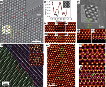
As shown in Fig. 4(a), two atomic layers of closed-packed sulfur atoms are separated by one close-packed Mo atomic layer in a single layer MoS2, which imparts its defects structures with more complexity than those in graphene or h-BN. In theory, the displacement energy for sulfur atoms in the bottom layer is approximately 6.9 eV, which indicates that the corresponding threshold energy is 90 kV. Reference Komsa, Kotakoski, Kurasch, Lehtinen, Kaiser and Krasheninnikov32 Therefore, 80 keV electron beam imaging cannot generate single-sulfur vacancy in MoS2. For sulfur atoms at the top layer, the displacement energy even exceeds 8.1 eV, Reference Komsa, Kotakoski, Kurasch, Lehtinen, Kaiser and Krasheninnikov32 which results in prominent formation of single-sulfur vacancies in comparison with double-sulfur vacancies. However, continuous 80 keV electron irradiation can eventually induce the sputtering of sulfur atoms and create sulfur vacancies in MoS2. Reference Komsa, Kotakoski, Kurasch, Lehtinen, Kaiser and Krasheninnikov32 Sulfur vacancy can be distinguished by analyzing the intensity profile. Reference Qiu, Xu, Wang, Ren, Nan, Ni, Chen, Yuan, Miao, Song, Long, Shi, Sun, Wang and Wang39 Figure 4(b) shows the comparison between intensity profiles along the lattice with (red symbol) and without (black symbol) single-sulfur vacancy, which quantitatively correspond to the simulated HRTEM image (red solid line). Reference Qiu, Xu, Wang, Ren, Nan, Ni, Chen, Yuan, Miao, Song, Long, Shi, Sun, Wang and Wang39 Under continuous electron irradiation, the sulfur vacancies tend to migrate and agglomerate to form line defects. Reference Komsa, Kurasch, Lehtinen, Kaiser and Krasheninnikov38
(a) AC–TEM image of the atomic structures of a single-layer MoS2. Red arrows indicate sulfur vacancies. Upper inset shows the edge of a single-layer MoS2. Lower inset shows the schematics of the highlighted region. Blue and yellow dots represent Mo and S atoms, respectively. (b) Intensity profile along lattices with (red symbol) and without (black symbol) sulfur vacancy, along with simulations of a single-sulfur vacancy (red line). The corresponding sections are highlighted in (a) by dashed lines. Inset shows the simulated TEM image of a single sulfur vacancy. (c–h) STEM–ADF images of six different defect configurations in MoS2. (i) AC–TEM images of MoS2 edge structure terminated with Mo atom. (j) STEM–ADF image of regular Mo-terminated edge. (k) STEM–ADF image of reconstruction of the Mo-terminated edge with the overlaid structural model. (l) STEM–ADF image of a MoS2 grain boundary. Insets are the zoom-in views of common dislocations highlighted by the blue and red rectangles. Purple and yellow circles are Mo and S2 columns, respectively. (m) STEM–ADF images of an 18.5° grain boundary consisting of dislocations with pentagon and heptagon and dislocations with hexagon and octagon. (n) STEM–ADF image of the 4|4P 60°-grain boundary structure with the overlaid structural model. (o) STEM–ADF image and overlaid structural model of a 4|4E 60°-grain boundary. The grain boundary steps are linked by 4-fold coordinated Mo atoms as highlighted. (a and b) Reprinted with permission from Ref. Reference Qiu, Xu, Wang, Ren, Nan, Ni, Chen, Yuan, Miao, Song, Long, Shi, Sun, Wang and Wang39, Copyright 2013, Macmillan Publishers Limited. (c–h, j–k, and m–o) Reprinted with permission from Ref. Reference Zhou, Zou, Najmaei, Liu, Shi, Kong, Lou, Ajayan, Yakobson and Idrobo83, Copyright 2013, American Chemical Society. (i) Reprinted with permission from Ref. Reference Komsa, Kotakoski, Kurasch, Lehtinen, Kaiser and Krasheninnikov32, Copyright 2012 American Physical Society. (l) Reprinted with permission from Ref. Reference Najmaei, Liu, Zhou, Zou, Shi, Lei, Yakobson, Idrobo, Ajayan and Lou26, Copyright 2013, Macmillan Publishers Limited.

Zhou et al. Reference Zhou, Zou, Najmaei, Liu, Shi, Kong, Lou, Ajayan, Yakobson and Idrobo83 systematically investigated the defects in CVD grown monolayer MoS2 by utilizing ADF imaging on aberration-corrected STEM. The image intensity of STEM–ADF is directly related to the atomic number, which allows unambiguous atom-by-atom chemical identification. The research group observed six different configurations of defects in MoS2, namely, single-sulfur vacancy, double-sulfur vacancy, Mo vacancy complex of Mo and nearby three sulfur atoms, vacancy complex of Mo and nearby three disulfur pairs, anti-site defects where a Mo atom substitutes for a disulfur column, and those where a disulfur column substitutes for a Mo atom, as shown in Figs. 4(c)–4(h). Reference Zhou, Zou, Najmaei, Liu, Shi, Kong, Lou, Ajayan, Yakobson and Idrobo83 Due to the lowest formation energy of all defects, single-sulfur vacancies were found considerably more frequently than double-sulfur vacancies, which is quite different from graphene for DVs are energetically more stable. Reference Zhou, Zou, Najmaei, Liu, Shi, Kong, Lou, Ajayan, Yakobson and Idrobo83,Reference Lee, Wang, Yoon, Hwang, Kim and Ho84
Under continuous electron irradiation, a crack is formed in the MoS2 membrane with the edge of Mo-terminated, as illustrated in Figs. 4(i). Reference Komsa, Kotakoski, Kurasch, Lehtinen, Kaiser and Krasheninnikov32 In addition to the regular Mo-terminated edge [Fig. 4(j)], a new type of edge reconstruction [Fig. 4(k)] is discovered, in which the outmost row of Mo atoms move closer to the inner Mo row, and the sulfur atoms at this reconstructed edge are monosulfur rather than disulfur. Reference Zhou, Zou, Najmaei, Liu, Shi, Kong, Lou, Ajayan, Yakobson and Idrobo83
Similar to grain boundaries in graphene, pentagon–heptagon dislocation cores are found in MoS2. As shown in Fig. 4(l), the pentagon and heptagon rings are Mo-oriented (blue rectangle labeled) or with sulfur substituted one of the Mo sites (red rectangle labeled). Reference Najmaei, Liu, Zhou, Zou, Shi, Lei, Yakobson, Idrobo, Ajayan and Lou26 The common pentagon–heptagon dislocations along the grain boundaries were also observed by Zhou et al., Reference Zhou, Zou, Najmaei, Liu, Shi, Kong, Lou, Ajayan, Yakobson and Idrobo83 which easily transferred to hexagon–octagon dislocations by incorporating monosulfur or disulfur into Mo–Mo bonds under sulfur-rich conditions [Fig. 4(m)]. Furthermore, the group explored several exceptional grain boundaries in MoS2 that were distinctly different from those in graphene. Figure 4(n) shows 4|4P type grain boundary, where the sulfur atoms at the grain boundary are bonded to four Mo atoms rather than three, whereas Mo atoms retain the regular 6-fold coordination. Another 4|4E type grain boundary is illustrated in Fig. 4(o); the two grains shifted laterally by half of a lattice constant along the grain boundary. The Mo atoms at the grain boundary are linked with four sulfur sites and the disulfur sites are substituted with monosulfur atom.
The in-depth atomic scale studies of structure and defects in MoS2 offer new opportunities for understanding structure–property relationship and future controlling the grain growth of MoS2.
Other 2D TMDs such as WS2 Reference Berkdemir, Gutierrez, Botello-Mendez, Perea-Lopez, Elias, Chia, Wang, Crespi, Lopez-Urias, Charlier, Terrones and Terrones27 and MoSe2 Reference Lehtinen, Kurasch, Krasheninnikov and Kaiser13 have emerged and generated substantial interest because of their specific properties. However, the in situ investigation of their structures, defects and properties is at the beginning stage, and considerable work still needs to be carried out.
III. IN SITU GROWTH OF 2D MATERIALS
Various techniques can be used to produce suitable graphene and other 2D materials layers, such as mechanical exfoliation, liquid-phase exfoliation, CVD, and molecular beam epitaxy. All these methods have their own advantages and disadvantages. A profound insight into the mechanism of nucleation and growth of 2D materials in real time by TEM is important so that we can precisely control the growth process and produce the desired materials. In situ growth of carbon nanotubes has already been investigated for decades. However, few experiments Reference Westenfelder, Meyer, Biskupek, Kurasch, Scholz, Krill and Kaiser75,Reference Rodriguez-Manzo, Pham-Huu and Banhart85–Reference Ben Romdhane, Björkman, Krasheninnikov and Banhart91 have been conducted to study the growth mechanism of 2D materials because of the difficulty in introducing source materials into high-vacuum TEM.
A. In situ growth of graphene
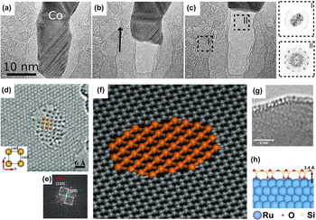
For most studies, graphene is grown by metal-catalyzed solid-state transformation of carbon at elevated temperatures. Rodriguez–Manzo et al. Reference Rodriguez-Manzo, Pham-Huu and Banhart85 deposited thin polycrystalline layers of Fe, Co, and Ni onto amorphous carbon film and increased the temperature to above 600 °C. The metal crystals began to migrate to grow thin metal layers under electron irradiation or to coalesce to form metal islands at high temperatures over the amorphous carbon films. Subsequently, the amorphous carbon films under the metal layers were dissolved, and graphene sheets began to nuclear and grow. At sufficiently high temperature, they observed the graphene by tracing the retraction of metal crystal, as shown in Figs. 5(a)–5(c). The same phenomenon was reported by He et al. Reference He, Xu, Sun, Yin, Xie, Ding, Xiu and Sun86 whose observations showed graphene sheets formed by utilizing Joule heating under a large bias voltage to extract Ag nanowire covered with thin amorphous carbon sheath. Westenfelder et al. Reference Westenfelder, Meyer, Biskupek, Kurasch, Scholz, Krill and Kaiser75 used graphene as substrate and Au as catalyst to study the in situ Joule heating-induced evolution of hydrocarbons by passing an electrical current through the substrate. The adsorbed hydrocarbons on top of graphene transformed to atomic monolayer amorphous carbon at around 1000 K and terminated in a completely polycrystalline graphene at temperature exceeding 2000 K.
(a–c) Transformation from amorphous carbon to graphene by tracing the retracting metal lamella. Insets are the diffractograms of the amorphous surrounding film and the graphene layer. Reprinted with permission from Ref. Reference Rodriguez-Manzo, Pham-Huu and Banhart85, Copyright 2011, American Chemical Society. (d) AC–TEM image of a monoatomic Fe layer with a square unit cell. Inset highlights the interatomic spacing of the square unit cell. (e) Fast Fourier transform of the structure in (d) that shows the lattice relationship between the graphene (red) and the monoatomic Fe layer (white). (f) Schematic models of a suspended monoatomic Fe layer in the graphene pore. Reprinted with permission from Ref. Reference Zhao, Deng, Bachmatiuk, Sandeep, Popov, Eckert and Ruemmeli89, Copyright 2014, American Association for the Advancement of Science. (g) Side view of the SiO2 cellular structure on Fe at 470 °C. The height of the cells is approximately 0.4 nm. (h) Schematic models of a SiO2 structure on Ru. Reprinted with permission from Ref. Reference Romdhane, Bjoerkman, Rodriguez-Manzo, Cretu, Krasheninnikov and Banhart90, Copyright 2013, American Chemical Society.

Furthermore, Liu et al. Reference Liu, Lin, Lu, Yeh, Chiu, Iijima and Suenaga88 observed the in situ in-plane growth of graphene at the step-edge of a bilayer graphene substrate, and traced the motion of Si atoms catalyst during graphene growth at the atomic scale using STEM operated at 60 kV. The growth of graphene occurred at 500–700 °C under electron irradiation, with residual hydrocarbons in the imperfect vacuum being used as the carbon source. Si atoms, which acted like catalytic active sites, slid over the graphene edges and were usually pushed to the outermost edges for further growth, or in some cases trapped by defects. They demonstrated that growth orientation was strongly affected by the step-edge structure, and growth speed depended on residual hydrocarbon gas pressure.
B. In situ growth of other 2D materials
The existence of a free-standing crystalline single-atom-thick layer of Fe was demonstrated by Zhao et al. Reference Zhao, Deng, Bachmatiuk, Sandeep, Popov, Eckert and Ruemmeli89 The group used aberration-corrected TEM investigate the structure of 2D Fe membrane, which possessed a square lattice with a 2.65 Å lattice constant at room temperature, as illustrated in Figs. 5(d)–5(f). The holes in graphene were extended to enable Fe atoms and clusters to move into and form a 2D Fe layer. The lattice of Fe layer matched better with armchair edges than zigzag edges in graphene.
Romdhane et al. Reference Romdhane, Bjoerkman, Rodriguez-Manzo, Cretu, Krasheninnikov and Banhart90,Reference Ben Romdhane, Björkman, Krasheninnikov and Banhart91 monitored the nucleation and growth of crystalline hexagonally ordered silicon oxide (SiO2) layers on transition metal surface, such as Fe, ruthenium (Ru), and cobalt (Co) with thickness of 10 nm by in situ TEM [Figs. 5(g) and 5(h)]. The nucleation of silicon oxide often begins at the surface steps Reference Ben Romdhane, Björkman, Krasheninnikov and Banhart91 or the intersection of planar defects with the metal surface at temperature values above 350 °C. Reference Romdhane, Bjoerkman, Rodriguez-Manzo, Cretu, Krasheninnikov and Banhart90 The structural defects in silica possessed the same geometry as polygons from tetragon to nonagon as reconstructed vacancies in graphene layers. Reference Romdhane, Bjoerkman, Rodriguez-Manzo, Cretu, Krasheninnikov and Banhart90
Overall, more detailed investigation into the growth mechanism of 2D materials, such as BN, MoS2, and WS2, by in situ TEM, is necessary. The results will help us precisely control the growth of 2D materials for fabrication high-quality materials and tailor them with desired properties for specific applications.
IV. IN SITU NANOFABRICATION
With the rapid development of modern TEM technology, the electron beam can be focused on spots of less than 1 Å in diameter to manipulate and engineer 2D materials at the atomic scale, instead of being used exclusively for imaging. The atoms of 2D materials in specific regions will be sputtered by the focused beam, during which the electron energy is higher than the threshold energy for atomic displacement. Nanofabrication strongly depended on the irradiation time and beam conditions, including beam size, brightness, and electron energy.
A. Doped 2D materials
Functionalized 2D materials are doped to tailor their properties for dedicated applications, including gas sensors, superconductors, supercapacitors, nanoelectronics, and spintronics. We can use the focused electron beam in TEM to create atomic-scale defects and fill these defects with the required dopants.
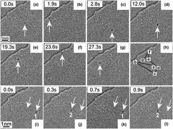
Different elements including Pt, Reference Wang, Wang, Cheng, Li, Yao, Zhang, Dong, Wang, Schwingenschloegl, Yang and Zhang58,Reference Gan, Sun and Banhart92,Reference Wang, Li, Cheng, Wang, Yao, Schwingenschlogl, Zhang and Yang93 Co, Reference Wang, Wang, Cheng, Li, Yao, Zhang, Dong, Wang, Schwingenschloegl, Yang and Zhang58 Au, Reference Gan, Sun and Banhart92,Reference Wang, Li, Cheng, Wang, Yao, Schwingenschlogl, Zhang and Yang93 Mo, Reference Rodriguez-Manzo, Cretu and Banhart94 W, Reference Cretu, Krasheninnikov, Rodriguez-Manzo, Sun, Nieminen and Banhart95 Fe, Reference Robertson, Montanari, He, Kim, Allen, Wu, Olivier, Neethling, Harrison, Kirkland and Warner57,Reference He, He, Robertson, Kirkland, Kim, Ihm, Yoon, Lee and Warner96 and Si, Reference Zhou, Kapetanakis, Prange, Pantelides, Pennycook and Idrobo97,Reference Lee, Zhou, Pennycook, Idrobo and Pantelides98 have been successfully doped in graphene by in situ TEM. Foreign atoms rapidly diffuse under electron irradiation and can be trapped in beam-induced vacancies. Most foreign atoms are located slightly outwards from the graphene layer because of the larger atomic radii of these atoms. Reference Krasheninnikov, Lehtinen, Foster, Pyykko and Nieminen99 The high binding energy between carbon and foreign atoms ensures the stability of vacancy-dopant complexes, and foreign atoms are difficult to be removed by thermal excitation or electron irradiation. Reference Wang, Wang, Cheng, Li, Yao, Zhang, Dong, Wang, Schwingenschloegl, Yang and Zhang58,Reference Gan, Sun and Banhart92,Reference Rodriguez-Manzo, Cretu and Banhart94 Nevertheless, reconstructed defects with pentagonal, heptagonal or larger rings acting as trapping centers present lower binding energy and may result in detrapping Reference Rodriguez-Manzo, Cretu and Banhart94 and migration Reference Gan, Sun and Banhart92,Reference Cretu, Krasheninnikov, Rodriguez-Manzo, Sun, Nieminen and Banhart95 of foreign atoms at high temperatures levels or high beam current densities. Figures 6(a)–6(h) show long-distance jumps of a W atom on a few-layer graphene sheet at 470 °C and an electron-beam current density of 110 A/cm2. Reference Cretu, Krasheninnikov, Rodriguez-Manzo, Sun, Nieminen and Banhart95 A W atom oscillates between two reconstructed defects with a distance of 0.5–1.4 nm, as shown in Figs. 6(i)–6(l). The strain field around reconstructed defects can result in attraction between defect and adatom. Reference Cretu, Krasheninnikov, Rodriguez-Manzo, Sun, Nieminen and Banhart95
(a–g) W atom migration (arrowed) on a few-layer graphene sheet at 470 °C. (h) Entire path from (a) to (g). (i–l) Back-and-forth jumping of a W atom between two trapping centers, 1 and 2 (arrowed). Reprinted with permission from Ref. Reference Cretu, Krasheninnikov, Rodriguez-Manzo, Sun, Nieminen and Banhart95, Copyright 2010, American Physical Society.

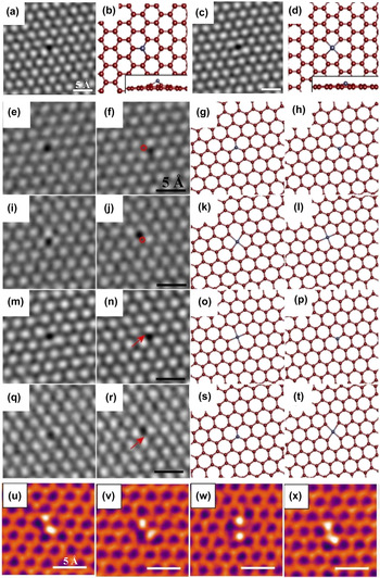
A Fe atom can occupy a MV in the graphene sheet as substitutional impurity or replace two carbon atoms in a DV as interstitial impurity, as shown in Figs. 7(a)–7(d). Reference Robertson, Montanari, He, Kim, Allen, Wu, Olivier, Neethling, Harrison, Kirkland and Warner57 The Fe atoms that occupied MV and DV are expected to possess high stability because of the high binding energy between carbon and metal atoms mentioned above. However, as revealed in Figs. 7(e)–7(t), Fe atoms can migrate under electron irradiation, the reason may be the instability of carbon atoms surrounding the Fe atom under electron irradiation, which indirectly induce the perturbation of Fe. Reference Robertson, Montanari, He, Kim, Allen, Wu, Olivier, Neethling, Harrison, Kirkland and Warner57 In details, Figs. 7(e)–7(h) show a Fe atom shifts between adjacent MV sites; Figs. 7(i)–7(l) show a Fe rotation through a change in the DV sites, whereas Figs. 7(m)–7(p) to Figs. 7(q)–7(t) illustrate a Fe atom switching between MV and DV sites. Furthermore, under continuous electron irradiation, the single Fe dopant will also be active and attract a second Fe atom to be trapped to form a Fe dimer. Reference He, He, Robertson, Kirkland, Kim, Ihm, Yoon, Lee and Warner96 As shown in Figs. 7(u)–7(x), the four different stable structures are as follows: two variants of Fe dimer in a graphene trivacancy, an Fe dimer embedded in two adjacent MVs, and an Fe dimer trapped in a tetravacancy. Reference He, He, Robertson, Kirkland, Kim, Ihm, Yoon, Lee and Warner96 Not only single or double foreign atoms can be captured by a graphene nanopore, but also atom clusters, such as Si6, as demonstrated by Lee et al. Reference Lee, Zhou, Pennycook, Idrobo and Pantelides98
Smoothed AC–TEM image of (a) an Fe substitutional defect in a graphene MV and (c) an Fe interstitial defect occupying a DV, (b) and (d) are the corresponding atomic models (the inset shows a side view). (e–t) AC–TEM images of defective Fe atom mobility and corresponding atomic models. (e and f) Shifting between adjacent MV sites, (g and h) atomic models. (i and j) Changing between two DV sites, (k and l) atomic models. (m and n) Switching from a DV to an MV site, (o and p) atomic models. (q and r) Moving from an MV to a DV site, (s and t) atomic models. Red annotations (circles or arrows) show the location of the defective atom in the previous frame. The accompanying atomic models show the Fe adatom in blue. Reprinted with permission from Ref. Reference Robertson, Montanari, He, Kim, Allen, Wu, Olivier, Neethling, Harrison, Kirkland and Warner57, Copyright 2013, American Chemical Society. (u–x) Smoothed AC–TEM images of Fe dimers in graphene vacancies. A pair of Fe atoms in (u) trivacancy, (v) alternative trivacancy, (w) tetravacancy, and (x) two adjacent monovacancies. Reprinted with permission from Ref. Reference He, He, Robertson, Kirkland, Kim, Ihm, Yoon, Lee and Warner96, Copyright 2014, American Chemical Society.

Compared with the stable vacancy-dopant complex in lattice, graphene edge can act as trapping sites for single atom as well as exhibit a rich dynamic behavior. Reference Wang, Li, Cheng, Wang, Yao, Schwingenschlogl, Zhang and Yang93,Reference Wang, Santos, Jiang, Cubuk, Ophus, Centeno, Pesquera, Zurutuza, Ciston, Westervelt and Kaxiras100 Wang et al. Reference Wang, Li, Cheng, Wang, Yao, Schwingenschlogl, Zhang and Yang93 observed an Au atom migration along the graphene edge via TEM operated at 60 kV. Notably, the trapping and detrapping processes of Au are cooperative motions with surrounding carbon atoms, especially those with unsaturated bonds. Reference Wang, Li, Cheng, Wang, Yao, Schwingenschlogl, Zhang and Yang93 The trapped atom at the edge can provide a catalytic sites for the carbon atom dissociation from graphene, whereas the trapped atom itself is intact. Reference Wang, Santos, Jiang, Cubuk, Ophus, Centeno, Pesquera, Zurutuza, Ciston, Westervelt and Kaxiras100 Wang et al. Reference Wang, Santos, Jiang, Cubuk, Ophus, Centeno, Pesquera, Zurutuza, Ciston, Westervelt and Kaxiras100 found that the Si adatom lowers the binding energy of surrounding carbon atoms and eases their removal from graphene edges under electron irradiation.
Electron-beam-induced doping can be applied in carbon atoms substitution of boron and nitrogen in h-BN to tune the electrical and magnetic properties of h-BN with different carbon content. Reference Wei, Wang, Bando and Golberg101 Wei et al. Reference Wei, Wang, Bando and Golberg101 put a paraffin wax several millimeters away from h-BN on the TEM grid as a carbon feedstock, the boron and nitrogen atoms were sputtered by electron beam (acceleration voltage at 300 kV) and left vacancies, which acted as attractive sites for carbon atoms to incorporation. They successfully transformed h-BN from electrical insulators to conductors through carbon substitutions. Reference Wei, Wang, Bando and Golberg101 In theory, the physical properties of MoS2 and other TMDs can also be modified by doping different foreign atoms. Reference Komsa, Kotakoski, Kurasch, Lehtinen, Kaiser and Krasheninnikov32,Reference Zhou, Zou, Najmaei, Liu, Shi, Kong, Lou, Ajayan, Yakobson and Idrobo83 The filling of the electron beam-induced vacancies in MoS2 was demonstrated to be feasible, but the impurity type cannot be easily identified by TEM. Reference Komsa, Kotakoski, Kurasch, Lehtinen, Kaiser and Krasheninnikov32 Therefore, further investigations on doped 2D materials and how foreign atoms tune their properties are needed to carry out.
Electron beam-induced doping is a well-controlled and simple strategy, as well as can cause less damage and can be performed at room temperature. Given these characteristics, different 2D material defects can be patterned through an electron beam and subsequently trapped or assembled foreign atoms of specific sizes or properties inside them, which may potentially lead to practical applications in the future.
B. Nanopores
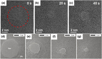
Solid-state nanopores embedded in a thin membrane open up a new field of nanosensors for their small response time and single molecule precision of characterization of chemicals and biomolecules, which may especially have revolutionary impacts on realizing single molecular gene sequencing. Reference Storm, Chen, Ling, Zandbergen and Dekker102,Reference Xu, Yin, Xie, He, Wang and Sun103 The focused electron beam can be used to fabricate nanopores in silicon nitride, Reference Kim, McNally, Murata and Meller104 silicon oxide, Reference Storm, Chen, Ling, Zandbergen and Dekker102 graphene Reference Xu, Yin, Xie, He, Wang and Sun103,Reference Xu, Xie, Yin, Sun, He and Sun105 and magnesium (Mg) Reference Wu, Cao, Zheng, Sheng, Liu, Liu, Zhao and Wang106,Reference Zheng, Liu, Cao, Wu, Jia, Cao, Zhao and Wang107 in TEM. However, electron beam does not give full control over the nanopores at the nanometer scale because no images can be recorded during drilling. Nanopore size and crystallinity can be further fine-tuned by electron irradiation Reference Storm, Chen, Ling, Zandbergen and Dekker102,Reference Wu, Cao, Zheng, Sheng, Liu, Liu, Zhao and Wang106,Reference Zheng, Liu, Cao, Wu, Jia, Cao, Zhao and Wang107 and in situ thermal heating. Reference Xu, Yin, Xie, He, Wang and Sun103,Reference Song, Schneider, Xu, Pandraud, Dekker and Zandbergen108 Nanopore sizes have been demonstrated to be reduced or increased to find a configuration with the lowest surface-free energy. Whether the nanopores expand or shrink depends on the relationship between sheet thickness and nanopore diameter. Reference Storm, Chen, Ling, Zandbergen and Dekker102,Reference Xu, Yin, Xie, He, Wang and Sun103 In detail, the nanopores with diameter smaller than thickness will lower the surface-free energy by reducing size, whereas the nanopores with diameter larger than thickness will do so by increasing size. Reference Storm, Chen, Ling, Zandbergen and Dekker102 The contraction rate of the nanopores is inversely proportional to the membrane thickness; when the membrane is thinner, the contraction rate is larger. Reference Kim, McNally, Murata and Meller104
Figures 8(a)–8(c) illustrate the electron beam induced nanofabrication on a graphene membrane. Figure 8(a) is the pristine graphene membrane before high dose irradiation. After long time exposure to electron beam, the region highlighted by dashed rings transformed into amorphous carbon in Fig. 8(b) and eventually formed a nanopore in Fig. 8(c). The graphene nanopores open up new avenues for the single-base resolution on DNA because the distance between adjacent base pairs on stretched DNA (0.36 nm) matches well with the single-layer graphene thickness (0.34 nm). Reference Xu, Yin, Xie, He, Wang and Sun103 As shown in Figs. 8(d)–8(g), electron irradiation induced the silicon oxide nanopore to gradually shrink from 19 to about 3 nm. Reference Storm, Chen, Ling, Zandbergen and Dekker102
(a–c) Nanopore fabrication in the graphene sheet. (a) Pristine graphene membrane before high-dose irradiation. The dashed ring highlights the region to be irradiated. (b–c) The same region in (a) after electron beam irradiation for 20 and 48 s and eventually forming a graphene nanopore. Reprinted with permission from Ref. Reference Xu, Xie, Yin, Sun, He and Sun105, Copyright 2014, Wiley–VCH Verlag GmbH & Co. KGaA, Weinheim. (d–g) The shrinkage process of a SiO2 nanopore from a size of 19 to about 3 nm under electron beam irradiation. Reprinted with permission from Ref. Reference Storm, Chen, Ling, Zandbergen and Dekker102, Copyright 2003, Nature Publishing Group.

Furthermore, the nanopores can also nucleate at contamination sites Reference Meyer, Eder, Kurasch, Skakalova, Kotakoski, Park, Roth, Chuvilin, Eyhusen, Benner, Krasheninnikov and Kaiser47 or surrounding vacancies Reference Krasheninnikov and Banhart109 without the focused electron beam.
C. Nanoribbons
Under electron irradiation, the two adjacent graphene nanopores are continuously growing and the bridges between them narrowed to nanoribbons. Reference Song, Schneider, Xu, Pandraud, Dekker and Zandbergen108,Reference Chuvilin, Meyer, Algara-Siller and Kaiser110–Reference Fischbein and Drndić112 Graphene nanoribbons open up a band gap in graphene and can exhibit either quasimetallic or semiconducting behavior, which highly relies on the edge structure. Reference Jia, Hofmann, Meunier, Sumpter, Campos-Delgado, Romo-Herrera, Son, Hsieh, Reina, Kong, Terrones and Dresselhaus113 For instance, the graphene nanoribbons with a higher zigzag edge fraction exhibited a smaller energy gap than predominant armchair nanoribbons of similar width. Reference Ritter and Lyding114 Therefore, controlling the configuration and crystallinity of the edge structures is important to tailor the properties of nanoribbons. Jia et al. Reference Jia, Hofmann, Meunier, Sumpter, Campos-Delgado, Romo-Herrera, Son, Hsieh, Reina, Kong, Terrones and Dresselhaus113 produced atomically smooth and highly crystalline zigzag or armchair edges from defective nanoribbon edges by using Joule heating and electron irradiation.
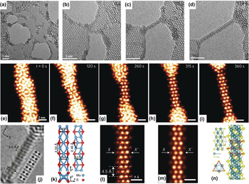
When the graphene nanoribbon width is reduced below 1 nm, it reconstructs from the hexagonal structure to intermediate structures with pentagons and heptagons. Reference Chuvilin, Meyer, Algara-Siller and Kaiser110 Eventually, the graphene nanoribbons convert to one or two atomic carbon chains. Reference Song, Schneider, Xu, Pandraud, Dekker and Zandbergen108,Reference Chuvilin, Meyer, Algara-Siller and Kaiser110,Reference Jin, Lan, Peng, Suenaga and Iijima111 The double chains are generally shorter than the single carbon chains, whereas the single chains frequently change their anchor sites. Reference Song, Schneider, Xu, Pandraud, Dekker and Zandbergen108,Reference Jin, Lan, Peng, Suenaga and Iijima111 The thinning process is dominated by a surface atom sputtering mechanism, in which the atoms at the edges are preferred to be removed. Reference Jin, Lan, Peng, Suenaga and Iijima111 Moreover, monoatomic carbon chains could be fabricated from graphene nanoribbons through loading a bias by Cretu et al., Reference Cretu, Botello-Mendez, Janowska, Cuong, Charlier and Banhart115 and they measured the in situ electrical properties and found that the electrical conductivity of atomic carbon chains is lower than predicted ideal chains. For TMDs, such as MoS2, MoSe2, WS2, and WSe2, the nanoribbons with sub-nanometer width can be widely formed between holes created by manipulating a focused electron beam. Reference Lin, Cretu, Zhou, Suenaga, Prasai, Bolotin, Cuong, Otani, Okada, Lupini, Idrobo, Caudel, Burger, Ghimire, Yan, Mandrus, Pennycook and Pantelides16,Reference Liu, Xu, Wu, Zhang, Yu, Qiu, Hong, Jin, Li, Wang, Sun and Guo17 Liu et al. Reference Liu, Xu, Wu, Zhang, Yu, Qiu, Hong, Jin, Li, Wang, Sun and Guo17 combined the in situ HRTEM characterization with first-principle calculations and demonstrated the sub–1 nm ribbon as a Mo5S4 crystal with a band gap of 0.77 eV, which indicates the nanoribbon is semiconducting [Figs. 9(a)–9(f)]. On the other hand, Lin et al. Reference Lin, Cretu, Zhou, Suenaga, Prasai, Bolotin, Cuong, Otani, Okada, Lupini, Idrobo, Caudel, Burger, Ghimire, Yan, Mandrus, Pennycook and Pantelides16 gave a more detailed investigation of nanoribbon structure and property through STEM and in situ electrical measurement. The nanoribbons with stoichiometry MS (M = Mo or W, X = S or Se) matched better with the experimental results and were demonstrated to be metallic [Figs. 9(g)–9(n)]. The nanoribbons are mechanically robust and have high crystalline perfection, Reference Lin, Cretu, Zhou, Suenaga, Prasai, Bolotin, Cuong, Otani, Okada, Lupini, Idrobo, Caudel, Burger, Ghimire, Yan, Mandrus, Pennycook and Pantelides16,Reference Liu, Xu, Wu, Zhang, Yu, Qiu, Hong, Jin, Li, Wang, Sun and Guo17 which may serve as interconnects in future flexible nanocircuits.
(a–d) TEM images of Mo5S4 nanoribbon formation. The bridge between two adjacent nanopores narrowed to nanoribbons with nanopore expansion. (e–i) False-colored STEM images of the MoSe nanoribbon formation. (j) HRTEM image and simulated TEM image (labeled by the dotted rectangle) of Mo5S4. (k) Three-view depictions of the Mo5S4 nanoribbon. (l) STEM image and (m) simulated STEM image of MoSe nanoribbon. (n) Atomic structural model of the MS (M = Mo or W, X = S or Se) nanoribbon. (a–d and j–k) Reprinted with permission from Ref. Reference Liu, Xu, Wu, Zhang, Yu, Qiu, Hong, Jin, Li, Wang, Sun and Guo17, Copyright 2013, Macmillan Publishers Limited. (e–i and l–n) Reprinted with permission from Ref. Reference Lin, Cretu, Zhou, Suenaga, Prasai, Bolotin, Cuong, Otani, Okada, Lupini, Idrobo, Caudel, Burger, Ghimire, Yan, Mandrus, Pennycook and Pantelides16, Copyright 2014, Macmillan Publishers Limited.

The approach in sculpting 2D materials into nanopores, nanoribbons, and nanochains by electron irradiation could be developed into a general controllable method for ultrasmall component fabrication for future functional devices.
V. IN SITU PROPERTY CHARACTERIZATION
Given a clear understanding of 2D material structures at atomic resolution, introducing external fields, such as electron irradiation, thermal excitation, electrical field, and mechanical force, into TEM is significant in the investigation of essential structural evolution and structure–property relationship of 2D materials in real environment. Various external stimuli can be recognized through different specimen holders.
A. Electron irradiation
Electron irradiation is inevitable and can be easily recognized in TEM. A virtue can be made out of necessity, and electron irradiation can not only induce in situ growth and nanofabrication of 2D materials by using high temperature, as discussed above, but also induce structural evolution such as production, Reference Meyer, Kisielowski, Erni, Rossell, Crommie and Zettl14,Reference Robertson, Allen, Wu, He, Olivier, Neethling, Kirkland and Warner24,Reference Robertson and Warner48 migration, Reference Kotakoski, Mangler and Meyer49 reconstruction, and annihilation Reference Meyer, Kisielowski, Erni, Rossell, Crommie and Zettl14,Reference Robertson, Allen, Wu, He, Olivier, Neethling, Kirkland and Warner24 of defects. Modern HRTEM with ultrafast imaging technology makes it possible to record the dynamic process of structural evolution in real time, which leads us to a new understanding of electron irradiation effects in 2D materials.
Robertson et al. Reference Robertson, Allen, Wu, He, Olivier, Neethling, Kirkland and Warner24 utilized the focused electron beam to generate defects in graphene layers, and investigated how the beam current density and exposure time influence the complexity of defects. They found that defects were created in a clean area (∼10 × 10 nm2) of pristine graphene only when the beam current density reached ∼108 e/m2 s1, and increasing the exposure time (up to 120 s) to the focused beam gave rise to further complex defects.
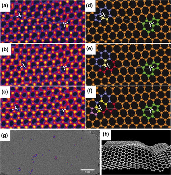
The full life cycle of a dislocation from generation, migration, interaction with other dislocations to eventual annihilation under electron irradiation has been recorded by Lehtinen et al. Reference Lehtinen, Kurasch, Krasheninnikov and Kaiser13 At first, carbon atoms were sputtered by electron beam and formed vacancies in graphene, and the vacancies agglomerated and reconstructed into a dislocation under continuous electron irradiation. Reference Cretu, Botello-Mendez, Janowska, Cuong, Charlier and Banhart115 Subsequently, the dislocation migrated within the graphene sheet through bond rotations along the glide plane (glide) and two carbon atom addition or removal (climb) in different directions. Reference Cretu, Botello-Mendez, Janowska, Cuong, Charlier and Banhart115 The mechanism of migration through beam-driven bond rotations was consistent with what Kotakoski et al. Reference Kotakoski, Mangler and Meyer49 found through observation of DV motion in graphene using STEM operated at 60 kV. Eventually, due to the attractive force between the dislocations and the migration induced by electron irradiation, they moved toward each other and ultimately annihilated. Reference Cretu, Botello-Mendez, Janowska, Cuong, Charlier and Banhart115 On the other hand, dislocations in graphene can generate in-plane strain Reference Warner, Margine, Mukai, Robertson, Giustino and Kirkland15 and out-of-plane distortions and ripples. Warner et al. Reference Warner, Margine, Mukai, Robertson, Giustino and Kirkland15 studied the dynamics of dislocation pairs in graphene and their impact on the lattice structure of graphene. Figures 10(a)–10(f) show the dislocations migrate along the zigzag lattice through glide and climb mechanism activated by electron beam, which was mentioned above. Reference Cretu, Botello-Mendez, Janowska, Cuong, Charlier and Banhart115 They used the geometric phase analysis to map the strain fields, and illustrated that the graphene was deformed by bond compression or elongation, shear strain and lattice rotations of dislocations. Reference Warner, Margine, Mukai, Robertson, Giustino and Kirkland15 Moreover, Warner et al. Reference Warner, Fan, Robertson, He, Yoon and Lee116 utilized a novel approach to introducing a large number of dislocations (5–7 ring pairs) in a well-defined graphene area by slowly raster-scanning a focused electron beam back and forth. To release the large strain produced by the large amount of dislocations, the graphene formed out-of-plane distortions and ripples, as shown in Figs. 10(h). Reference Warner, Fan, Robertson, He, Yoon and Lee116 The rippling was dynamic and could fluctuate between various structural configurations under electron irradiation, which was distinct from in-plane lattice compression mentioned above. Reference Warner, Margine, Mukai, Robertson, Giustino and Kirkland15
(a–c) Real-time dislocation dynamics: HRTEM images showing changes in the position of an edge glide dislocation with time under continuous electron beam irradiation. (a) Time = 0 s, (b) time = 141 s, and (c) time = 321 s. (d–f) Atomic models of (a–c), respectively. White T indicates the position of dislocation. Reprinted with permission from Ref. Reference Warner, Margine, Mukai, Robertson, Giustino and Kirkland15, Copyright 2012, American Association for the Advancement of Science. (g) TEM image of 41 dislocations [5–7 ring pairs (red−blue)] in graphene introduced by electron beam irradiation. (h) Schematic ripple morphology in graphene. Reprinted with permission from Ref. Reference Warner, Fan, Robertson, He, Yoon and Lee116, Copyright 2013, American Chemical Society.

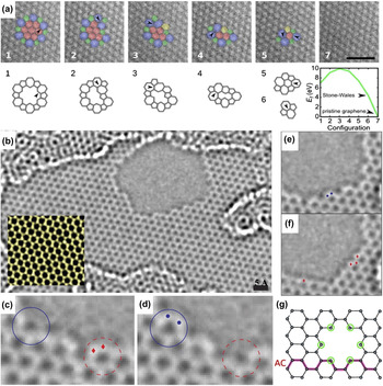
The grain boundary migration in graphene with atomic resolution has been investigated in real time by using electron irradiation-induced bond rotation in aberration-corrected TEM. Reference Kurasch, Kotakoski, Lehtinen, Skákalová, Smet, Krill, Krasheninnikov and Kaiser66 The grain boundary translation only occurs at significant high boundary curvature, which has a high driving force. Reference Kurasch, Kotakoski, Lehtinen, Skákalová, Smet, Krill, Krasheninnikov and Kaiser66 Figure 11(a) step-by-step shows how a flower-like grain boundary unwinds under electron irradiation and ultimately disappears, resulting to pristine graphene restoration. Moreover, each of the unwinding steps lowers the total system energy, and the process is irreversible.
(a) Disappearance process of a flower defect under electron beam irradiation during a 30 s total exposure, below the experimental images are DFT-optimized models of the corresponding structures above and a plot of their formation energies. Rotating bonds are indicated by black arrows. Reprinted with permission from Ref. Reference Kurasch, Kotakoski, Lehtinen, Skákalová, Smet, Krill, Krasheninnikov and Kaiser66, Copyright 2012, American Chemical Society. (b) AC–TEM image of a hole in a single layer of graphene produced by prolonged irradiation, (Inset) Averaged series of images showing the atomically resolved graphene lattice. (c–d) Hole evolution, with (d) following 4 s after (c). Two carbon atoms (red dots in the dashed circle) are removed while two nearby carbon atoms (blue dots) bind to their neighbors to close a hexagon (solid circle). (e–f) Edge reconfiguration: conversion from an armchair edge (b) to a zigzag edge (c) after 4 s. The two atoms marked as blue dots in (e) disappeared in (f), where four new carbon atoms are incorporated as red diamonds. Reprinted with permission from Ref. Reference Girit, Meyer, Erni, Rossell, Kisielowski, Yang, Park, Crommie, Cohen, Louie and Zettl10, Copyright 2009, American Association for the Advancement of Science. (g) Schematic morphology of the hole in graphene. Under-coordinated atoms, which are equally likely to be sputtered away marked with green circles. Removing any of these atoms results in zigzag edges. Reprinted with permission from Ref. Reference Kotakoski, Santos-Cottin and Krasheninnikov68, Copyright 2012, American Chemical Society.

The carbon atoms dynamics at the edge of a hole in single-layer graphene under electron irradiation is recorded by using the aberration corrected TEM equipped with a monochromator. Reference Girit, Meyer, Erni, Rossell, Kisielowski, Yang, Park, Crommie, Cohen, Louie and Zettl10 The hole formed by prolonged electron irradiation is showed in Fig. 11(b) at atomic resolution. The disappearance of two carbon atoms (red dots) and the incorporation of two atoms (blue dots), with time interval of 4 s, can be seen in Figs. 11(c) and 11(d). An armchair sequence at a corner transformed into a zigzag sequence over the course of 4 s, as shown in Figs. 11(e) and 11(f). The three main competing mechanisms that result in the dynamics of edge reconstruction and hole growth are the migration of dangling carbon atom, the ejection of carbon atom along the edge, and the addition of carbon atoms from adsorbates attached on the hole. Reference Girit, Meyer, Erni, Rossell, Kisielowski, Yang, Park, Crommie, Cohen, Louie and Zettl10
Understanding the evolution and dynamics of dislocations, grain boundaries and edge structures under electron irradiation, represents a significant step forward in realizing the goals to manipulate and modify of carbon nanomaterials by utilizing the electron beam for nanodevice fabrication in the future.
B. Thermal field
In situ heating can be realized by placing a heating element at the tip of a TEM specimen holder, and the temperature is set using an external controller. The three typical types of in situ heating TEM holders are furnace-heating holders, wire-heating holders, and membrane-heating holders. Reference Ziegler, Graafsma, Zhang and Frenken18 In furnace-heating holders, the thermal expansion effect causes a serious problem of sample drifting when changing temperature, which makes it impossible to take HRTEM images in a short period of time. Reference Ziegler, Graafsma, Zhang and Frenken18 A cooling system is required to maintain the stability of the holders because the heating area is large. The wire-heating holder can reach a temperature as high as 1500 °C and do not need cooling water, whereas the membrane-heating holder has the fastest temperature change, ranging at 106 °C/s. Reference Ziegler, Graafsma, Zhang and Frenken18 However, sample drifting cannot be avoided. An alternative approach is to use the Joule heating with small specimen drift when a bias voltage is applied to an STM or electrical bias holder. Unfortunately, the temperature induced by Joule heating cannot be directly read. All these heating methods make it feasible to study thermal properties of 2D materials as well as thermal excitation-induced behavior.
As mentioned above, at elevated temperatures, nanopores can shrink or expand, Reference Xu, Yin, Xie, He, Wang and Sun103,Reference Song, Schneider, Xu, Pandraud, Dekker and Zandbergen108 foreign atoms can be introduced into 2D materials to tune their properties, Reference Gan, Sun and Banhart92,Reference Rodriguez-Manzo, Cretu and Banhart94,Reference Cretu, Krasheninnikov, Rodriguez-Manzo, Sun, Nieminen and Banhart95 and thermal-induced in situ growth of graphene can also be realized in TEM. Reference Westenfelder, Meyer, Biskupek, Kurasch, Scholz, Krill and Kaiser75,Reference Rodriguez-Manzo, Pham-Huu and Banhart85,Reference He, Xu, Sun, Yin, Xie, Ding, Xiu and Sun86,Reference Romdhane, Bjoerkman, Rodriguez-Manzo, Cretu, Krasheninnikov and Banhart90,Reference Ben Romdhane, Björkman, Krasheninnikov and Banhart91
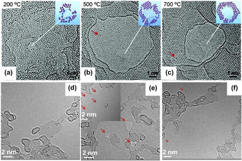
2D material defects are usually undesirable for electronic applications; thus, repairing the defects would be extremely useful. Some defects can relax to simple structures through bond rotations and surface adatom incorporations under electron irradiation. Reference Robertson, Allen, Wu, He, Olivier, Neethling, Kirkland and Warner24 However, this process may take a long time and is infeasible for large-scale graphene restoration. Fortunately, at high temperatures, the diffusing carbon adatoms can be rapidly trapped by defects, which results in self-healing and single-crystallinity recovery of graphene. Reference Song, Schneider, Xu, Pandraud, Dekker and Zandbergen108,Reference Chen, Shi, Cai, Xu, Sun, Wu and Yu117 Figures 12(a)–12(c) reveal a temperature-dependent self-healing mechanism that tunes the graphene nanopore from amorphous to single crystalline at temperature of 700 °C. Reference Song, Schneider, Xu, Pandraud, Dekker and Zandbergen108 Figures 12(d)–12(f) show HRTEM images of the three graphene samples before and after plasma treatment and after annealing. Reference He, Xu, Xu, Zeng, Xu, Sun, Wang, Xing, Wu, Lu, Liu, Chen and Chu117 After plasma treatment, a large amount of vacancies exists in graphene, which are indicated by red arrows in Fig. 12(e). As shown in Fig. 12(f), the defect density is substantially reduced after annealing at 750 °C.
(a–c) Self-repair process of the graphene nanopore from (a) amorphous to (b) polycrystalline, and ultimately to (c) single crystalline with the temperature increasing from 200 to 500 °C, and finally to 700 °C. Reprinted with permission from Ref. Reference Song, Schneider, Xu, Pandraud, Dekker and Zandbergen108, Copyright 2011, American Chemical Society. (d–f) HRTEM images of three graphene samples: (d) pristine, (e) after 5 s of plasma treatment, and (f) after annealing at 750 °C. The surfaces are partially covered by polymethyl methacrylate (PMMA) residue. Red arrows indicate honeycomb lattice vacancies. Reprinted with permission from Ref. Reference Chen, Shi, Cai, Xu, Sun, Wu and Yu117, Copyright 2013, American Institute of Physics.

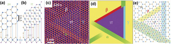
Moreover, thermal excitation can induce phase transition, Reference He, Xu, Xu, Zeng, Xu, Sun, Wang, Xing, Wu, Lu, Liu, Chen and Chu118,Reference Lin, Dumcenco, Huang and Suenaga119 as shown in Fig. 13. Monolayer MoS2 has two distinct symmetries: the semiconducting 2H (trigonal prismatic D3h) and the metallic 1T (octahedral Oh). The dynamic transformation process between 2H and 1T phases with atomic resolution was first investigated using in situ STEM by Lin et al. Reference Eda, Fujita, Yamaguchi, Voiry, Chen and Chhowalla120 Phase transformation occurred at 600 °C under continuous electron irradiation by gliding atomic planes of S and Mo. Phase transition requires an intermediate phase (α-phase) and migration of two kinds of boundaries (β- and γ-boundaries), as shown in Figs. 13(c)–13(e). The α-phase is a precursor during phase transition, which consists of 3–4 constricted MoS2 zigzag chains. Reference Lin, Dumcenco, Huang and Suenaga119 The β-boundary contains four-membered Mo–S rings, whereas the γ-boundary includes two constricted MoS2 zigzag chains. Reference Lin, Dumcenco, Huang and Suenaga119 The coexistence of the semiconducting 2H and the metallic 1T phase can form the coherent electronic heterostructures with tunable band gap, which may be exploited for novel molecular functionalities in the future. Reference Lin, Dumcenco, Huang and Suenaga119,Reference Eda, Fujita, Yamaguchi, Voiry, Chen and Chhowalla120
(a–b) Schematic models of monolayer MoS2 with 2H (a) and 1T (b) phases in basal plane and cross-section views. Mo, blue; top S, orange; bottom S′, purple. (c) STEM high angle annular dark field (STEM-HAADF) image of triangular 1T phase MoS2 embedded in 2H phase MoS2. At the edges between the 1T and 2H phase are the three different boundaries (α, β, and γ). (d) Simple schematic illustration and (e) schematic model of (c). Reprinted with permission from Ref. Reference Lin, Dumcenco, Huang and Suenaga119, Copyright 2014, Macmillan Publishers Limited.

By in situ Joule heating, graphene cracks propagate from the flake edges and result in the formation of narrow gap before breakdown. Reference Barreiro, Borrnert, Rummeli, Buchner and Vandersypen121,Reference Borrnert, Barreiro, Wolf, Katsnelson, Buchner, Vandersypen and Rummeli122 In another example, in situ Joule heating can induce the suspended few-layer graphene to sublimate, with the sublimation fronts predominantly consisted of zigzag edges. Reference Huang, Ding, Yakobson, Lu, Qi and Li123 The graphene edges reconstructed during sublimation and most frequently formed bilayer edges, indicating that bilayer edges are more stable than monolayer at high temperatures. Reference Huang, Ding, Yakobson, Lu, Qi and Li123
C. Electrical field
In situ electrical measurement is often used to study behavior and structural changes Reference Barreiro, Borrnert, Rummeli, Buchner and Vandersypen121,Reference Huang, Ding, Yakobson, Lu, Qi and Li123 of specimens in an electrical field, electrical transport properties Reference Lin, Cretu, Zhou, Suenaga, Prasai, Bolotin, Cuong, Otani, Okada, Lupini, Idrobo, Caudel, Burger, Ghimire, Yan, Mandrus, Pennycook and Pantelides16,Reference Cretu, Botello-Mendez, Janowska, Cuong, Charlier and Banhart115 of nanostructures. STM holders are popular for these application purposes. A metallic probe in the STM holder is present, which connects to the power supply unit and can move back and forth in fine steps controlled by a piezo manipulator. Reference Ziegler, Graafsma, Zhang and Frenken18 Different kinds of tips, such as W, Cu, Au, and Ag, are placed on the probe to contact the specimens. A circuit can be formed with the TEM specimen and probe for electrical current to pass through. For example, in situ electrical measurement of MoSe nanowire provides direct evidence of the conversion from semiconducting monolayer to metallic nanowire. Reference Lin, Cretu, Zhou, Suenaga, Prasai, Bolotin, Cuong, Otani, Okada, Lupini, Idrobo, Caudel, Burger, Ghimire, Yan, Mandrus, Pennycook and Pantelides16
With in situ TEM, Barreiro et al. Reference Barreiro, Borrnert, Rummeli, Buchner and Vandersypen121,Reference Borrnert, Barreiro, Wolf, Katsnelson, Buchner, Vandersypen and Rummeli122 observed how the current modified the graphene structure and vice versa. Figure 14(a) schematically shows the in situ TEM setup with a sheet of few-layered graphene linked with two free-standing gold electrodes to form a circuit. Through large bias application, few-layered suspended graphene were peeled off layer by layer until only a single layer remained. Reference Barreiro, Borrnert, Rummeli, Buchner and Vandersypen121 Subsequently, the monolayer graphene began to crack and formed a narrow constriction. Reference Borrnert, Barreiro, Wolf, Katsnelson, Buchner, Vandersypen and Rummeli122,Reference Huang, Ding, Yakobson, Lu, Qi and Li123 By real-time electrical measurement, the current through the constriction drops when the constriction width is reduced, and eventually drops to zero when the constriction fails [Fig. 14(b)]. Current drop means the resistance is increasing, which indirectly proves that the carbon atoms are sublimed under the large bias. Reference Barreiro, Borrnert, Rummeli, Buchner and Vandersypen121,Reference Borrnert, Barreiro, Wolf, Katsnelson, Buchner, Vandersypen and Rummeli122
(a) Schematic overview of the setup. (left) STEM image of the electrodes with a sketch of an overlying graphene ribbon with a central constriction. (right) TEM image of the bilayer graphene constriction at high bias. The inset is the FFT of the marked region in the micrograph. (b) Series of micrographs at high bias. The plot indicates the measured current through the constriction. The transparent bars indicate when the respective series of color-coded micrographs were taken. Reprinted with permission from Ref. Reference Borrnert, Barreiro, Wolf, Katsnelson, Buchner, Vandersypen and Rummeli122, Copyright 2012, American Chemical Society. (c–d) Electrical current through two monatomic carbon chains at a constant bias of 1 V. Blue curve shows the evolution of the current. The filled regions under the curve correspond to the periods where the chains appeared. The image insets show the respective chains. Reprinted with permission from Ref. Reference Cretu, Botello-Mendez, Janowska, Cuong, Charlier and Banhart115, Copyright 2013, American Chemical Society. (e) TEM images of a strained carbon chain and (g) corresponding current–voltage curves. (f) TEM images of an unstrained wavy carbon chain and (h) corresponding current–voltage curves. Reprinted with permission from Ref. Reference Torre, Botello-Mendez, Baaziz, Charlier and Banhart124, Copyright 2015, Macmillan Publishers Limited.

Furthermore, Lu et al. Reference Lu, Merchant, Drndic and Johnson125 found that the graphene constriction conductance was high and approximately varied with width, as G(w) = (e 2/h) w 0.75, where w is the constriction width in nanometers. When the graphene nanoconstriction is narrowed to single carbon atom chains, a characteristic drop of the electrical current occurs, as shown in Figs. 14(c) and 14(d). Reference Cretu, Botello-Mendez, Janowska, Cuong, Charlier and Banhart115 For the electrical measurements of monoatomic carbon chains, Torre et al. Reference Torre, Botello-Mendez, Baaziz, Charlier and Banhart124 found that the strained carbon chains were semiconducting with polyyne structure (–C≡C–C≡C–C≡), while unstrained chains were metallic with cumulene structure (=C=C=C=C=C=). They also observed the semiconductor–metal transition of carbon chain through a release of strain. The S-shaped current–voltage curve in Fig. 14(g) indicates the semiconducting behavior of carbon chain under strain. Reference Torre, Botello-Mendez, Baaziz, Charlier and Banhart124 Conversely, an unstrained chain is shown in Fig. 14(h), in which the current–voltage curve is a linear. Reference Torre, Botello-Mendez, Baaziz, Charlier and Banhart124
D. Mechanical force field
When the materials size decreases to the nanometer level, the mechanical properties, including strength, hardness, and toughness, may experience dramatically changes. Reference Ziegler, Graafsma, Zhang and Frenken18 Predicting and correctly understanding nanostructure failure is important, as well as the material size effect on mechanical behaviors. Reference Ziegler, Graafsma, Zhang and Frenken18 Therefore, mechanical TEM holders are designed to load a tensile or compressive mechanical force on TEM specimens and track the structural evolution simultaneously. Reference Ziegler, Graafsma, Zhang and Frenken18
The mechanical properties of CNTs, Reference Wang, Golberg and Bando126 nanocrystals, Reference Zheng, Cao, Weinberger, Huang, Du, Wang, Ma, Xia and Mao127–Reference Sun, He, Lo, Xu, Bi, Sun, Zhang, Mao and Li129 and nanowires Reference Han, Zhang, Zheng, Zhang, Zhang, Hao, Guo, Yuan and Wang130–Reference Wang, Liu, Guan, Yang, Sun, Cheng, Hirata, Zhang, Ma, Chen and Han133 have been investigated in detail by in situ mechanical techniques. However, given the nature of 2D materials, the boundary conditions are complicated and more difficult to control in in situ experiment. The mechanical properties of 2D materials are still difficult to characterize inside a TEM.
Tang et al. Reference Tang, Kvashnin, Najmaei, Bando, Kimoto, Koskinen, Ajayan, Yakobson, Sorokin, Lou and Golberg134 developed an in situ TEM probing technique to investigate the nanomechanical cleavage of 2D crystals. The MoS2 was successfully cleaved from a monolayer to double layers and up to 23 atomic layers, which demonstrated that the technique could realize layer number selective cleavage, and such cleavage is highly reversible. Reference Tang, Kvashnin, Najmaei, Bando, Kimoto, Koskinen, Ajayan, Yakobson, Sorokin, Lou and Golberg134 The MoS2 crystals were loaded on the Au stage and a W tip was controlled to cleave and bend the MoS2 atomic layers, as shown in the schematic [Fig. 15(a)] and corresponding TEM image [Fig. 15(b)]. Figures 15(c)–15(f) show the cleavage process of a monolayer MoS2. The W probe initially contacted the outermost monolayer edge and then moved at an inclined angle marked by a black arrow, which made the monolayer MoS2 attach to the probe [Fig. 15(c)]. By moving the probe away, the monolayer MoS2 flake was stretched and eventually detached from the crystal. Reference Tang, Kvashnin, Najmaei, Bando, Kimoto, Koskinen, Ajayan, Yakobson, Sorokin, Lou and Golberg134
(a) Schematic of the experimental setup and (b) corresponding TEM image. (c–f) Nanomechanical cleavage process of a monolayer MoS2: (c) the initial contact, (d) intermediate peeled-off and bent, and (e) stretched states of a monolayer MoS2. (f) HRTEM image of the cleaved monolayer MoS2, revealing the (100) atomic stacking order, as well as the MoS2 (002) lattice fringes of the “mother” crystal. Reprinted with permission from Ref. Reference Tang, Kvashnin, Najmaei, Bando, Kimoto, Koskinen, Ajayan, Yakobson, Sorokin, Lou and Golberg134, Copyright 2014, Macmillan Publishers Limited. (g) TEM image of a multilayer graphene nanosheet clamped between the atomic force microscope (AFM) and W tips. (h) TEM image of the nanosheet in (g) after a V-shaped notch was fabricated at its upper edge. (i) TEM image of the nanosheet after it was fractured from the notch tip. (j) Schematic of fracture toughness testing setup. (k) HRTEM image of the framed area in (g). (l) Force curve recorded during the nanosheet fracture testing. Reprinted with permission from Ref. Reference Wei, Xiao, Li, Tang, Chen, Bando and Golberg135, Copyright 2015, American Chemical Society.

Wei et al. Reference Wei, Xiao, Li, Tang, Chen, Bando and Golberg135 first reported the in situ fracture of single-edged V/U–notched multilayer graphene and BN in HRTEM. As shown in Fig. 15(g), a graphene nanosheet was clamped between a force-sensing cantilever (AFM tip) and a movable W tip at its upper edge. A V-shaped notch was made at the middle of the clamped edge by a 300 keV focused electron probe [Fig. 15(h)]. The W tip retracted at a constant speed to fracture the nanosheet from the V-notch tip into two pieces [Fig. 15(i)]. The tension force measured in real-time, increased linearly to 1210 nN and then abruptly dropped to zero [Fig. 15(l)].
With the assistance of in situ TEM measurements, both synthesis and property characterization can be simultaneously realized inside the TEM, which is significant in guiding 2D materials design with novel properties for future development.
VI. SUMMARY AND OUTLOOK
With the rapid development of TEM technology and specialized specimen holders, TEM is utilized not only for imaging and characterizing but also as a nanolab for materials. By introducing various external fields, such as electron irradiation, thermal excitation, electrical field, and mechanical force, into TEM, its rich potential for simulating real environment is unrivalled by any other techniques. However, there are still great inherent limitations. In situ TEM makes it feasible to monitor the dynamic process of chemical reaction and structural evolution at atomic resolution in real time and understand the essential relationship of structures and properties. Since the emerging of 2D materials with extraordinary properties, TEM will definitely have a revolutionary effect on the future development of novel materials. However, there are many inherent limitations of TEM which need to further overcome, like the small sample size, lack of supporting substrates, and difficult to simulate competitive environment. Although a large amount of in situ experiments have been carried out to investigate the structure and structure–property relationship of 2D materials, little is known about the chemistry, bonding, photonic response, and electrical and magnetic properties of TEM. Many challenges exist for the further investigation of the novel 2D materials.
For future work, improving the TEM technology is necessary to achieve ultrahigh spatial and temporal resolution so that each transient moment can be captured during the dynamic material processes. The changes in chemical components and bonding need to be recorded as well. Furthermore, in situ TEM needs to simulate more complicated environments (gas, liquid, and solid) with multiple stimuli (e.g., electromagnetic field, tunable light, and mechanical stress) and simultaneously measure multiple properties (Fig. 16).
Future in situ TEM will simulate more complicated environments (gas, liquid, and solid) with multiple stimuli (e.g., electrical field, thermal field, light, and mechanical stress) and simultaneously measure multiple properties.

With the assistance of rapidly advanced in situ TEM technology, new 2D materials with novel functionality can be discovered and an in-depth understanding on how material structure, composition, bonding, and property evolve at atomic resolution under real environments with complex external fields can be obtained. Results of this study can be used to manipulate and engineer 2D materials at the atomic scale with desired structures and properties for different creative applications.
ACKNOWLEDGMENTS
This work was supported by the National Natural Science Foundation of China (Nos. 51420105003, 61274114 and 113279028), the Natural Science Foundation and Qing Lan Project of Jiangsu Province (Nos. BK2011592, BK2012024).