
1. Introduction
Rayleigh–Bénard (RB) convection, the buoyancy-driven flow of a fluid heated from below and cooled from above, is a classical problem in fluid dynamics. Since the original work of Rayleigh (Reference Rayleigh1916), it has constantly attracted much attention over the past century (e.g. Bodenschatz, Pesch & Ahlers Reference Bodenschatz, Pesch and Ahlers2000; Ahlers, Grossmann & Lohse Reference Ahlers, Grossmann and Lohse2009). In a classical configuration, where the fluid is at rest and the horizontal plates are fixed, it has been well understood thanks to Chandrasekhar (Reference Chandrasekhar1961). Of interest to the present study is the system that exhibits both convective heat transport and solid–liquid phase change. This Stefan-type system is of great importance in numerous natural and industrial settings. Examples are the thermal evolution of magma ocean (Ulvrová et al. Reference Ulvrová, Labrosse, Coltice, Råback and Tackley2012; Monteux et al. Reference Monteux, Andrault, Guitreau, Samuel and Demouchy2020), the melting/freezing of ice (Ristroph Reference Ristroph2018; Bushuk et al. Reference Bushuk, Holland, Stanton, Stern and Gray2019; Hewitt Reference Hewitt2020; Squire Reference Squire2020), the dynamics of the Earth's mantle as well as planetary cores (Roberts & King Reference Roberts and King2013; Labrosse et al. Reference Labrosse, Morison, Deguen and Alboussière2018; Ravichandran & Wettlaufer Reference Ravichandran and Wettlaufer2021) and the metal-production process (Worster Reference Worster1991; Anderson & Guba Reference Anderson and Guba2020). In particular, global warming has had a significant impact on glaciers near the Earth's poles in recent decades, which inspires many researchers to study the melting/freezing processes. Significant advances have been made in different aspects of this field, e.g. the dynamics of ice-melt ponds that form during the summer season in the Arctic (Polashenski, Perovich & Courville Reference Polashenski, Perovich and Courville2012; Polashenski et al. Reference Polashenski, Golden, Perovich, Skyllingstad, Arnsten, Stwertka and Wright2017); the effects of environmental conditions on ice shelves (FitzMaurice et al. Reference FitzMaurice, Straneo, Cendese and Andres2016; Naughten et al. Reference Naughten, De Rydt, Rosier, Jenkins, Holland and Ridley2021); scaling relations for the heat flux and the melt fraction (Esfahani et al. Reference Esfahani, Hirata, Berti and Calzavarini2018; Purseed, Favier & Duchemin Reference Purseed, Favier and Duchemin2020; Wang et al. Reference Wang, Calzavarini, Sun and Toschi2021); and topography generation of the melting/freezing front (Favier, Purseed & Duchemin Reference Favier, Purseed and Duchemin2019; Couston et al. Reference Couston, Hester, Favier, Taylor, Holland and Jenkins2021; Toppaladoddi Reference Toppaladoddi2021).
Different from the studies mentioned above, in this study we focus on the following problem: for a fluid layer subject to the combined effects of a melting/freezing horizontal boundary and shear, when does the initially stable system evolve to an unstable state? Regarding the effects of the phase boundary, Davis, Müller & Dietsche (Reference Davis, Müller and Dietsche1984) did an original work which considered an unstably stratified column of liquid melt lying below a layer of the same substance in its solid form. In their experiments and subsequent analyses, Davis et al. (Reference Davis, Müller and Dietsche1984) set the temperatures of the lower plate Th and upper plate Tc such that Tc < Tm < Th, where Tm is the melting temperature of the solid. This allows the solid to conduct heat away from the interface so that a steady state will be reached after a period of time. It is found that, in the steady state, the ratio of the thicknesses of the solid and liquid layers (denoted by  $\varLambda$) is determined by Th, Tc and Tm; the critical Rayleigh number Rac and critical wavenumber kc which mark the onset of flow motions are decreasing functions of
 $\varLambda$. In particular, for
 $\varLambda$ > 1, the values of (Rac, kc) asymptote to (1493, 2.815). It is interesting to note that this result is obtainable from the calculations of Nield (Reference Nield1968), who studied the stability of a non-isothermal fluid bounded above by a solid layer of finite conductivity and finite thickness.
Once the top boundary is held at the melting temperature, i.e. Tc = Tm, there will be no heat diffusion in the solid any more. In this situation, no steady state will be reached before all the solid melts, and the system will possess an inherently time-dependent background state in which the underlying fluid layer slowly deepens. The dynamic transition of such a system has been documented by Vasil & Proctor (Reference Vasil and Proctor2011). The authors found that, when subjected to a melting boundary with a very small melting rate (namely, the large-Stefan-number limit), buoyancy-driven convection occurs at (Rac = 1298.78, kc = 2.552), much lower than (Rac = 1707.762, kc = 3.116), the stability criteria of the classical RB problem (Chandrasekhar Reference Chandrasekhar1961). This result is consistent with Kim, Lee & Choi (Reference Kim, Lee and Choi2008) who investigated the RB instability in a pure melt melting from below. They considered the effects of melting rate and variations of thermal conductivity in the solid and liquid phases, and found that, with the increase of melting rate, both Rac and kc increase considerably. In the context of the dynamics of planetary mantles, Labrosse et al. (Reference Labrosse, Morison, Deguen and Alboussière2018) studied RB convection subjected to a phase-change boundary condition at either or both its boundaries using linear and nonlinear analyses. The authors considered the solid-state convection in the creeping solid which, on long time scales, behaves like a very viscous Newtonian fluid with infinite Prandtl number. They concluded that, when subject to melting/freezing at horizontal boundaries, convection is expected to arise in a much lower critical Rayleigh number and a much larger horizontal wavelength.
In addition to the phase boundary, we are also interested in the effect of shear on convective instability. This is due to the fact that various currents exist in the natural environment (e.g. Fitzmaurice et al. Reference FitzMaurice, Straneo, Cendese and Andres2016) and in material science a shear-driven forced flow can be introduced to control the instability (e.g. Anderson & Guba Reference Anderson and Guba2020). In RB–Poiseuille/Couette flow three different structures may appear: longitudinal rolls whose axes are parallel to the streamwise direction, transverse rolls whose axes are perpendicular to the streamwise direction and oblique rolls lying between the first two. In the classical laterally unconstrained case, longitudinal rolls are the most unstable mode with their threshold independent of shear intensity, whereas transverse rolls are the most stable one with their threshold increasing with shear intensity in a wide range of Reynolds numbers (Gage & Reid Reference Gage and Reid1968; Grue, Gjevik & Weber Reference Grue, Gjevik and Weber1996). However, considering a rectangular channel of finite spanwise extent, which is more relevant to natural and engineering settings, transverse rolls are likely to be the most unstable mode (Luijkx, Platten & Legros Reference Luijkx, Platten and Legros1981; Müller, Lücke & Kamps Reference Müller, Lücke and Kamps1992; Kato & Fujimura Reference Kato and Fujimura2000). It is noted that many ice shelves have channels in their base, which, by acting as a topographical focus for plumes beneath the ice shelves, may facilitate local melting, thus making the shelves susceptible to fracturing (e.g. Dutrieux et al. Reference Dutrieux, Vaughan, Corr, Jenkins, Holland, Joughin and Fleming2013; LeBrocq et al. Reference Lebrocq2013; Hewitt Reference Hewitt2020). In this regard, transverse rolls triggered by the buoyancy and background current possibly enhance the uneven melting, thus leading to channelization (Dallaston, Hewitt & Wells Reference Dallaston, Hewitt and Wells2015). So far, however, the transverse instability subject to the combined effects of an ice–water interface and a background shear has been less investigated, to which our investigation may be relevant.
In order to investigate the mechanisms for the generation of topography at the base of ice shelves, Couston et al. (Reference Couston, Hester, Favier, Taylor, Holland and Jenkins2021) have recently studied the strong nonlinear effects of turbulent shear on a melting/freezing interface by direct numerical simulations. The background density stratification resulting from the density anomaly of water was found to have significant effects on the topography. For stable stratification, buoyancy tends to inhibit the growth of the channel, whereas for unstable stratification the melting of the solid has a positive feedback effect on RB rolls, which in turn leads to an increasing amplitude of the channels and keels. On the other hand, Toppaladoddi & Wettlaufer (Reference Toppaladoddi and Wettlaufer2019) studied the effect of a low-Péclet-number Couette flow on the linear instability of a solid–liquid system similar to Davis et al. (Reference Davis, Müller and Dietsche1984). They first investigated the dependence of a perturbation at the interface on the angle between the shear and the perturbation. It is found that shear has no effect on perturbations with a wave vector perpendicular to it, which is consistent with the case of a binary alloy (Chung &Chen Reference Chung and Chen2001; Neufeld & Wettlaufer Reference Neufeld and Wettlaufer2008). Regarding the effect of shear on the growth rate of convective instability, it is found that the introduction of shear will lead to the stabilization of the interface because shear can reduce the strength of vertical motion and hence the vertical heat transport by the convective flow. Recently, this work has been extended to study nonlinear effects of Poiseuille flow on the evolution of a phase boundary using direct numerical simulations (Toppaladoddi Reference Toppaladoddi2021). The effects of shear are found to be dependent on Richardson number Rib which quantifies the relative effects of mean shear and buoyancy. For Rib = O(1), shear dominates and heat is transported only by diffusion; for  $R{i_b} \gg 1$, buoyancy-driven convection dominates the evolution of the phase boundary; for moderate Rib, travelling waves of the interface are observed, consistent with the experiment of Gilpin, Hirata & Cheng (Reference Gilpin, Hirata and Cheng1980).
As shown above, only a few attempts have been made to investigate the combined effects of shear and the phase boundary on RB instability in the case of a pure substance. The instability properties of transverse rolls arising during subglacial melting have not been understood completely. Therefore, in this study we perform a linear stability analysis of a subglacial fluid system which is subject to the ice melting, a background current and buoyancy. We focus mainly on the instability of transverse rolls, which are expected to exhibit a sequence of rich and interesting dynamics. In order to shed light on the mechanisms by which shear impacts the instability, an energy analysis is also conducted.
The present paper is organized as follows. In § 2, we present the theoretical model of the problem and derive the dimensionless governing equations. In § 3, the theoretical tool is formulated. We present in § 4 the results of modal stability analysis and in § 5 the results of energy analysis. Finally, we summarize our findings and present conclusions in § 6.
2. Problem formulation
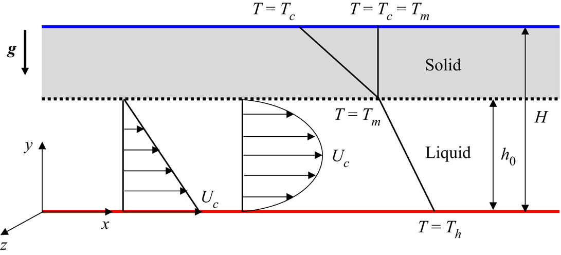
We consider a pure substance enclosed between two parallel plates of distance H. The solid is fixed and bounded below by the liquid where a Couette/Poiseuille flow develops, see figure 1. A Cartesian coordinate system is chosen to describe the problem with the y-axis pointing vertically upward, i.e. opposite to gravity, and the x–z plane coinciding with the lower plate. Initially, the liquid occupies the extended layer contained in the range 0 < y < h 0, the solid occupies the layer h 0 < y < H and the solid–liquid interface is planar and located at y = h 0. The upper and lower plates are maintained at temperatures Tc and Th, respectively, which satisfy Th > Tm ≥ Tc, where Tm is the melting temperature of the substance. Note that Tm > Tc corresponds to a conducting solid while Tm = Tc corresponds to an isothermal solid. This will lead to two different boundary conditions as shown later.
Schematic of the physical problem. Note that, in the case of Poiseuille flow, Uc is the centreline velocity of the laminar flow.

We use subscripts l and s to denote variables in the liquid and solid, respectively. For simplicity, we assume that the liquid and solid have the same thermodynamical and transport properties, i.e. density, specific heat and thermal conductivity (Toppaladoddi & Wettlaufer Reference Toppaladoddi and Wettlaufer2019; Purseed et al. Reference Purseed, Favier and Duchemin2020; Couston et al. Reference Couston, Hester, Favier, Taylor, Holland and Jenkins2021). The coupled effects of shear flow, buoyancy-driven flow and phase change are described by the Boussinesq equations in the liquid, the heat diffusion equation in the solid and the Stefan condition at the interface (Davis et al. Reference Davis, Müller and Dietsche1984; Kim et al. Reference Kim, Lee and Choi2008; Toppaladoddi & Wettlaufer Reference Toppaladoddi and Wettlaufer2019). In the liquid, the governing equations under consideration are
 \begin{gather}\boldsymbol{\nabla }\boldsymbol{\cdot }\boldsymbol{U} = 0,\end{gather}
 \begin{gather}{\rho _0}\frac{{\partial \boldsymbol{U}}}{{\partial t}} + {\rho _0}(\boldsymbol{U}\boldsymbol{\cdot }\boldsymbol{\nabla })\boldsymbol{U} ={-} \boldsymbol{\nabla }P + \mu {\nabla ^2}\boldsymbol{U} + \rho \boldsymbol{g}\beta ({T_l} - {T_m}),\end{gather}
 \begin{gather}\frac{{\partial {T_l}}}{{\partial t}} + \boldsymbol{U}\boldsymbol{\cdot }\boldsymbol{\nabla }{T_l} = \alpha {\nabla ^2}{T_l},\end{gather}
where U = (U, V, W) is the velocity, ρ(ρ 0) the (reference) density, P the pressure, μ the kinetic viscosity, g the acceleration due to gravity, β the thermal expansion coefficient, Tl the temperature of the liquid and α the thermal diffusivity.
The heat diffusion equation in the solid is given by
 \begin{equation}\frac{{\partial {T_s}}}{{\partial t}} = \alpha {\nabla ^2}{T_s},\end{equation}
where Ts is the temperature of the solid.
At the interface, we have the Stefan condition (Davis et al. Reference Davis, Müller and Dietsche1984; Worster Reference Worster2000)
 \begin{equation}{T_l} = {T_s} = {T_m},\quad {\rho _0}L\frac{{\partial h}}{{\partial t}} = \boldsymbol{n} \cdot \lambda (\boldsymbol{\nabla }{T_s} - \boldsymbol{\nabla }{T_l}),\end{equation}
where L is the latent heat of fusion/melting, h = h(x, y, t) is the height of the interface, n is the unit normal vector to the interface and λ is the thermal conductivity. Note that, by replacing (2.5a) with Tl = Ts = Tm + Kiγ/L, where Ki and γ are twice the mean curvature of the interface and the interfacial energy, respectively, the Gibbs–Thompson effect can be included (Davis et al. Reference Davis, Müller and Dietsche1984). However, it is negligible in our problem with convective length scales (Vasil & Proctor Reference Vasil and Proctor2011).
The heated and cooled boundaries are considered perfectly conducting, i.e.
 \begin{equation}{T_l} = {T_h},\;\textrm{at}\;y = 0\quad \textrm{and}\quad {T_s} = {T_c},\;\textrm{at}\;y = H.\end{equation}
The boundary conditions for the velocity field are twofold. For the case with Poiseuille flow and the case without external flow, the lower and upper boundaries of the liquid are considered no-slip, i.e.
 \begin{equation}\boldsymbol{U} = \textbf{0}\;\textrm{at}\;y = 0\quad \textrm{and}\quad y = {h_0}.\end{equation}
For the case of Couette flow, we have
 \begin{equation}U = {U_c},\quad V = W = 0\;\textrm{at}\;y = 0\quad \textrm{and}\quad U = V = W = 0\;\textrm{at}\;y = {h_0}.\end{equation}
Following Toppaladoddi & Wettlaufer (Reference Toppaladoddi and Wettlaufer2019), we introduce the following scales:
 \begin{equation}x,y,z \sim {h_0},\quad t \sim h_0^2/\alpha ,\quad U,V,W \sim {U_c},\quad p \sim {\rho _0}{U_c}\alpha /{h_0},\quad {T_l},{T_s} \sim {T_h} - {T_m}.\end{equation}
Applying these scales to non-dimensionalize (2.1)–(2.5) and using the same symbols as before to denote non-dimensional variables, we have the following dimensionless equations:
 \begin{gather}\boldsymbol{\nabla }\boldsymbol{\cdot }\boldsymbol{U} = 0,\end{gather}
 \begin{gather}\frac{{\partial \boldsymbol{U}}}{{\partial t}} + Pe(\boldsymbol{U}\boldsymbol{\cdot }\boldsymbol{\nabla })\boldsymbol{U} ={-} \boldsymbol{\nabla }p + Pr{\nabla ^2}\boldsymbol{U} + \frac{{RaPr}}{{Pe}}{T_l}\boldsymbol{y},\end{gather}
 \begin{gather}\frac{{\partial {T_l}}}{{\partial t}} + Pe\boldsymbol{U}\boldsymbol{\cdot }\boldsymbol{\nabla }{T_l} = {\nabla ^2}{T_l},\end{gather}
 \begin{gather}\frac{{\partial {T_s}}}{{\partial t}} = {\nabla ^2}{T_s},\end{gather}
 \begin{gather}St\frac{{\partial h}}{{\partial t}} = \boldsymbol{n}\boldsymbol{\cdot }(\boldsymbol{\nabla }{T_s} - \boldsymbol{\nabla }{T_l}).\end{gather}
The dimensionless parameters appearing in the above equations are the Péclet number Pe, which measures the relative importance of advection versus thermal diffusion here, the Prandtl number Pr, which compares the kinematic viscosity with thermal diffusivity, the Rayleigh number Ra, which represents the ratio of the buoyancy to the viscous force, and the Stefan number St, which controls the rate of melting/freezing. They are given by
 \begin{equation}Pe = \frac{{{U_c}{h_0}}}{\alpha },\quad Pr = \frac{\nu }{{{\alpha _l}}},\quad Ra = \frac{{g\beta ({T_h} - {T_m})h_0^3}}{{\nu \alpha }},\quad St = \frac{L}{{{c_p}({T_h} - {T_m})}}.\end{equation}
Note that, for convenience, the Prandtl number is fixed to be unity throughout the paper, unless otherwise mentioned (later we will show the Prandtl number independence for Pr > 1). In this situation, we have Pe = Re, where Re = Uch 0/ν is the Reynolds number; this means that Pe can be seen as the measure of the intensity of the shear flow.
Now, the thermal boundary conditions become
 \begin{equation}{T_l} = 1\;\textrm{at}\;y = 0;\quad {T_l} = {T_s}\;\textrm{at}\;y = 1;\quad {T_s} = 0\;\textrm{at}\;y = H.\end{equation}
For Couette flow, the velocity boundary conditions become
 \begin{equation}U = 1,\quad V = W = 0\;\textrm{at}\;y = 0;\;U = V = W = 0,\;\textrm{at}\;y = 1,\end{equation}
whereas for no external flow or Poiseuille flow, we have
 \begin{equation}U = V = W = 0\;\textrm{at}\;y = 0\quad \textrm{and}\quad y = 1.\end{equation}
One should note that, for a thermal boundary condition, if Tl(y = 1) = Ts(y = 1) = Ts(y = H) = 0, the liquid layer will slowly deepen until all of the solid melts so that the system will be time dependent, whereas if Tl(y = 1) = Ts(y = 1) > Ts(y = H) = 0, the system can reach a steady state before all the solid melts. This will be further discussed in detail in § 3.
3. Linear stability analysis
The linear stability theory that we will adopt here deals with the evolution of a disturbance of small amplitude superposed on a laminar/hydrostatic base flow (Schmid & Henningson Reference Schmid and Henningson2001). Generally, the evolution equations for the disturbance can be derived by decomposing the flow variable as a sum of base state and perturbation. In this section, we first introduce various types of the base state of temperature and velocity fields, then we derive the perturbation equations governing the development of a disturbance on the given base state.
3.1. Base state
In the base state, the interface is planar and located at y = 1. Depending on the melting temperature Tm, two kinds of base state exist: for Th > Tm > Tc, the system possesses a steady base state (SBS) (Davis et al. Reference Davis, Müller and Dietsche1984; Toppaladoddi & Wettlaufer Reference Toppaladoddi and Wettlaufer2019), whereas for Th > Tm = Tc, the system possesses a quasi-steady base state (QBS) in the large-Stefan-number limit (Kim et al. Reference Kim, Lee and Choi2008; Vasil & Proctor Reference Vasil and Proctor2011).
In SBS, the initial thicknesses of the liquid and solid layers are constant, depending on  $\varLambda$, the ratio of the temperature differences across the liquid and the solid regions, i.e. (Davis et al. Reference Davis, Müller and Dietsche1984)
 \begin{equation}\varLambda = \frac{{{T_m} - {T_c}}}{{{T_h} - {T_m}}}.\end{equation}
In the SBS, the temperatures in the liquid and solid are purely conductive, i.e.
 \begin{equation}\overline {{T_l}} = 1 - y,\quad \overline {{T_s}} = \frac{\varLambda }{{H - 1}}(1 - y).\end{equation}
Assuming that the heat fluxes away from and towards the interface balance, the Stefan condition becomes
 \begin{equation}\frac{{\textrm{d}\overline {{T_l}} }}{{\textrm{d}y}} - \frac{{\textrm{d}\overline {{T_s}} }}{{\textrm{d}y}} = 0,\quad \textrm{at}\;y = 1,\end{equation}
which gives
 \begin{equation}\varLambda = H - 1.\end{equation}
This means that, in steady state, the dimensionless thickness of the solid equals to the ratio of temperature difference (Davis et al. Reference Davis, Müller and Dietsche1984; Toppaladoddi & Wettlaufer Reference Toppaladoddi and Wettlaufer2019). Note that H in (2.20) is dimensionless.
In QBS, the system has an inherently time-dependent background state of the temperature field. Since the solid does not conduct heat, we have the simplified balances as follows (Vasil & Proctor Reference Vasil and Proctor2011):
 \begin{equation}\frac{{\partial {T_l}}}{{\partial t}} = \frac{{{\textrm{d}^2}{T_l}}}{{\textrm{d}{\textrm{y}^2}}},\quad {\left. {St\frac{{\partial h}}{{\partial t}} ={-} \frac{{\textrm{d}{T_l}}}{{\textrm{d}y}}} \right|_{y = \eta }},\end{equation}
which admits the following solutions:
 \begin{equation}{T_l}(t,y) = 1 - \frac{{\textrm{erf}(\kappa y/h(t))}}{{\textrm{erf}(\kappa )}},\quad h(t) = 2\kappa \sqrt t ,\end{equation}
where erf is the error function, given by
 \begin{equation}\textrm{erf}(\xi ) = \frac{2}{{\sqrt{ {\rm \pi}} }}\int_0^\xi {{\textrm{e}^{ - \xi _0^2}}\,\textrm{d}{\xi _0}} ,\end{equation}
and κ is the root of the following transcendental equation
 \begin{equation}St = \sqrt{ {\rm \pi}} \kappa \textrm{erf}(\kappa )\exp ({\kappa ^2}).\end{equation}
It is clear that the base state (2.22) is time dependent. However, in the large-Stefan-number limit, the melting of the interface will be very slow so that the system can possess a QBS, in which the thickness of the liquid is constant and the temperature distribution asymptotes to (2.18a). For details, please refer to Appendix A.
For the base state of the velocity field, we consider three different cases. The first one is the hydrostatic state, which means that no shear flow is imposed, i.e.
 \begin{equation}\bar{\boldsymbol{U}} = \textbf{0}.\end{equation}
In the second case we introduce a steady Couette flow, in which
 \begin{equation}\bar{U} = 1 - y,\quad V = W = 0.\end{equation}
In the third case a steady Poiseuille flow is imposed, in which
 \begin{equation}\bar{U} = 4y(1 - y),\quad V = W = 0.\end{equation}
One should note that the flow of ambient fluid is much more complex in the natural setting (Hewitt Reference Hewitt2020). We nevertheless consider both Couette and Poiseuille flows here to investigate the effect of external flow (Toppaladoddi & Wettlaufer Reference Toppaladoddi and Wettlaufer2019; Couston et al. Reference Couston, Hester, Favier, Taylor, Holland and Jenkins2021; Toppaladoddi Reference Toppaladoddi2021).
3.2. Equations for the perturbation
Following Davis et al. (Reference Davis, Müller and Dietsche1984) and Kim et al. (Reference Kim, Lee and Choi2008), we introduce the following normal mode to separate variables into base state and perturbation:
 \begin{gather}F(x,y,z,t) = \bar{F}(y) + f(y)\exp ( - \textrm{i}\omega t)\exp (\textrm{i}kx + \textrm{i}mz) + \textrm{c}.\textrm{c}.,\end{gather}
where F represents any variable in (U, V, W, Tl, Ts)T,  $\bar{F}$ denotes the base state of F,f = (u, v, w, θl, θs) is the shape function, k and m are real-valued streamwise and spanwise wavenumbers, ω is the circular frequency of the perturbation and c.c. is the complex conjugate. Note that ω is complex valued with its real part being the phase speed and its imaginary part being the growth rate. Upon substitution of the above expression into the dimensionless equations (2.9)–(2.11), we arrive at a simplified set of equations in the liquid, i.e.
 \begin{gather}\textrm{i}ku + Dv + \textrm{i}mz = 0,\end{gather}
 \begin{gather}- \textrm{i}\omega u ={-} Pe(\textrm{i}k\bar{U}u + vD\bar{U}) - \textrm{i}kp + Pr({D^2} - {\gamma ^2})u,\end{gather}
 \begin{gather}- \textrm{i}\omega v ={-} \textrm{i}kPe\bar{U}v - Dp + \frac{{Ra \cdot Pr}}{{Pe}}{\theta _l} + Pr({D^2} - {\gamma ^2})v,\end{gather}
 \begin{gather}- \textrm{i}\omega w ={-} \textrm{i}kPe\bar{U}w - \textrm{i}mp + Pr({D^2} - {\gamma ^2})w,\end{gather}
 \begin{gather}- \textrm{i}\omega {\theta _l} ={-} Pe(\textrm{i}k\bar{U}{\theta _l} + vD\overline {{\theta _l}} ) + ({D^2} - {\gamma ^2}){\theta _l},\end{gather}
where D = d/dy and γ 2 = k 2 + m 2.
The boundary conditions for the perturbation are given as
 \begin{gather}u = v = w = 0,\;\textrm{at}\;y = 0,\textrm{ }1;\quad {\theta _l} = 0\;\textrm{at}\;y = 0\quad \textrm{for}\;\textrm{QBS}\;\textrm{and}\;\textrm{SBS,}\end{gather}
 \begin{gather}D{\theta _l} = 0\;\textrm{at}\;y = 1\quad \textrm{for}\;\textrm{QBS};\end{gather}
 \begin{gather}D{\theta _l} + {\theta _l}\gamma \coth (\gamma \varLambda ) = 0\;\textrm{at}\;y = 1\quad \textrm{for}\;\textrm{SBS}.\end{gather}
The perturbed temperature boundary conditions at the interface (2.34c,d) are derived from the Stefan condition (2.13). Specifically, the condition (2.34c) was originally given by Kim et al. (Reference Kim, Lee and Choi2008) and Vasil & Proctor (Reference Vasil and Proctor2011), which means that the interface acts as a fixed-flux boundary for QBS in the large-Stefan-number limit. The condition (2.34d) was derived by Davis et al. (Reference Davis, Müller and Dietsche1984) and coincides with the condition in Nield (Reference Nield1968), which indicates that the interface for SBS behaves like a planar rigid solid that is an imperfect thermal conductor.
For SBS, the equation for the perturbed temperature in the solid is given by
 \begin{equation}({D^2} - {\gamma ^2}){\theta _s} = 0,\end{equation}
with boundary conditions
 \begin{equation}{\theta _s} = {\theta _l}\;\textrm{at}\;y = 1\quad \textrm{and}\quad {\theta _s} = 0\;\textrm{at}\;y = 1 + \varLambda .\end{equation}
The perturbed temperature determined by (2.35) and (2.36) in the solid can be solved analytically, see Davis et al. (Reference Davis, Müller and Dietsche1984). The eigenvalue problem (in the liquid), (2.29)–(2.33), along with boundary conditions (2.34), is discretized with a spectral method (Weideman & Reddy Reference Weideman and Reddy2000). For clarity, we postpone the details of the numerical method and validation to Appendix B. Note that, in the following analysis, we mainly focus on the dynamics of the melt layer.
4. Results of stability analysis
For convenience, we will hereafter use RBC_M (respectively RBC) and RBP_M (respectively RBP) to represent the RB–Couette flow and the RB–Poiseuille flow in the presence (respectively absence) of a phase boundary. We first analyse the combined effects of the phase boundary and shear on buoyancy-driven instability for QBS, then the case of SBS will be discussed. Note that we consider a two-dimensional problem with spanwise wavenumber m = 0, which means that we consider the instability of transverse rolls. The reason for such a choice is given in Appendix C.
4.1. Linear stability for QBS
We show in figure 2 the perturbed velocity and the perturbed temperature field in the liquid for RB convection with four different configurations. Compared with figure 2(a) for classical cases, in the presence of a melting boundary a non-trivial change of the distribution of the isotherm near y = 1 (representing the interface) is observed, as shown in figure 2(c). This is due to the fact that, compared with RB, the specificity of melting-boundary convection (RB_M) lies in the temperature boundary conditions at the interface between the solid and liquid phases. For RB, both the cold top boundary and the heated bottom boundary are considered perfectly conducting, whereas in the case of melting-boundary convection, the dynamics proceeds with a fixed-flux condition, i.e. Dθl = 0 at y = 1 near the onset of flow motion (Kim et al. Reference Kim, Lee and Choi2008; Vasil & Proctor Reference Vasil and Proctor2011). On the other hand, since the no-slip boundary condition is still valid as before in the large-Stefan-number limit, we do not observe any obvious difference in the perturbed velocity fields between the classical and present cases, as shown in figures 2(b) and 2(d).
Perturbed temperature fields in the liquid (a,c,e,g) and perturbed velocity fields (b,d,f,h) for classical RB ((a) and (b)), RB_M ((c) and (d)), RBC_M ((e) and (f)) and RBP_M ((g) and (h)). The parameters are Ra = 2000 for (a–h), and Pe = 10 for (e–h). The wavelength λ occurring in the x-ordinate is such that λ = 2 ${\rm \pi}$/k, where k is 2.748.

Once the effect of shear is considered, the system is expected to exhibit a more complex dynamics. To iterate, we consider the instability of transverse rolls whose axes are perpendicular to the direction of mean shear. In this situation, perturbations in the liquid are influenced as soon as the shear is imposed (Chung & Chen Reference Chung and Chen2001; Neufeld & Wettlaufer Reference Neufeld and Wettlaufer2008; Toppaladoddi & Wettlaufer Reference Toppaladoddi and Wettlaufer2019). Our calculations are consistent with this understanding. As shown in figure 2(e–h), we observe the distortions of the perturbed temperature and velocity fields under the effects of shear. It appears that, in RBP_M, the convective rolls are less distorted compared with RBC_M, which is due to the symmetry of Poiseuille flow with respect to the centreline.
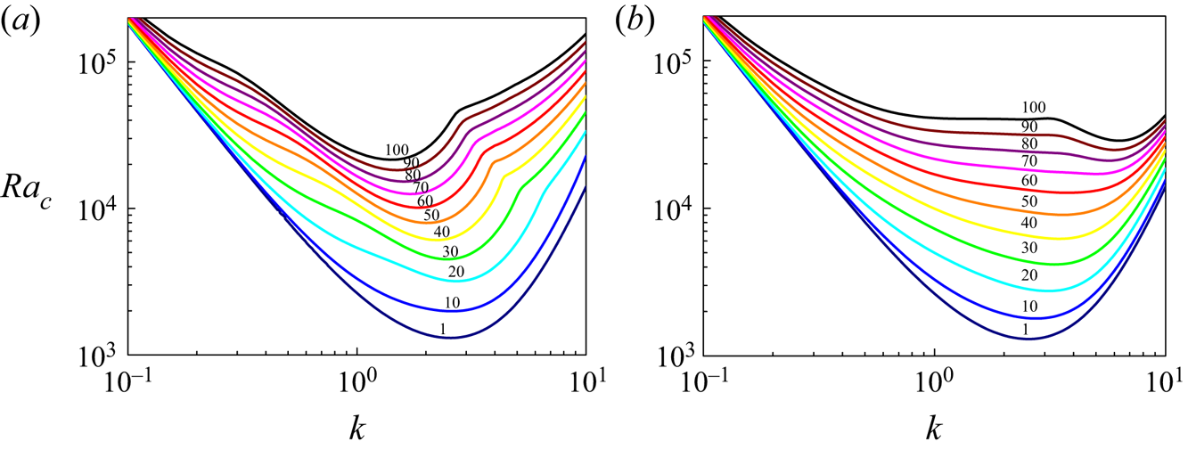
Figure 3 presents the neutral stability curves for different Pe. It is seen that the imposed shear flow leads to the stabilization of the convection, which is evidenced by the increase of Rac with larger values of Pe. This result bears remarkable resemblance to Gallagher & Mercer (Reference Gallagher and Mercer1965) and Gage & Reid (Reference Gage and Reid1968) in which the authors found that the instability of transverse rolls tends to be suppressed by Couette/Poiseuille flow in classical stratified shear flows. The critical Rayleigh number and wavenumber are plotted as functions of Pe in figure 4. The solutions for RBC, RBP with perfectly conducting boundary are also shown for comparison purposes. Regarding the reasons responsible for the increase of Rac with increasing Pe, we resort to an energy analysis in § 5. Here, it is found that there are three instability modes in the present system. The first mode is dominated by the boundary condition, so it is named the boundary mode, which dominates for Pe < 10. As shown in figure 4(a), in the absence of a melting boundary, Rac is close to 1707.763 (Chandrasekhar Reference Chandrasekhar1961), the stability threshold of classical RB; whereas in the presence of a melting boundary, Rac is expected to approach 1295.778, the stability threshold of RB_M for QBS (Vasil & Proctor Reference Vasil and Proctor2011). The bulk flow mode is dominant for Pe > 40, see figure 4(c), in which the system is governed by the bulk flow and the variation of Rac depends on the kind of shear imposed, independent of condition at the upper boundary. The final mode, namely the mixed boundary–bulk mode, lies between the aforementioned two modes. As shown in figure 4(b), the mixed mode is affected simultaneously by the boundary conditions and base flows.
The marginal stability curves plotted in the Ra–k plane, with the values of Pe marked on the lines. (a): RB–Couette flow with melting boundary; (b): RB–Poiseuille flow with melting boundary.

Critical Rayleigh number (a–c) and critical wavenumber (d) as functions of Péclet number. Panels (a), (b) and (c) correspond to the boundary mode, mixed mode and bulk flow mode, respectively.

The variation of kc is consistent with that of Rac, see figure 4(d). In the boundary mode, the value of kc depends on the boundary condition imposed. For the perfectly conducting condition, kc approaches 3.116 (Chandrasekhar Reference Chandrasekhar1961), whereas for the melting-boundary condition, kc approaches 2.552 (Vasil & Proctor Reference Vasil and Proctor2011). In the bulk flow mode, when the Couette flow is imposed, kc tends to decrease with increasing Pe, whereas in Poiseuille cases kc tends to increase with larger values of Pe. Between these two modes, we observe that different curves intersect. The decrease of kc with Pe in Couette cases is consistent with the result in Gallagher & Mercer (Reference Gallagher and Mercer1965), whereas the increase of kc with Pe in Poiseuille cases appears to be unconventional since the Poiseuille flow will be unstable at Re = 5772.2 and k = 1.02. In fact, this observation is not contradictory itself. It is noted that two instabilities exist in the stratified Poiseuille flow: buoyancy-driven instability, and the Tollmien–Schlichting instability (Gage & Reid Reference Gage and Reid1968). When the shear is weak, convective instability dominates, with the critical wavenumber increasing with shear intensity. For sufficiently strong shear intensity, however, the Tollmien–Schlichting instability plays the main role, with the corresponding critical wavenumber being k = 2.04 (note that our length scale is the height of the liquid).
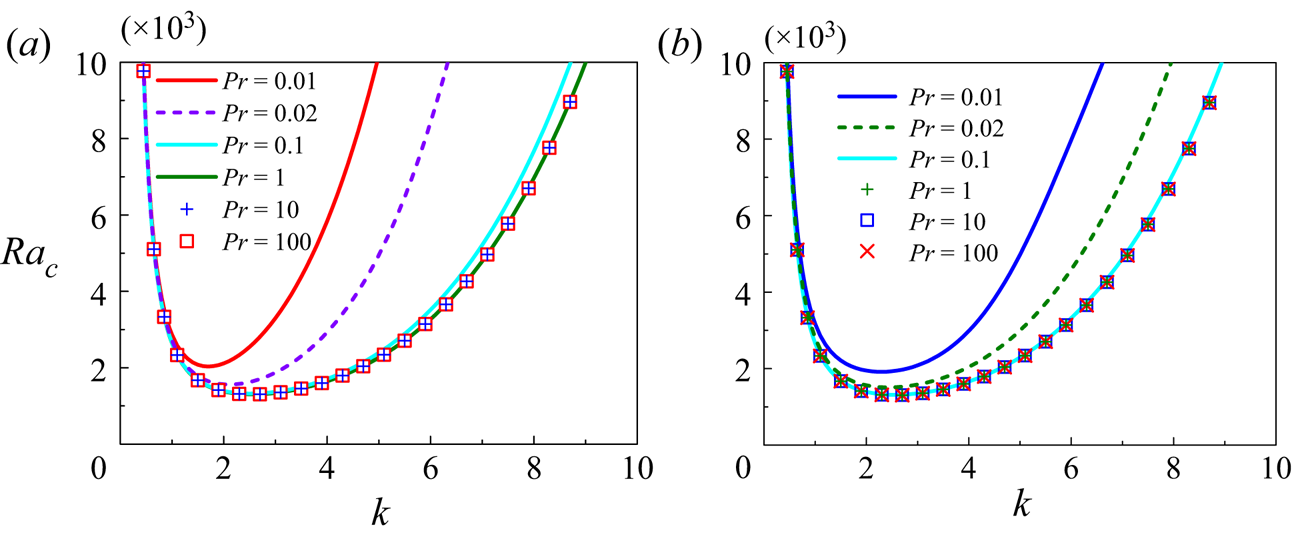
It is interesting to consider the influence of the Prandtl number Pr. In order to isolate the effect of Pr, here, the Reynolds number, i.e. Re = Pe/Pr, is fixed at Re = 1. Note that in classical RB (Chandrasekhar Reference Chandrasekhar1961) and RB_M in the large-Stefan-number limit (Davis et al. Reference Davis, Müller and Dietsche1984; Vasil & Proctor Reference Vasil and Proctor2011), the linear stabilities of the systems are independent of Pr, except that in the case of RB with a fast melting boundary Rac and kc tend to decrease with Pr (Kim et al. Reference Kim, Lee and Choi2008). Considering the combined effects of slowly melting boundary and shear flow, as shown in figure 5, the convective instability tends to be suppressed as Pr increases. In the limit of small Prandtl number, Pr has a greater influence on the stability of the system compared with the large-Prandtl-number limit in which Rac tends to asymptote. The Pr dependence shown here might be due to the interaction between the temperature gradient and shear flow instead of melting boundary, since Rac and γc are functions of Pe and Pr for thermally stratified shear flow without a melting boundary (Fujimura & Kelly Reference Fujimura and Kelly1988).
Effect of Pr: neutral stability curves in the presence of (a) Couette flow and (b) Poiseuille flow. Here, the Reynolds number, i.e. Re = Pe/Pr, is fixed at Re = 1.

4.2. Linear instability of SBS
We now turn to a melting/freezing system in which the solid can conduct heat away from the interface so that a SBS is assumed. This system has been originally studied by Davis et al. (Reference Davis, Müller and Dietsche1984) and extended by Toppaladoddi & Wettlaufer (Reference Toppaladoddi and Wettlaufer2019) to consider the effect of low-Pe Couette flow. Here, the Poiseuille flow is newly considered, and a more systematic investigation of the convective instability under the combined effects of shear and a phase boundary is performed. Compared with QBS where there is no heat conduction in the solid, the principal characteristic of SBS is that the thickness of the solid denoted by  $\varLambda$ affects the instability of the system.
We first consider the case in the absence of shear in which the stability is governed by the parameter  $\varLambda$. In figure 6(a–c) the perturbed temperature fields in the liquid and the solid are shown. The horizontal red lines represent the interface. When the solid layer is very thin, as shown in figure 6(a), the effect of the interface is so weak that the perturbed temperature is identical to that for classical RB; see figure 2(a). As
 $\varLambda$ increases, the effects of the solid–liquid interface become intense so that one observes in figure 6(b) a perturbed temperature field similar to the case with a fixed-flux condition shown in figure 2(c). Further increasing
 $\varLambda$, the heat flux across the interface becomes more intense, see figure 6(c). In panel (d), we show the amplitude of the perturbed temperature in the liquid and the solid for x = 0 and x = λ/2. A continuous profile of amplitude at the solid–liquid interface is readily seen, which is consistent with Kim et al. (Reference Kim, Lee and Choi2008).
Perturbed temperature in the liquid and solid. The parameters are such that  $\varLambda$ = 0.001, Ra = 1710, k = 3.116 for (a),
 $\varLambda$ = 0.1, Ra = 1620, k = 3.028 for (b) and
 $\varLambda$ = 1, Ra = 1510, k = 2.819 for (c) and (d). The shear flow is not considered here, i.e. Pe = 0. The horizontal red dashed lines in (a–c) represent the solid–liquid interface. Panel (d) corresponds to the amplitude of the perturbed temperature at x = 0 and x = λ/2 (denoted by the vertical dash-dotted lines in (a–c)).

The critical Rayleigh number and wavenumber as functions of  $\varLambda$ have been given by Davis et al. (Reference Davis, Müller and Dietsche1984) and Toppaladoddi & Wettlaufer (Reference Toppaladoddi and Wettlaufer2019); see figure 16 in Appendix B. It is seen that Rac and kc decrease with increasing
 $\varLambda$. This is due to the fact that, at the onset of convection, the planar interface behaves like an imperfect thermal conductor. With the increase of
 $\varLambda$, the interface becomes a worse conductor and therefore Rac decreases, whereas as
 $\varLambda$ gets close to 0, the interface becomes a perfect thermal conductor so that (2.29)–(2.33) are reduced to the classical RB equations (Davis et al. Reference Davis, Müller and Dietsche1984).
Now we consider the case in the presence of shear flow. We show in figures 7 and 8 the perturbed temperature and velocity for various Pe in the presence of Couette and Poiseuille flows, respectively. It is obvious that the isotherms and the convective rolls are distorted once the shear flow is imposed, consistent with the results for QBS. In particular, in the case of RBC_M, even though the distortion effect is more intense when the intensity of the shear flow increases, near the interface (see y > 0.8 in figure 7c) the isotherm is still affected by the phase boundary. This is different from the case of RBP_M in which the perturbed temperature becomes independent of the phase boundary for Pe = 100. The isotherms exhibit a structural symmetry with respect to y = 0.5, as shown in figure 8(c).
Perturbed temperature fields in the liquid ((a) and (c)) and velocity fields ((b) and (d)) for  $\varLambda$ = 0.2 in the presence of Couette flow. The parameters are Pe = 10, Ra = 1980, k = 2.808 for (a) and (b), and Pe = 100, Ra = 21 840, k = 1.416 for (c) and (d).

Perturbed temperature fields in the liquid ((a) and (c)) and velocity fields ((b) and (d)) for  $\varLambda$ = 1 in the presence of Poiseuille flow. The parameters are Pe = 10, Ra = 1830, k = 2.891 for (a) and (b), and Pe = 100, Ra = 28 710, k = 6.297 for (c) and (d).

Regarding the combined effects of solid depth and shear intensity on convective instability, we present a series of plots in figure 9 to characterize the features. Figure 9(a) shows the critical Rayleigh number Rac for a wide range of Pe and  $\varLambda$ when Couette flow is considered. It is seen that, with the influence of solid depth appearing to be insignificant relative to the shear flow, the system is unstable to vertical convection at higher Rac for larger values of shear velocity. To highlight the interplay between the shear and phase boundary, we normalize Rac in a way such that
 $R{a_{cn}} = (R{a_c} - R{a_{cmin}})/ (R{a_{cmax}} - R{a_{cmin}})$, where
 $R{a_{c\,max}} = max\{ R{a_c}|0 \le \varLambda \le 1\}$ and
 $R{a_{cmin}} = min\{ R{a_c}|0 \le \varLambda \le 1\}$ for a given Pe. The results are presented in figure 9(b). It is clear that, with the increase of shear intensity, the threshold of convection first transitions from a decreasing function of the solid depth to an increasing one, but finally returns to a decreasing function for sufficiently strong shear intensity. Moreover, during the transition, i.e. 11 < Pe < 14 and 70 < Pe < 80, the convective instability has little dependence on phase boundary, as evidenced by figure 9(d) in which we show
 $\Delta R{a_c} = R{a_{cmax}} - R{a_{cmin}}$ as a function of Pe. Away from the two regimes, the Couette flow surprisingly enhances the phase boundary dependence of the convective instability. This behaviour indicates that the effects of interface should not be overlooked in the present system. Furthermore, it is drawn from the above observations that the instability of the present system is dominated by a mixed mode, in which the effect of the interface is weaker than the shear (see figure 9a), but not negligible. Here, we also show the variation of the critical wavenumber kc as a function of the solid thickness. As shown in figure 9(c), similar to the case of QBS, here, when Couette flow is imposed, kc is expected to decrease for larger values of Pe, while at the same time, it evolves from a decreasing function of the solid depth to an increasing function with the increase of the shear intensity.
The dependence of the instability on the shear and phase boundary with (a–c) corresponding to RBC_M and (e–h) corresponding to RBP_M. Specifically, (a) and (e) show Rac as a function of Pe and  $\varLambda$; (b) and (f) show normalized Rac, i.e.
 $R{a_{cn}} = (R{a_c} - R{a_{cmin}})/(R{a_{cmax}} - R{a_{cmin}})$, where
 $R{a_{cmax}} = max\{ R{a_c}|0 \le \varLambda \le 1\} ,R{a_{cmin}} = min\{ R{a_c}|0 \le \varLambda \le 1\}$ for a given Pe; (c), (g) and (h) show kc as a function of
 $\varLambda$ with Pe increasing from 0 to 100; (d) shows
 $\Delta R{a_c} = R{a_{cmax}} - R{a_{cmin}}$ as a function of Pe.

The case of imposed Poiseuille flow has some similarities with the former case, e.g. the shear has a more intense effect on the convection threshold than the phase boundary, see figure 9(e). However, it also has some distinguishing features in its own right. As shown in figure 9(f), the convective instability shows a different phase boundary dependence when the intensity of Poiseuille flow is sufficiently strong. In particular, for Pe > 80, the thickness of the solid layer has negligible influence on Rac, which can be further evidenced by figure 9(d). This indicates that the Poiseuille flow, when it increases in intensity, tends to eliminate the effect of the phase boundary. Therefore, below a critical Péclet number, which is Pe = 80 in our calculation, the system is dominated by the mixed mode. Above the critical value, however, the effect of the interface becomes negligible so that the bulk flow mode dominates the instability. In § 5 we will discuss the mechanism accounting for the different characteristics between the Couette and the Poiseuille flow cases. In contrast to the case of imposed Couette flow, here, the critical wavenumber is an increasing function of Pe, which, as shown in figures 9(g) and 9(h), has a very slow growth rate for Pe < 60; after that, however, a rapid growth is readily seen until Pe = 70.
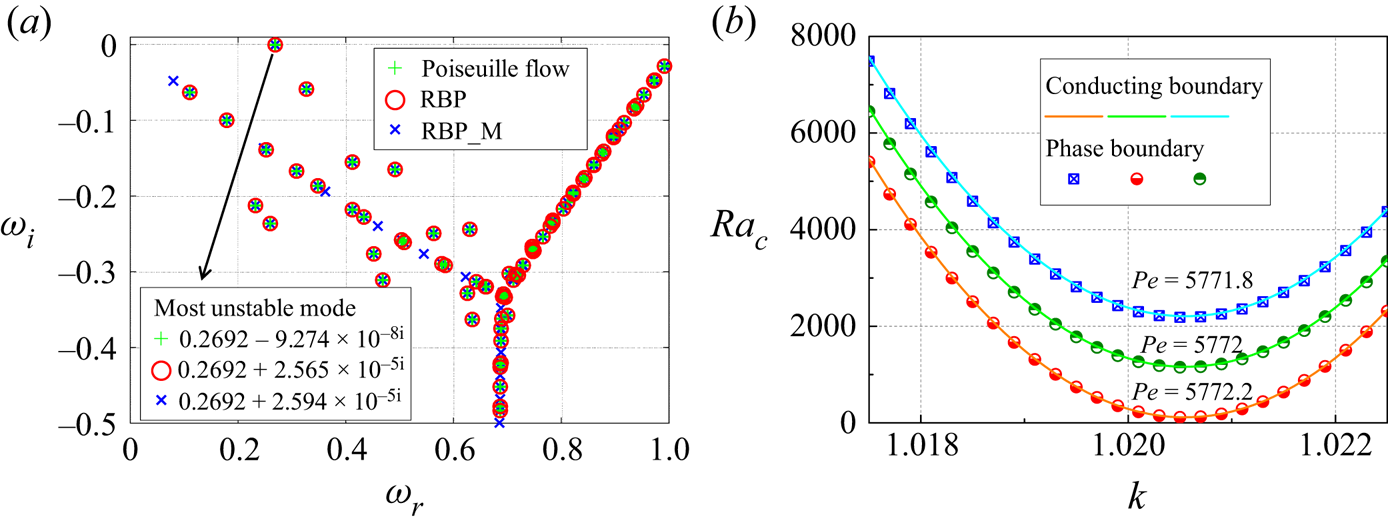
Finally, it is interesting to consider the dynamics with high-Pe Poiseuille flow. In this situation the Tollmien–Schlichting instability will be important. We focus on the system of SBS with a large  $\varLambda$ to ensure that the effect of interface is sufficiently strong. As shown in figure 10(a), in the case of high-Pe Poiseuille flow, the core modes, wall modes and centre modes do not change appreciably under the effects of the temperature gradient and solid–liquid interface. The imaginary part of the most unstable mode, however, changes sign, indicating that the system becomes unstable in the presence of a temperature gradient and/or interface; see figure 10(a). This also indicates that the buoyancy is still a destabilizing factor in this situation. The effect of high-Pe Poiseuille flow on the stability of the solid–liquid phase-change system is shown in figure 10(b). It is obvious that the boundary condition has a negligible effect on the marginal stability in comparison with shear, indicating that the instability is dominated by the bulk flow mode in the high-Pe regime. In addition, we observe that convective instability occurs at a lower Rayleigh number with higher Pe for all wavenumbers. This observation is profoundly dissimilar to the low-Pe cases, which is due to the fact that, in high-Pe Poiseuille flow, the dynamic instability from the base flow is dominant in destabilizing the system.
(a) Comparison of three spectra for Poiseuille flow, RBP and RBP_M. The parameters are Pe = 5772.2, k = 1.02 for all cases, Ra = 104 for RBP and RBP_M, and  $\varLambda$ = 5 for RBP_M. (b) Effect of high-Pe Poiseuille flow on the neutral stability curve for
 $\varLambda$ = 5.

5. Results of energy analysis
In order to interpret the physical mechanisms behind the results of the modal stability analysis, an energy analysis is performed in this section. Before proceeding to the analysis, it is necessary to briefly introduce the theory of energy analysis used here. Multiplying the linearized equation for fluid flow by the complex conjugate of the perturbation velocity  $v_i^{\dagger}$, we obtain the governing equation for the kinetic energy, i.e.
 \begin{equation}v_i^{\dagger} \frac{{\partial {v_i}}}{{\partial t}} + v_i^{\dagger} {v_j}Pe\frac{{\partial {{\overline U }_i}}}{{\partial {x_j}}} + v_i^{\dagger} {\overline U _j}Pe\frac{{\partial {v_i}}}{{\partial {x_j}}} ={-} v_i^{\dagger} \frac{{\partial p}}{{\partial {x_i}}} + v_i^{\dagger} Pr\frac{{{\partial ^2}{v_i}}}{{\partial x_j^2}} + v_i^{\dagger} \frac{{Ra\,Pr}}{{Pe}}{\theta _l}.\end{equation}
Taking the complex conjugate of the above equation and averaging the two equations, we obtain
 \begin{equation}\begin{array}{ccccc} \dfrac{{\partial E}}{{\partial t}} & ={-} \dfrac{1}{2}Pe(v_i^{\dagger} {v_j} + v_j^{\dagger} {v_i})\dfrac{{\partial {{\overline U }_i}}}{{\partial {x_j}}} - Pr\dfrac{{\partial v_i^{\dagger} }}{{\partial {x_j}}}\dfrac{{\partial {v_i}}}{{\partial {x_j}}} + \dfrac{1}{2}\dfrac{{Ra\,Pr}}{{Pe}}({\theta _l}v_i^{\dagger} + \theta _l^{\dagger} {v_i}){x_i}\\ & \quad + \dfrac{\partial }{{\partial {x_j}}}\left[ { - \dfrac{1}{2}v_i^{\dagger} {v_i} - \dfrac{1}{2}(pv_i^{\dagger} + p_i^{\dagger} {v_i}) + \dfrac{1}{2}Pr\left( {v_i^{\dagger} \dfrac{{\partial {v_i}}}{{\partial {x_j}}} + {v_i}\dfrac{{\partial v_i^{\dagger} }}{{\partial {x_j}}}} \right)} \right], \end{array}\end{equation}
where  $E = v_i^{\dagger} {v_i}/2$ is the perturbation energy density. Note that the terms in the square brackets are transport terms which make no contribution to the energy balance when a periodic boundary condition is imposed. Therefore, integrating (5.2) over the control volume Ω leads to
 \begin{align} \int_\varOmega {\dfrac{{\partial E}}{{\partial t}}\,\textrm{d}V} & ={-} \dfrac{1}{2}Pe\int_\varOmega {(v_i^{\dagger} {v_j} + v_j^{\dagger} {v_i})\dfrac{{\partial {{\overline U }_i}}}{{\partial {x_j}}}\,\textrm{d}V\quad \textrm{Prod}} \nonumber\\ &\quad - Pr\int_\varOmega {\dfrac{{\partial v_i^{\dagger} }}{{\partial {x_j}}}\dfrac{{\partial {v_i}}}{{\partial {x_j}}}\,\textrm{d}V\quad \textrm{VD}} \nonumber\\ & \quad + \dfrac{1}{2}\dfrac{{Ra\,Pr}}{{Pe}}\int_\varOmega {({\theta _l}v_i^{\dagger} + \theta _l^{\dagger} {v_i}){x_i}\,\textrm{d}V\quad \textrm{VT}} . \end{align}
The first term on the right-hand side corresponds to energy production from the external shear flow (denoted by Prod), which is zero in the absence of base flow. The second term, denoted by VD, represents viscous dissipation. The last term is denoted by VT and represents the energy exchange between the perturbed velocity field and temperature field.
5.1. Energy analysis for QBS
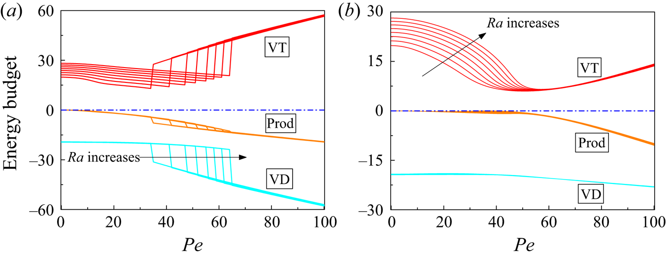
Regarding the combined effects of melting boundary and shear on the stability of RB convection, the energy budget for RBC_M and RBP_M in a wide range of Pe is shown in figure 11. Note that here Ra and k are fixed to isolate the effect of shear, and therefore one should expect a different Pe range of the mixed mode. We first note that the values of VT are positive, indicating that buoyancy is an important destabilizing factor of the system. In contrast, the values of VD are always negative, consistent with the idea that viscous dissipation damps the instability of flow. One of the mechanisms by which low-Pe Couette flow stabilizes the system in the boundary mode is achieved by inhibiting the upward heat flux, which is evidenced by the decrease of VT as Pe increases. We denote this mechanism by IHF (namely inhibiting heat flux). In Toppaladoddi & Wettlaufer (Reference Toppaladoddi and Wettlaufer2019), IHF is considered as the main mechanism by which Couette flow inhibits the instability of the phase boundary. Note that Toppaladoddi & Wettlaufer (Reference Toppaladoddi and Wettlaufer2019) mainly focused on the case of RBC_M with SBS for Pe < 5. Through the energy analysis, here we identify another mechanism which was not discussed by Toppaladoddi & Wettlaufer (Reference Toppaladoddi and Wettlaufer2019). As shown in figure 11(a), the values of Prod are negative in the presence of Couette flow, implying that Couette flow can also inhibit the growth of disturbance by absorbing energy from the perturbed hydrodynamic field. We denote the second mechanism by AE (namely absorbing energy) for convenience. As shown in figure 11(b), in RBP_M the effect of AE mechanism is negligible in boundary mode compared with the IHF mechanism.
Energy budget for (a) RBC_M and (b) RBP_M at k = 2.552. The Rayleigh number increases from 1500 to 5000 with intervals of 500. The horizontal dashed-dotted blue lines correspond to the zero value line.

For both RBC_M and RBP_M, in the mixed mode the effect of the IHF mechanism becomes unimportant while the effect of the AE mechanism becomes significant. More importantly, in the bulk flow mode, shear enhances the energy transfer from the thermal field to the hydrodynamic fluctuation. As a result, the AE mechanism becomes the primary factor by which shear stabilizes the system. It is necessary to explain why VT increases with Pe in the bulk flow mode. Similar to the externally imposed temperature boundary conditions in classical RB, it has been shown that viscous dissipation is also able to induce an unstable temperature gradient and thus thermal instability (Barletta & Nield Reference Barletta and Nield2010; Barletta, Celli & Nield Reference Barletta, Celli and Nield2011; Requilé et al. Reference Requilé, Hirata and Quarzazi2020a,Reference Requilé, Hirata, Quarzazi and Barlettab). The cause of this instability is the shear flow itself (Couette or Poiseuille flow) which acts as a heat source. Moreover, the onset of viscous instability is dependent on GePe 2, where Ge is the Gebhart number and is a constant here. Inspecting our results shown in figure 11, we note that, with the sharp growth of VT, the viscous dissipation curve, VD, goes through a clear decrease simultaneously. Besides, in the bulk flow mode, VT is an increasing function of Pe but independent of Ra. This is consistent with the idea of viscous dissipation induced thermal instability so that the increase of VT in bulk flow mode is believed to be attributed to this instability mechanism.
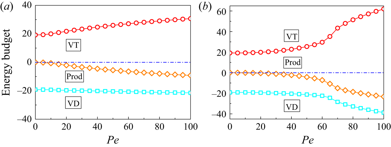
The energy budget analyses as functions of Pe while keeping Ra = Rac(Pe), k = kc(Pe) are also shown here; see figure 12. Since Rac is an increasing function of Pe, VT increases with shear intensity in the whole range of Pe as expected. On the other hand, since Prod and VD are only dependent on shear, their evolution trends with increasing Pe in figure 12 are similar to that in figure 11, despite that fact that no clear transition is observed in figure 12.
Energy budget for Rac and kc as functions of Pe: (a) RBC_M and (b) RBP_M.

5.2. Energy analysis for SBS
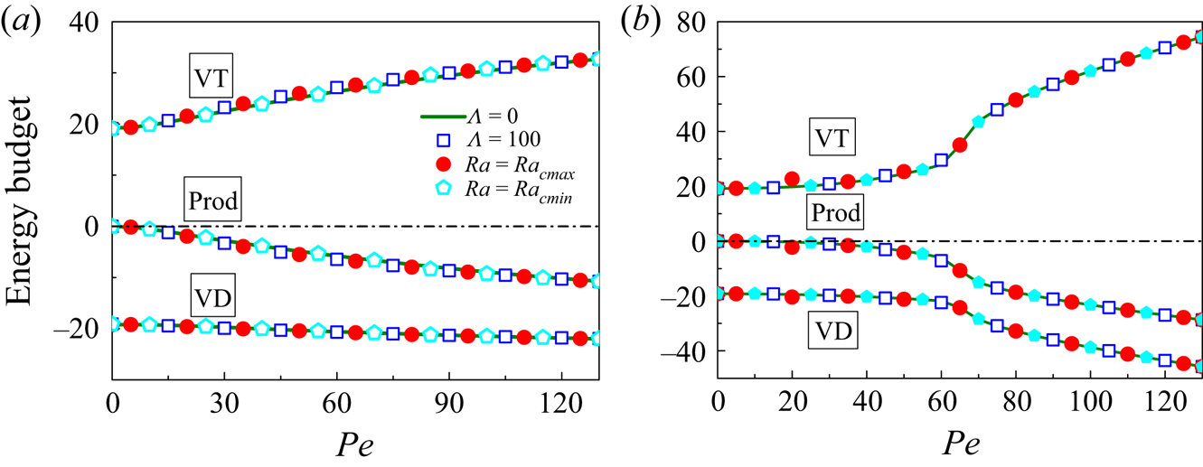
We now turn to the energy analysis for SBS. To provide a physical interpretation for the results in figures 9(d), we perform the energy analysis for RBC_M, RBP_M when keeping Ra = Rac( $\varLambda$, Pe), k = kc(
 $\varLambda$, Pe). As shown in figure 13, in order to highlight the effect of
 $\varLambda$, four cases of
 $\varLambda$ = 0,
 $\varLambda$ = 100,
 $\varLambda$|Rac = Racmax and
 $\varLambda$|Rac = Racmin are considered. It is seen that the effect of varying
 $\varLambda$ on energy budget is negligible compared with increasing the shear intensity, which is consistent with the observation in figures 9(a) and 9(e). As expected, buoyancy is the only destabilizing factor of the system, as in the case of QBS. In addition to the fact that Rac is an increasing function of Pe, the increase of VT for large values of Pe should be partially attributed to viscous dissipation induced thermal instability.
Energy budget for (a) RBC_M and (b) RBP_M. The parameters are Ra = Rac, k = kc for  $\varLambda$ = 0 and
 $\varLambda$ = 100; k = kc and
 $\varLambda$ =
 $\varLambda$c for Ra = Racmax (or Racmin). Here,
 $\varLambda$c is the critical value of
 $\varLambda$ for which Rac = Racmax (or Racmin) for each given Pe.

It is seen that for Pe < 60, which corresponds to the mixed mode, there is little shear flow dependence of the energy budget. For Pe > 60, however, a rapid growth (respectively decay) of VT (respectively Prod and VD) for RBP_M is observed, which indicates that the Poiseuille flow can absorb more energy from the perturbed hydrodynamic field and simultaneously accounts for more viscous instability compared with Couette flow. As a result, the system with Poiseuille flow enters in the bulk flow mode in which the effect of the phase boundary becomes insignificant. Finally, it should be note that the two mechanisms occurring in QBS by which shear inhibits convective instability also work in SBS. The effect of the AE mechanism can be seen in figure 13, while the effect of IHF has already been shown by Toppaladoddi & Wettlaufer (Reference Toppaladoddi and Wettlaufer2019).
6. Concluding remarks
In this article, we have presented a systematic linear stability analysis on buoyancy-driven instability subject to a solid–liquid interface and shear. Two kinds of thermal states of the solid and two types of shear have been considered. It is predicted that there exist three instability modes under the combined effects of a phase boundary and shear, and that shear affects the convective instability by two different physical mechanisms.
When there is no heat diffusion in the solid, the phase boundary will be inherently time dependent and the liquid layer will slowly deepen. In the large-Stefan-number limit, the interface is considered to be quasi-steady. In this case, three instability modes are identified: the boundary mode, the bulk flow mode and the mixed boundary–bulk mode. In the boundary mode, the effect of shear is weak and the convective instability depends on the boundary condition imposed. The mixed mode represents the transition from the boundary mode to the bulk flow mode, in which the instability is simultaneously influenced by the phase boundary and shear. When the shear intensity is sufficiently strong, the bulk flow mode dominates, in which the instability is virtually unaffected by the phase boundary but closely correlated with the shear introduced.
When heat conduction is allowed in the solid, a SBS is assumed, in which the initial thickness of the solid layer  $\varLambda$ will affect the stability of the system. In this case, the introduction of Couette flow will lead to a mixed mode in which the effect of the phase boundary is weaker than the shear, but not negligible. In the case of Poiseuille flow, the system is dominated by the mixed mode when the shear is of low intensity. Above a critical Péclet number, however, the effect of Poiseuille flow becomes significant so that the stability characteristics can be entirely independent of the phase boundary and the system is dominated by the bulk flow mode.
An energy analysis has also been performed in this study so as to understand the underlying physical mechanism of the instabilities. Results indicate that buoyancy is always a destabilizing factor of the system and that shear stabilizes the system by two mechanisms: reducing the vertical heat transport by the convective flow and transferring energy away from the perturbed flow field. In the boundary mode, the first mechanism is dominant, whereas in mixed and bulk flow modes the second mechanism becomes significant, with the first mechanism playing a destabilizing role due to the viscous dissipation induced thermal instability.
It would be an interesting theoretical extension to our current work to consider the dynamics in the presence of a density anomaly, salinity gradient, viscoelastic fluid and solar radiation. Besides, as inspired by the comments of one of the reviewers, we realize that it would also be interesting to consider the sidewall effects and to determine the range of buoyancy/shear parameter space for which the longitudinal/transverse mode is dominant in the presence of an ice–water interface. We intend to address these problems in future work.
Acknowledgements
C.L. acknowledges helpful discussions with S. Toppaladoddi, J.S. Wettlaufer, X.R. He, Z.W. Song, Z.J. Ding and T. Wei. Finally, we appreciate all the reviewers for their constructive comments.
Funding
This work is supported by the National Natural Science Foundation of China (grant nos 52076055, 51906051), and partially supported by the Fundamental Research Funds for the Central Universities (grant no. FRFCU5710094020). M.Z. acknowledges the financial support of a grant from the Ministry of Education, Singapore (with the WBS No. R-265-000-689-114).
Declaration of interests
The authors report no conflict of interest.
Appendix A. Quasi-steady base state
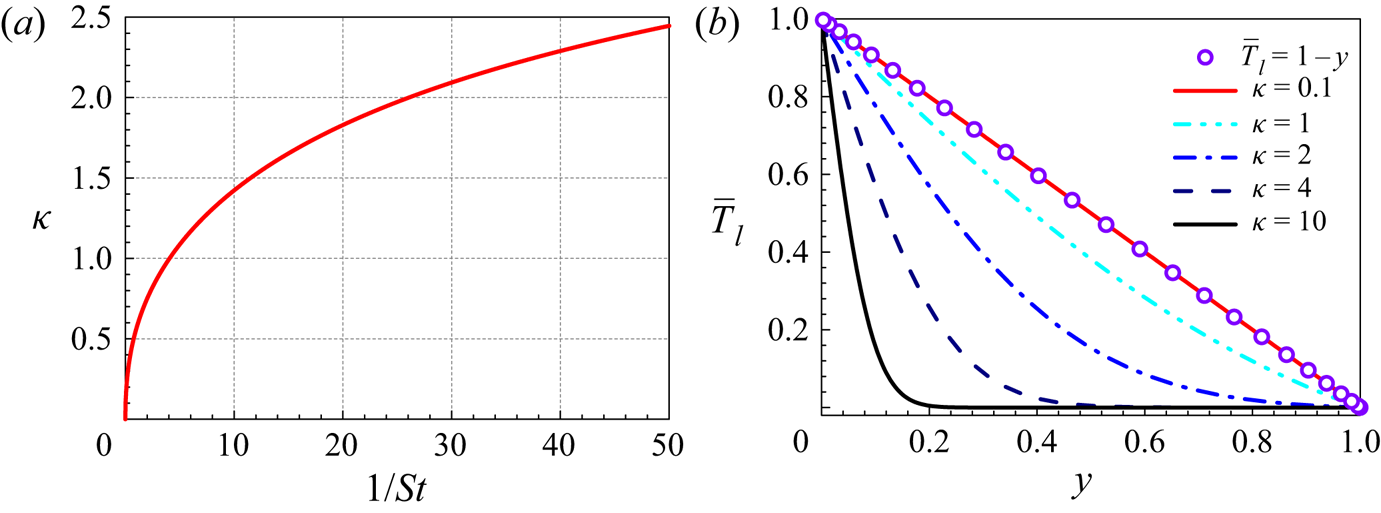
Here, we show that the time-dependent melting boundary can lead to a quasi-steady basic temperature field in the large-Stefan-number limit. We first note that, for any given St, the value of κ can be easily obtained by solving (2.24) numerically, as shown in figure 14(a). It is obvious that (2.22) is time dependent and dimensionless. Assume that, at the moment t 0, the position of the interface is at y = h 0. Note that h 0 has been chosen as our length scale. Then, for t = t 0 we obtain the dimensionless temperature in the liquid, as shown in figure 14(b). For different St, h 0 (in dimensional form) is different, but after non-dimensionalization, the thickness of the liquid at t = t 0 will always be unity. More importantly, inspecting (2.21b), it is found that for St→ $\infty$, one has ∂h/∂t = 0, which indicates that, in the large-Stefan-number limit, the depth of the liquid layer will not change with time. Looking at (2.21a), it is seen that, in this situation, the temperature in the liquid will also be independent of time.
(a) Phase-change rate as a function of Stefan number and (b) temperature in the liquid for different phase-change rates.

For simplicity, in this study we will focus on the limit of the large Stefan number. Interestingly, in this limit the temperature distribution in the liquid asymptotes to 1−y, the base state of SBS, as shown in figure 14(b). The experimental possibilities of the large-Stefan-number limit have been evaluated by Vasil & Proctor (Reference Vasil and Proctor2011). In particular, it should be noted that, in the context of subglacial plumes, the ambient water is usually within a few degrees of its melting/freezing point (Hewitt Reference Hewitt2020), which can provide a large enough Stefan number (see the definition (2.14d)).
Appendix B. Numerical method and validation
For the dynamics in the liquid, we numerically solve the eigenvalue problem, (2.29)–(2.33), along with boundary conditions, (2.34), using a spectral method based on collocation points chosen as the roots of Chebyshev polynomials (Weideman & Reddy Reference Weideman and Reddy2000). More details are given in Zhang et al. (Reference Zhang, Martinelli, Wu, Schmid and Quadrio2015).
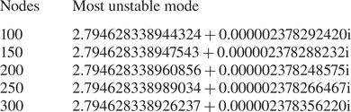
Before code validation, we have carefully checked the numerical convergence for all typical cases appearing in our calculations. In table 1 we show the most unstable modes for RB–Poiseuille flow with a phase boundary (SBS). Satisfactory convergence at 250 Chebyshev nodes is readily seen. Therefore, we use 250 nodes throughout the calculations.
Convergence check for the most unstable eigenvalue for RB–Poiseuille flow with a phase boundary (QBS). The parameters are  $\varLambda$ = 1, Ra = 28 698, k = 6.298, m = 0, Pr = 1 and Pe = 100.

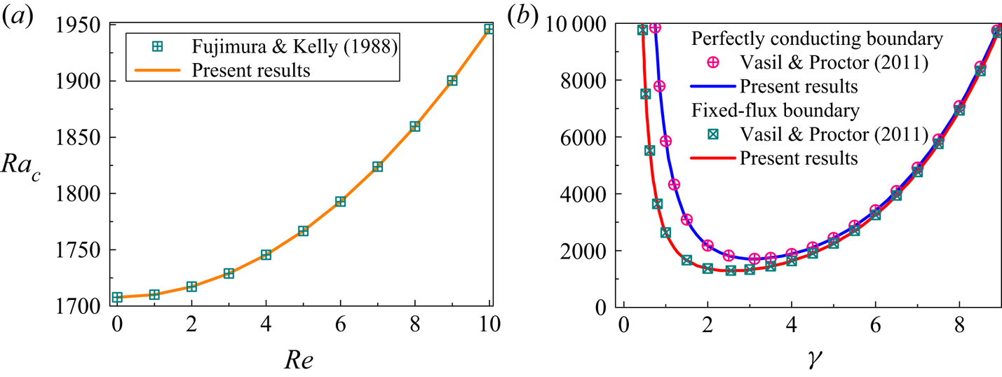
Since there exist no quantitative results for the combined effects of shear and a phase boundary on RB instability, we first partially verify our results by examining the critical Rayleigh numbers in RB–Poiseuille flow for small Reynolds numbers. In the presence of Poiseuille flow, the critical Rayleigh number Rac as a function of Reynolds number Re is shown in figure 15(a). The results of Fujimura & Kelly (Reference Fujimura and Kelly1988) are also shown for comparison. Our results match up to 5 significant digits with the results of Fujimura & Kelly (Reference Fujimura and Kelly1988).
(a) Critical Rayleigh number as a function of Re in the case of RB–Poiseuille flow. (b) Stability boundary of RB convection for different boundary conditions.

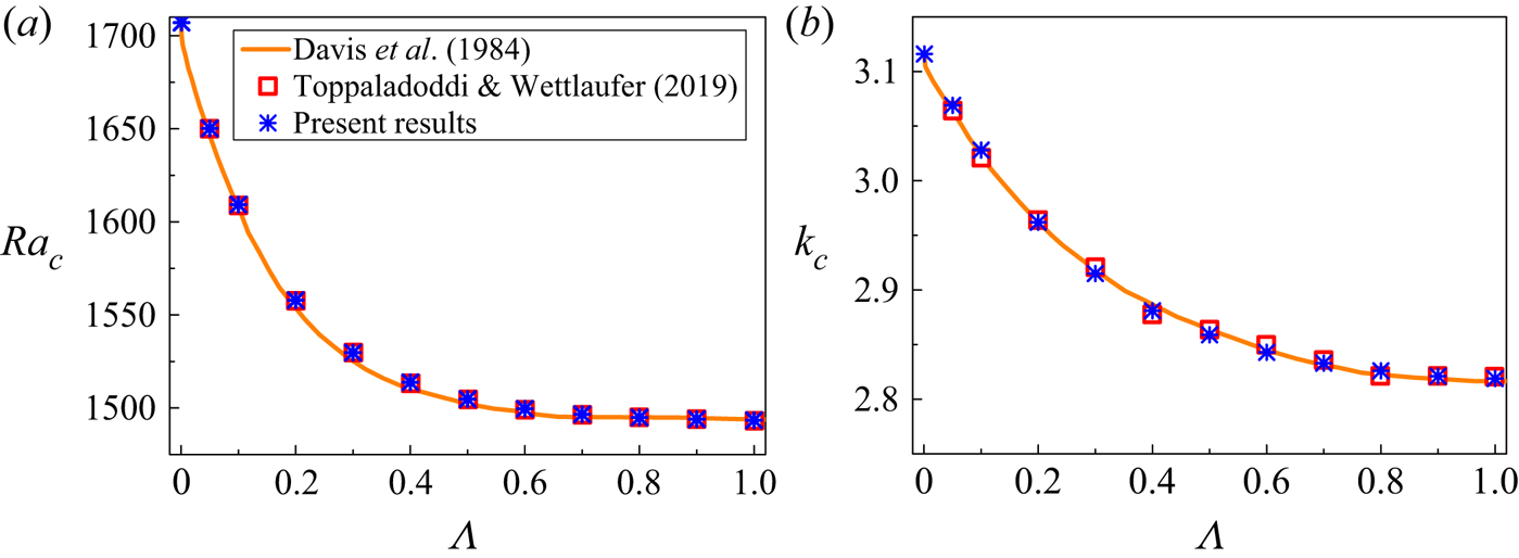
Regarding the RB instability in the presence of a phase boundary, we first examine the convective instability for QBS. Figure 15(b) shows the critical Rayleigh number as a function of wavenumber for different boundary conditions. The stability boundary of our calculation coincides with Vasil & Proctor (Reference Vasil and Proctor2011). Particularly, the stability criteria of our calculation are (1707.762, 3.116) for a perfectly conducting boundary and (1295.778, 2.552) for a fixed-flux boundary, consistent with Vasil & Proctor (Reference Vasil and Proctor2011). Comparisons of the stability analysis for SBS are made against the results of Davis et al. (Reference Davis, Müller and Dietsche1984) and Toppaladoddi & Wettlaufer (Reference Toppaladoddi and Wettlaufer2019). As shown in figures 16(a) and 16(b), with the increase of  $\varLambda$, (Rac, kc) first decrease and then asymptote to (1493, 2.815) for
 $\varLambda$ > 1. Good agreement between our results and those in Davis et al. (Reference Davis, Müller and Dietsche1984) and Toppaladoddi & Wettlaufer (Reference Toppaladoddi and Wettlaufer2019) is achieved.
Critical Rayleigh number (a) and critical wavenumber (b) for the onset of convection as functions of  $\varLambda$.

Appendix C. Instability of longitudinal, transverse and oblique rolls
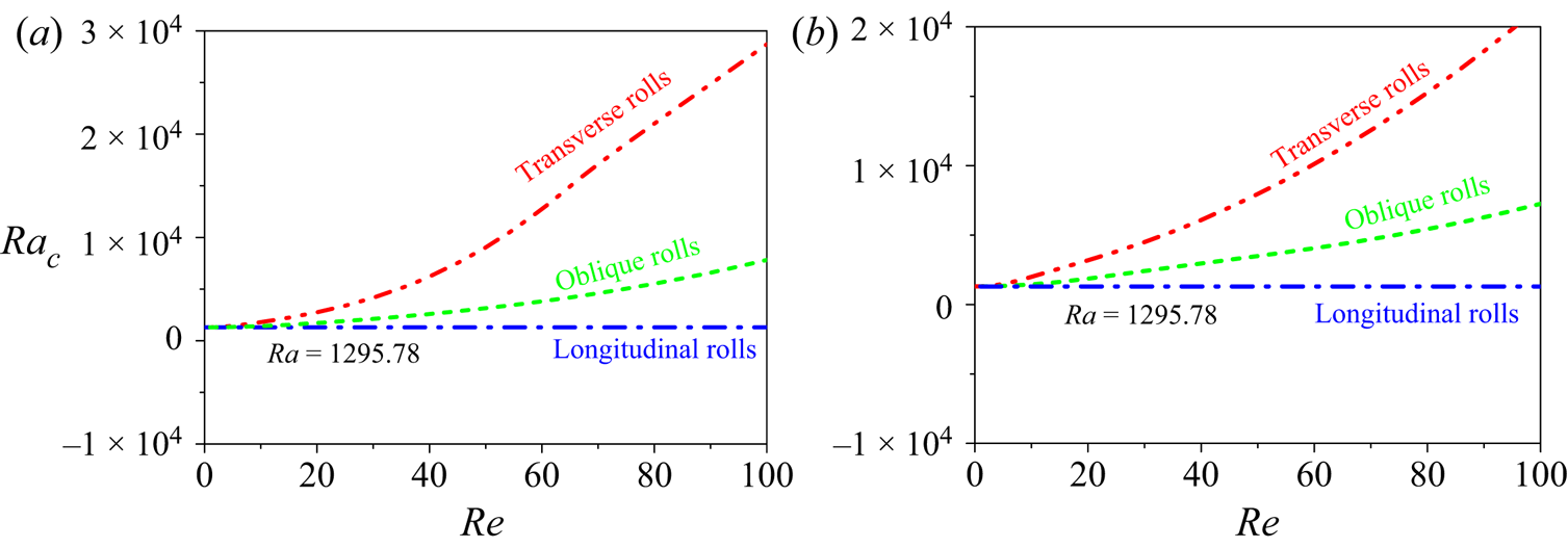
It is well known that the bifurcation of classical RB convection is symmetric, with the convection rolls arising in arbitrary orientation. In the presence of a solid–liquid interface, this symmetry remains, despite the fact that the convection threshold has changed considerably. However, the introduction of a unidirectional background shear will break the rotation symmetry of the base state so that three different modes should be distinguished: longitudinal rolls (k = 0, m > 0), transverse rolls (k > 0, m = 0) and oblique rolls (k > 0, m > 0). As mentioned before, in a system with infinite horizontal extent, longitudinal rolls are the most rapidly amplifying mode while transverse rolls are the slowest growing one, as shown in figure 17.
Stability boundaries of longitudinal, transverse and oblique rolls in the presence of a melting boundary (QBS). (a) Poiseuille flow imposed and (b) Couette flow imposed. The wavenumber of oblique rolls is k = 2.5520.5/2, m = 2.5520.5. The wavenumber of longitudinal rolls is k = 0, m = 2.552.

For simplicity, however, in this study we restrict our attention to two-dimensional motions, which means that our analysis is limited to transverse rolls (spanwise invariant), ruling out longitudinal rolls, as pointed by one of the reviewers. This consideration is meaningful due to the fact that, in a sequence of more realistic systems, one has to consider a finite spanwise domain, which can surprisingly yield a preferred mode different from the case of infinite horizontal extent. It has been confirmed that the stability of all the various rolls is a decreasing function of the spanwise extent of the rectangular channel (Luijkx et al. Reference Luijkx, Platten and Legros1981; Müller et al. Reference Müller, Lücke and Kamps1992; Kato & Fujimura Reference Kato and Fujimura2000). Moreover, if the spanwise extent is sufficiently narrow, the transverse rolls will supersede the longitudinal rolls to be the most unstable mode. For example, Kato & Fujimura (Reference Kato and Fujimura2000) found that, in a channel of identical width and height (i.e. the transverse aspect ratio is 1), transverse rolls, rather than longitudinal rolls, are the preferred mode as long as Re < 80. In the context of oceanography, the instability of transverse rolls is of great significance because transverse perturbations are found to play a vital role in the generation of basal channels underneath ice shelves (Dallaston et al. Reference Dallaston, Hewitt and Wells2015). Basal channels are ubiquitous beneath melting ice shelves, and have a profound influence on the basal melting rate, thus affecting the evolution of ice shelves on a large time scale (e.g. Dutrieux et al. Reference Dutrieux, Vaughan, Corr, Jenkins, Holland, Joughin and Fleming2013; Hewitt Reference Hewitt2020). Therefore, in this study we focus on the two-dimensional problem with m = 0.