1 Introduction
With a re-emergence of interest in hypersonic vehicle technology, there is a need for characterizing and optimizing performance. At these high speeds, laminar-to-turbulent transition is important to predict and control. Flight parameters (e.g. Mach number, unit Reynolds number, chord Reynolds number and angle of attack (AoA)), vehicle geometry (e.g. bluntness, sweep, pressure gradients and surface features) and other physical processes (e.g. high-enthalpy effects and chemical reactions) can modify either the receptivity process or the resulting pathways to transition in ways that must be explained and ultimately controlled with efficient strategies (Reed et al. Reference Reed, Perez, Kuehl, Kocian and Oliviero2015).
In order to explain the phenomenon of laminar–turbulent transition, it is important to understand the fundamental stability mechanisms that influence the behaviour of the boundary layer. There is a plethora of information about low-speed boundary layer development and transition, but there are key differences in the supersonic and hypersonic regimes that Mack (Reference Mack1984) points out. Mack describes three major differences between supersonic and subsonic two-dimensional (2D) basic state flows: the presence of a generalized inflection point, the dominance of three-dimensional (3D) viscous disturbances called ‘first modes’ (as compared with 2D viscous disturbances for the subsonic regime) and the presence of high-frequency acoustic modes. For a 2D adiabatic flat-plate boundary layer at edge Mach number greater than approximately 4, a 2D inviscid acoustic mode is generally found to be the dominant instability. This is termed the ‘second mode’, or ‘Mack mode’, and is tuned to and influenced by the thermal boundary layer. Mack modes become slightly oblique in a 3D boundary layer (Balakumar & Reed Reference Balakumar and Reed1991; Paredes et al. Reference Paredes, Perez, Reed and Theofilis2014).
A 3D geometry and non-zero AoA can result in curved streamlines and 3D basic state velocity profiles that can be highly inflectional, and thus unstable, and lead to the crossflow instability. Concerning crossflow, the past decades have seen an international effort with close collaboration among theory, computations, experiments and flight tests, resulting in the identification of important factors for subsonic, transonic and low supersonic flows (Reed & Saric Reference Reed and Saric1998; Saric, Reed & White Reference Saric, Reed and White2003). First, linear theories predict that travelling crossflow waves are more amplified than stationary waves. However, linear theories do not take into account receptivity, and it has been found that crossflow is ultra-sensitive to both leading-edge roughness and free-stream vorticity. In a flight environment, free-stream vorticity is practically non-existent, and stationary crossflow is observed due to roughness. Nonlinear effects and modal interaction play an early and important role in transition because of the presence of these stationary co-rotating vortices. These vortices distort the mean flow to include inflection points which destabilize the high-frequency secondary instabilities that rapidly break down to turbulence. As important nonlinear effects occur early on, a nonlinear approach such as a nonlinear parabolized stability equation (NPSE) (Herbert Reference Herbert1997) or direct numerical simulation (DNS) approach is necessary.
Recently, simple 3D geometries (yawed straight circular cones and elliptic cones) have been studied to provide insight into the stability and transition of hypersonic vehicles. As a testimony to the complexity of the problem, considerable uncertainty still exists within the community related to the roles of stationary and travelling crossflow and Mack modes, effects of spanwise-varying basic states, roles of roughness/receptivity, secondary instabilities and breakdown. Many experiments have been completed and indicate that the basic stability mechanisms in 3D boundary layers consist of multiple modes, i.e. first modes, second modes and stationary and travelling crossflow (Juliano & Schneider Reference Juliano and Schneider2010; Chynoweth et al. Reference Chynoweth, Ward, Greenwood, Mckiernan, Fisher and Schneider2014; Munoz, Heitmann & Radespiel Reference Munoz, Heitmann and Radespiel2014; Borg, Kimmel & Stanfield Reference Borg, Kimmel and Stanfield2015; Ward, Henderson & Schneider Reference Ward, Henderson and Schneider2015; Craig & Saric Reference Craig and Saric2016; Sweeney et al. Reference Sweeney, Chynoweth, Edelman and Schneider2016). Recent DNS, parabolized stability equations (PSE; both linear (LPSE) and nonlinear (NPSE)) and global methods (Choudhari et al. Reference Choudhari, Chang, Jentink, Li, Berger, Candler and Kimmel2009; Balakumar & Owens Reference Balakumar and Owens2010; Gosse, Kimmel & Johnson Reference Gosse, Kimmel and Johnson2010; Paredes et al. Reference Paredes, Theofilis, Rodriguez and Tendero2011; Theofilis Reference Theofilis2011; Kuehl, Perez & Reed Reference Kuehl, Perez and Reed2012; Paredes Reference Paredes2014; Paredes & Theofilis Reference Paredes and Theofilis2014; Oliviero et al. Reference Oliviero, Kocian, Moyes and Reed2015) are providing great insight, and computational efforts indicate how important grid convergence is for the basic state of 3D geometries (Dinzl & Candler Reference Dinzl and Candler2015).
The purpose of this paper is to provide secondary instability analysis of stationary crossflow vortices on a hypersonic yawed straight circular cone. The remainder of the paper is organized in the following manner. The next section presents the conditions of the yawed straight circular cone studied and various flow variable contours of its laminar undisturbed basic state. Then the discussion shifts to the stability calculations and techniques used to do secondary instability analysis. The following section discusses key concepts from low-speed crossflow secondary instability findings and from hypersonic second mode analysis, which are useful in helping identify various unstable modes captured in the present results. Then, a path and the initial conditions are chosen, based on the Mach 6 Quiet Tunnel experiment at Texas A&M University, and primary and secondary instability analysis is completed. The results are then compared with the experimental findings of Craig & Saric (Reference Craig and Saric2016). Then, primary and secondary instability analysis is performed for a similar path with the initial conditions of the Ward et al. (Reference Ward, Henderson and Schneider2015) experiment and comparisons are made. Finally, putting all the results together, the instabilities are compared to those for an incompressible swept wing and conclusions are offered.
2 Basic state geometry
The geometry considered in this work is the yawed straight circular cone. As such, a plethora of experimental and computational literature exists on the subject. Balakumar & Owens (Reference Balakumar and Owens2010) considered DNS solutions of roughness-induced stability on a
 $7^{\circ }$
half-angle straight cone yawed to
 $6^{\circ }$
AoA at Mach 6, and considered LPSE analysis of the same case for a clean (no-roughness) basic state. Both the DNS and the LPSE demonstrate the dominance of crossflow instability away from the leeward and windward symmetry planes. In the Texas A&M Mach 6 Quiet Tunnel, Craig & Saric (Reference Craig and Saric2016) conducted detailed measurements within the boundary layer of the crossflow instability on the same geometry. Note that their model was at
 $5.6^{\circ }$
AoA due to blockage concerns. Furthermore, Ward et al. (Reference Ward, Henderson and Schneider2015) conducted detailed measurements at the wall with Kulite and PCB sensors of the same geometry at
 $6^{\circ }$
AoA at the Boeing/AFOSR Mach 6 Quiet Tunnel at Purdue University.
The cone model currently being studied has a nose radius of
 $0.05$
mm and a half-angle of
 $7^{\circ }$
and is at a
 $6^{\circ }$
AoA. The model is
 $0.508$
m (
 $20$
in.) in length. Conditions for the basic state calculation consisted of free-stream Mach number
 $M_{\infty }=6$
, unit Reynolds number based on free-stream conditions
 $Re^{\prime }=10.09\times 10^{6}~\text{m}^{-1}$
, free-stream temperature
 $T_{\infty }=53.42$
K and free-stream absolute pressure
 $P_{\infty }=611.38$
Pa abs.
For most stability analyses, the total flow is separated into a basic state and a disturbance. The basic state is a highly resolved steady laminar solution to the compressible Navier–Stokes equations. The flow over the considered geometry is computed using the Data Parallel Line Relaxation (DPLR) NASA computational fluid dynamics (CFD) code (Wright Reference Wright2009). The grid size used in the calculation of the basic state contains 209 points along the axial direction, 333 wall-normal and 325 azimuthally. The symmetry of the problem at hand is exploited to reduce the computational domain to one half. A no-slip, constant
 $T_{w}=300$
K wall boundary condition was applied on the cone surface. All computations were performed assuming air as an ideal gas using Sutherland’s law for viscosity and a constant Prandtl number
 $Pr=0.72$
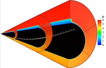
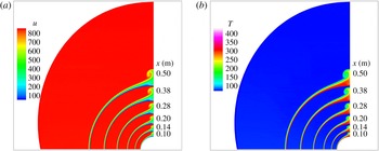
. The basic state Mach contour solution can be seen in figure 1. The vortex paths used for stability analysis are included on the surface and will be discussed further in later sections. Also, more detailed contours of
 $u$
(
 $\text{m}~\text{s}^{-1}$
) and
 $T$
(K) at various axial slices are shown in figure 2. These slices focus on the leeward side of the yawed cone in order to show the development of the mushroom structure downstream.
Mach contour: undisturbed laminar basic state solution computed using DPLR. The solid white line is vortex path to compare with Craig & Saric (Reference Craig and Saric2016) and dashed white line is vortex path to compare with Ward et al. (Reference Ward, Henderson and Schneider2015).

Axial contour slices of
 $u$
(
 $\text{m}~\text{s}^{-1}$
) and
 $T$
(K) on leeward side of undisturbed laminar basic state solution computed using DPLR. The axial locations are
 $x=0.10$
, 0.14, 0.20, 0.28, 0.38 and 0.50 m.

3 Stability calculations
To model disturbance growth within the boundary layer, different methods may be applied. This work utilizes linear stability theory (LST), NPSE and LST based on 2D partial differential equations (PDEs), also known as spatial BiGlobal (SBG) theory, for secondary stability analysis, all including the streamwise and azimuthal curvature terms. They are accounted for by a transformation to a general orthogonal curvilinear coordinate system with the proper metrics that are based on the streamwise and azimuthal radii of curvature. In each case, each flow variable is decomposed into a steady basic state quantity, upon which a disturbance is to be superposed, and the unsteady disturbance itself. This superposition is substituted into the governing equations to yield the disturbance equations, which describe the evolution of the disturbance. Each method considers a different solution form of the disturbance. The LST and NPSE methods as implemented in EPIC, a Texas A&M University developed code, are described in detail by Oliviero et al. (Reference Oliviero, Kocian, Moyes and Reed2015). Summarizing, for flow variables represented by
 $\unicode[STIX]{x1D719}=[u,v,w,T,\unicode[STIX]{x1D70C}]^{\text{T}}$
, LST (Mack Reference Mack1984) assumes two homogeneous spatial directions and small disturbance amplitudes (local and linear solutions). The disturbance quantities are modelled as an eigenvalue problem with a disturbance of the form
 $$\begin{eqnarray}\displaystyle \unicode[STIX]{x1D719}_{LST}^{\prime }(\unicode[STIX]{x1D709},\unicode[STIX]{x1D702},\unicode[STIX]{x1D701},t)=\hat{\unicode[STIX]{x1D719}}(\unicode[STIX]{x1D702})\exp [\text{i}(\unicode[STIX]{x1D6FC}\unicode[STIX]{x1D709}+\unicode[STIX]{x1D6FD}\unicode[STIX]{x1D701}-\unicode[STIX]{x1D714}t)]+\text{c.c.} & & \displaystyle\end{eqnarray}$$
Here
 $\unicode[STIX]{x1D709}$
,
 $\unicode[STIX]{x1D702}$
and
 $\unicode[STIX]{x1D701}$
are the body-fitted marching, wall-normal and mutually perpendicular coordinates, respectively;
 $u$
,
 $v$
and
 $w$
are the corresponding velocity components in those directions; and c.c. represents the complex conjugate.
When solving the PSE equations (Herbert Reference Herbert1997), the boundary layer is assumed to grow slowly in the disturbance-propagation direction and second derivatives in that direction are neglected, nearly parabolizing the stability equations and allowing a marching solution. In order to solve a marching solution, a predefined path is required. Also, the PSE equations assume a spanwise-invariant mean flow. For LPSE, a single mode is marched without nonlinear interactions. In this paper, NPSE is used to capture large amplitudes and nonlinearities of disturbances. The disturbances are assumed to have the form
 $$\begin{eqnarray}\displaystyle \unicode[STIX]{x1D719}_{NPSE}^{\prime }(\unicode[STIX]{x1D709},\unicode[STIX]{x1D702},\unicode[STIX]{x1D701},t)=\mathop{\sum }_{n=-N}^{N}\mathop{\sum }_{k=-K}^{K}\left[\frac{A_{0_{n,k}}}{2}\underbrace{\hat{\unicode[STIX]{x1D719}}_{n,k}(\tilde{\unicode[STIX]{x1D709}},\unicode[STIX]{x1D702})}_{\text{shape}}\underbrace{A(\unicode[STIX]{x1D709})\text{e}^{\text{i}(k\unicode[STIX]{x1D6FD}(\tilde{\unicode[STIX]{x1D709}})\unicode[STIX]{x1D701}-n\unicode[STIX]{x1D714}t)}}_{\text{wave}}\right]+\text{c.c.}, & & \displaystyle\end{eqnarray}$$
where
 $A_{0_{n,k}}$
is the initial amplitude of the individual disturbance modes (mode plus complex conjugate),
 $A(\unicode[STIX]{x1D709})=\text{e}^{\text{i}\int \unicode[STIX]{x1D6FC}_{n,k}(\tilde{\unicode[STIX]{x1D709}})\,\text{d}\unicode[STIX]{x1D709}}$
is the amplitude function, and
 $\unicode[STIX]{x1D6FC}_{n,k}(\tilde{\unicode[STIX]{x1D709}})$
and
 $\unicode[STIX]{x1D6FD}(\tilde{\unicode[STIX]{x1D709}})$
are the complex marching-direction and spanwise wavenumbers, respectively, which are assumed to be slowly varying in the marching direction. Owing to the slowly varying nature of
 $\unicode[STIX]{x1D6FD}(\tilde{\unicode[STIX]{x1D709}})$
, its derivatives in the
 $\unicode[STIX]{x1D709}$
direction are small and not included in the PSE calculations for this analysis. The subscripts
 $n$
and
 $k$
correspond to integer multiples of the primary disturbance frequency (
 $\unicode[STIX]{x1D714}$
) and spanwise wavenumber (
 $\unicode[STIX]{x1D6FD}(\tilde{\unicode[STIX]{x1D709}})$
), respectively, with each mode having its own unique combination. For this paper,
 $\unicode[STIX]{x1D6FD}(\tilde{\unicode[STIX]{x1D709}})=m(\tilde{\unicode[STIX]{x1D709}})/R(\unicode[STIX]{x1D709})$
, where
 $m$
is defined as the
 $\unicode[STIX]{x1D701}$
-direction wavenumber (number of stationary crossflow waves in the
 $\unicode[STIX]{x1D701}$
direction) and
 $R$
is the radius of curvature in the
 $\unicode[STIX]{x1D701}$
direction.
In the present study of secondary instabilities (disturbances) of nonlinearly distorted stationary crossflow (basic state), the
 $\unicode[STIX]{x1D701}$
-direction variations of the basic state are of the same order as the wall-normal variations. The analysis of such a modified basic state is only accessible by multi-dimensional stability analysis. SBG analysis is the 2D analogue of the classic spatial LST. Here, two inhomogeneous directions are resolved simultaneously on a plane, while the third direction is considered locally homogeneous or quasi-parallel. The grid for SBG analysis clusters near the wall in the wall-normal direction and uses Fourier collocation with equally spaced points in the spanwise direction. This implies periodic boundary conditions in the spanwise direction (Paredes et al.
Reference Paredes, Gosse, Theofilis and Kimmel2016). A complete review of multi-dimensional and global stability analysis techniques is given by Theofilis (Reference Theofilis2011). A code developed at Universidad Politécnica de Madrid is used presently; details are given by Paredes (Reference Paredes2014) and Paredes & Theofilis (Reference Paredes and Theofilis2014). The disturbance quantities take the form
 $$\begin{eqnarray}\displaystyle \unicode[STIX]{x1D719}_{SBG}^{\prime }(\unicode[STIX]{x1D709},\unicode[STIX]{x1D702},\unicode[STIX]{x1D701},t)=\hat{\unicode[STIX]{x1D719}}(\unicode[STIX]{x1D702},\unicode[STIX]{x1D701})\exp [\text{i}(\unicode[STIX]{x1D6FC}\unicode[STIX]{x1D709}-\unicode[STIX]{x1D714}t)]+\text{c.c.} & & \displaystyle\end{eqnarray}$$
Applying SBG to the present problem, it is necessary to include all basic state velocity components (
 $\bar{u}^{\ast },\bar{v}^{\ast },\bar{w}^{\ast }$
), as well as the thermodynamic variables
 $\bar{T}^{\ast }$
and
 $\bar{\unicode[STIX]{x1D70C}}^{\ast }$
, in the calculations. The nonlinearly distorted basic state (modified basic state) takes the form
 $$\begin{eqnarray}\displaystyle \bar{\unicode[STIX]{x1D719}}^{\ast }(\tilde{\unicode[STIX]{x1D709}},\unicode[STIX]{x1D702},\unicode[STIX]{x1D701})=\bar{\unicode[STIX]{x1D719}}(\tilde{\unicode[STIX]{x1D709}},\unicode[STIX]{x1D702},\unicode[STIX]{x1D701})+\unicode[STIX]{x1D719}_{NPSE}^{\prime }(\tilde{\unicode[STIX]{x1D709}},\unicode[STIX]{x1D702},\unicode[STIX]{x1D701}), & & \displaystyle\end{eqnarray}$$
where
 $\bar{\unicode[STIX]{x1D719}}$
is the dimensional steady laminar flow over the geometry and
 $\unicode[STIX]{x1D719}_{NPSE}^{\prime }$
is the dimensional NPSE wave formulation disturbance (3.2). Since these calculations are for stationary crossflow, there is no time dependence in the modified basic state. Also, as the marching path is in the direction of the stationary crossflow vortex and saturation occurs once nonlinearities set in, the modified basic state is assumed to be slowly varying in
 $\unicode[STIX]{x1D709}$
. The dimensional total flow is given by
 $$\begin{eqnarray}\displaystyle \unicode[STIX]{x1D719}(\unicode[STIX]{x1D709},\unicode[STIX]{x1D702},\unicode[STIX]{x1D701},t)=\bar{\unicode[STIX]{x1D719}}^{\ast }(\tilde{\unicode[STIX]{x1D709}},\unicode[STIX]{x1D702},\unicode[STIX]{x1D701})+\unicode[STIX]{x1D719}_{SBG}^{\prime }(\unicode[STIX]{x1D709},\unicode[STIX]{x1D702},\unicode[STIX]{x1D701},t), & & \displaystyle\end{eqnarray}$$
where
 $\bar{\unicode[STIX]{x1D719}}^{\ast }$
is the dimensional modified basic state (3.4) and
 $\unicode[STIX]{x1D719}_{SBG}^{\prime }$
is the dimensional SBG disturbance (3.3).
4 Travelling crossflow, secondary instability and second mode key concepts for analysis
4.1 Low-speed three-dimensional basic states
At low speeds, travelling crossflow is a primary instability in low-amplitude regions, but in nonlinear regions, the travelling crossflow becomes modulated (Fischer & Dallmann Reference Fischer and Dallmann1991). This alteration of the original travelling crossflow has been cited as a modulated travelling crossflow (White & Saric Reference White and Saric2005; Li & Choudhari Reference Li and Choudhari2011) (see their figure 7 and their figure 6, respectively), which is the expression used in this paper, and a type-III secondary instability (Bonfigli & Kloker Reference Bonfigli and Kloker2007) (see their figure 11b). The travelling crossflow interacts with the stationary crossflow; however, the shape of the stationary crossflow is unaffected by this interaction (Fischer & Dallmann Reference Fischer and Dallmann1991). The travelling crossflow is originally concentrated near the wall (Malik, Li & Chang Reference Malik, Li and Chang1994). Once the disturbances become large and nonlinear, the travelling crossflow is lifted by the vortex into the low-momentum upwelling of the wave (White & Saric Reference White and Saric2005). Finally, secondary instability analysis can result in multiple travelling crossflow modes, which can have different frequency ranges and growth rates (Malik, Li & Chang Reference Malik, Li and Chang1996).
Also, there are two different classifications of a secondary instability, a type-I and a type-II instability (Malik et al.
Reference Malik, Li and Chang1996). Type I follows the extrema of the
 $\unicode[STIX]{x1D701}$
gradient of the modified
 $\unicode[STIX]{x1D709}$
component of the flow,
 $\unicode[STIX]{x2202}u/\unicode[STIX]{x2202}\unicode[STIX]{x1D701}$
, and is typically in the low-frequency spectrum. An approximation at low speeds of the type-I instability can be calculated via the equation (Craig & Saric Reference Craig and Saric2016)
 $$\begin{eqnarray}\displaystyle F=\frac{U_{e}}{2\unicode[STIX]{x1D6FF}}. & & \displaystyle\end{eqnarray}$$
For this paper,
 $\unicode[STIX]{x1D6FF}$
is the wall-normal distance for which the
 $\unicode[STIX]{x1D701}$
-direction-averaged
 $u$
velocity of the modified basic state profile reaches
 $99\,\%$
of the edge value. Type II consists of the extrema of the wall-normal gradient,
 $\unicode[STIX]{x2202}u/\unicode[STIX]{x2202}\unicode[STIX]{x1D702}$
, and is typically in the higher-frequency spectrum. Furthermore, at low speeds, complete analysis of crossflow-induced secondary instabilities has been performed (White & Saric Reference White and Saric2005).
According to Malik et al. (Reference Malik, Li, Choudhari and Chang1999), when the stationary crossflow amplitudes are of the order of the basic state quantities, there can exist as many as seven unstable modes that most likely are type I, type II or a combination of both secondary instabilities. Furthermore, it has been explained before that multiple peaks in the growth-rate plot can combine into a single mode (Malik et al. Reference Malik, Li, Choudhari and Chang1999). Also, the crossing of modes with other modes is called modal degeneracy, a concept discussed in more depth by Koch (Reference Koch1992). This might provide more insight into the overlapping of modes at a frequency and growth rate.
4.2 High-speed basic states
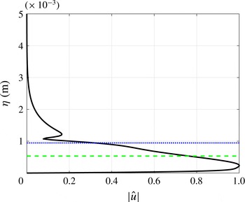
Additionally, for high-speed flows, a second mode disturbance (Mack Reference Mack1984) may be unstable in the original undisturbed laminar-flow basic state as well as in the modified basic state (such as is given by (3.4)). A second mode has unique characteristics. As shown in figure 3, the
 $|\hat{u} |$
mode shape has two peaks, one close to the wall below the relative sonic line and one slightly above the critical layer. The critical layer is defined as the location in the boundary layer at which the velocity of the disturbance (phase speed) is equal to the mean velocity of the local flow field (Mack Reference Mack1984).
Generic LST second mode, lines of
 $|\hat{u} |$
mode shape (solid black), critical layer (dotted blue) and relative sonic line (dashed green).

5 Experimental and computational overview
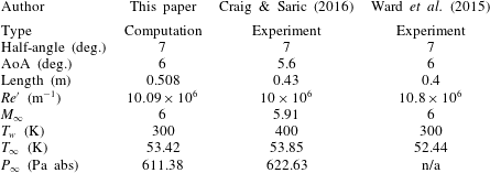
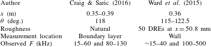
Secondary instabilities have recently been studied in the Mach 6 Quiet Tunnel at Texas A&M University (Craig & Saric Reference Craig and Saric2016) and the Boeing/AFOSR Mach 6 Quiet Tunnel at Purdue University (Ward et al. Reference Ward, Henderson and Schneider2015) for the yawed straight circular cone. The experiments were completed in a strong 3D boundary layer region that leads to highly nonlinear and large-amplitude stationary crossflow and secondary instabilities of that crossflow vortex. This gives a basis of where to focus computations. The conditions of each case are listed in table 1. There are a few variations in the flow conditions between the quiet wind tunnel experiments and the computations performed. The most noticeable difference is the wall temperature from the Craig & Saric (Reference Craig and Saric2016) experiment (400 K) and the computations (300 K). Work done by Lekoudis (Reference Lekoudis1980) and Mack (Reference Mack1980) explained that wall temperature has a mild stabilizing effect on the stationary crossflow instability in 3D boundary layers. Furthermore, Sznitko (Reference Sznitko1993) concluded that the effectiveness of wall cooling decreases with a stronger stationary crossflow instability. Finally, it has been explained by Meier & Schnerr (Reference Meier and Schnerr1996) that wall cooling stabilizes crossflow, but it is minimal as the inflection point of the crossflow mean velocity profile is located towards the edge of the boundary layer. Based on this past work, the wall temperature difference between Craig & Saric (Reference Craig and Saric2016) and the computations should only minimally effect the stability calculations for stationary crossflow. However, there could be an effect on the convective instability modes whose frequencies tend to scale with the boundary layer thickness, so meaningful qualitative comparisons will be made in these cases.
Comparison of conditions from this work, Craig & Saric (Reference Craig and Saric2016) and Ward et al. (Reference Ward, Henderson and Schneider2015) for a straight yawed circular cone.

To do the secondary instability analysis, an unperturbed laminar basic state and primary NPSE disturbances are superposed to create a new modified basic state (3.4). NPSE analysis requires a predefined marching path. Both experiments visualized stationary crossflow vortices, and the appropriate marching path has previously been shown to be a vortex path (Oliviero et al.
Reference Oliviero, Kocian, Moyes and Reed2015). The vortex path is calculated from the undisturbed basic state using the inflection-point method, where the path is locally aligned such that the generalized inflection point of the
 $\bar{\unicode[STIX]{x1D70C}}\bar{w}$
mass flux occurs at
 $\bar{\unicode[STIX]{x1D70C}}\bar{w}=0$
. Furthermore, EPIC includes a
 $\unicode[STIX]{x1D701}$
-direction-wavenumber variation in the downstream direction along the vortex path (see Oliviero et al.
Reference Oliviero, Kocian, Moyes and Reed2015). This downstream variation was modelled solely from consideration of the undisturbed basic state and is verified from studying the DNS solution by Balakumar & Owens (Reference Balakumar and Owens2010). It is assumed that the number of stationary crossflow waves remains constant between neighbouring computational vortex paths. As the vortex paths develop downstream, the distance between them expands or narrows. This change in distance, coupled with the vortex-path direction, is used to determine the local effective
 $\unicode[STIX]{x1D701}$
-direction wavenumber. The new modified basic state is the input to the BiGlobal method and secondary instabilities are sought. Table 2 shows the findings from the experiments of Craig & Saric (Reference Craig and Saric2016) and Ward et al. (Reference Ward, Henderson and Schneider2015) that will be the basis for comparisons. The experiments are quite different from each other, with different roughness distributions and heights, measurement locations and frequency ranges capable of being observed, and it is important to analyse both.
List of results from Craig & Saric (Reference Craig and Saric2016) and Ward et al. (Reference Ward, Henderson and Schneider2015) for a straight yawed circular cone (DREs = discrete roughness elements).

6 Craig & Saric (Reference Craig and Saric2016) experimental conditions
 $-$
natural surface roughness

6.1 Primary instability analysis
NPSE analysis requires an initial condition with a certain initial amplitude, which is then marched downstream along a prescribed path resolving the fundamental mode(s), the mean flow distortion (MFD), the harmonics and their complex conjugates. Craig & Saric (Reference Craig and Saric2016) provide hot-wire measurements through the boundary both radially and azimuthally at multiple downstream positions,
 $x=0.35{-}0.39$
m, and centred at an azimuthal angle,
 $\unicode[STIX]{x1D703}=118^{\circ }$
, from the windward plane. The first step in the present analysis is to determine a vortex path or paths passing through the experimental locations of interest. The basic state is 3D in nature with curved vortex paths; a given vortex path actually intersects
 $\unicode[STIX]{x1D703}=118^{\circ }$
at a single axial location. Using NPSE, Oliviero et al. (Reference Oliviero, Kocian, Moyes and Reed2015) computed and analysed stationary crossflow over multiple paths that intersect the various (
 $x,\unicode[STIX]{x1D703}$
) locations of the Craig & Saric (Reference Craig and Saric2016) experiment. In the present work, the focus is on a single path that passes through the location
 $x=0.38$
m at
 $\unicode[STIX]{x1D703}=118^{\circ }$
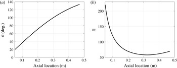
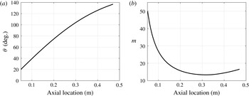
. There was little difference found in comparing the present NPSE results to those of Oliviero et al. (Reference Oliviero, Kocian, Moyes and Reed2015), attributable to the fact that the streamwise and azimuthal distances over which the experimental measurements were taken was small. The vortex path computed for this analysis is shown in figure 4(a).
The Craig & Saric (Reference Craig and Saric2016) cone is polished with no artificially added roughness elements and the root-mean-square (r.m.s.) roughness height is
 $2.15~\unicode[STIX]{x03BC}\text{m}$
. To model the
 $\unicode[STIX]{x1D701}$
-direction-wavenumber variation, the ratio of the local value to the initial value is predicted from the basic state at each marching position along the vortex path as described before. Then all that is needed is the initial value. For this case, it is assumed that all
 $\unicode[STIX]{x1D701}$
-direction wavenumbers are initially present in the natural surface roughness, and LPSE solutions are conducted along the vortex path to determine the initial
 $\unicode[STIX]{x1D701}$
-direction wavenumber leading to the maximum amplification downstream at the measurement location. The
 $\unicode[STIX]{x1D701}$
-direction-wavenumber variation is shown in figure 4(b). Craig & Saric (Reference Craig and Saric2016) provide the number of stationary crossflow waves in the
 $\unicode[STIX]{x1D703}$
direction, so it is necessary to transform it to the
 $\unicode[STIX]{x1D701}$
direction to compare with the computations. This value is locally approximately
 $m=60$
for both the present computations and the experiment at the (
 $x=0.38$
m,
 $\unicode[STIX]{x1D703}=118^{\circ }$
) location. A corresponding initial
 $m=220$
at
 $x=0.05$
m is predicted by our method for the computational vortex path, translating to an initial wavelength of approximately
 $0.20$
mm. The
 $\unicode[STIX]{x1D701}$
-direction wavenumber technique gives results consistent with the DNS solution of Balakumar & Owens (Reference Balakumar and Owens2010).
(a) Vortex path evolution of angle from windward plane; intersects
 $118^{\circ }$
at
 $0.38$
m. (b) The
 $\unicode[STIX]{x1D701}$
-direction-wavenumber (
 $m$
) variation at different axial locations; intersects
 $m=60$
at
 $x=0.38$
m.

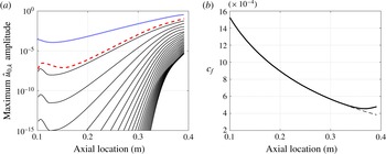
(a) Maximum
 $\hat{u} _{0,k}$
amplitude for fundamental mode (
 $k=1$
; dotted blue line), MFD (
 $k=0$
; dashed red line) and
 $23$
harmonics (
 $k=2{-}24$
; solid black lines) of stationary crossflow modes, initialized at
 $x=0.1$
m with
 $\hat{u} _{0,1}$
amplitude of
 $1.5\times 10^{-4}$
on fundamental mode. (b) Skin friction coefficient evolution of basic state (dashed line) and basic state with MFD (solid line).

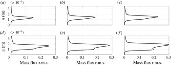
Next, an initial amplitude for the stationary crossflow was not available for the Craig & Saric (Reference Craig and Saric2016) experiment, so this quantity was varied in the computations until the resulting downstream mass flux contours, as well as the mass flux r.m.s. value compared closely with the experimental results (Oliviero et al.
Reference Oliviero, Kocian, Moyes and Reed2015). The maximum
 $\hat{u} _{0,k}$
amplitudes, normalized by the
 $\unicode[STIX]{x1D709}$
-direction edge speed
 $U_{e}$
at the initial axial location, and skin friction plots for the full NPSE calculation (3.2) are shown in figure 5(a,b), respectively. The individual complex-mode
 $\hat{u} _{0,1}$
amplitude was initialized at
 $1.5\times 10^{-4}$
(note that the NPSE wave formulation (3.2) includes the initial disturbance amplitude,
 $A_{0_{n,k}}/2$
, resulting in
 $A_{0_{0,1}}=3\times 10^{-4}$
), and its shape was provided by LST, at an axial location of
 $x=0.1$
m. As the NPSE simulation marches closer to the back of the cone, the amplitudes of the harmonics approach the same order as the basic state quantities and it is important to include enough harmonics to resolve the disturbances completely; this case uses 25 modes, i.e. the fundamental mode, the MFD and
 $23$
superharmonics. Figure 6 shows the development of the
 $x$
component of the mass flux of the total flow (basic state plus disturbance) at different downstream locations and figure 7 shows the development of the
 $x$
component of the mass flux r.m.s. (Oliviero et al.
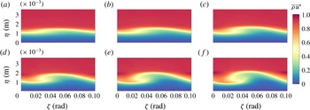
Reference Oliviero, Kocian, Moyes and Reed2015). The basis for figures 6 and 7 originate in Oliviero et al. (Reference Oliviero, Kocian, Moyes and Reed2015), in which stationary crossflow over multiple paths that intersect the Craig & Saric (Reference Craig and Saric2016) measurement locations are computed and a detailed comparison is presented there. In summary, as the stationary crossflow wave grows downstream, a rollover towards the windward plane develops and a second lobe within the mass flux r.m.s. also develops.
Isocontours of modified basic state
 $x$
component of the mass flux,
 $\bar{\unicode[STIX]{x1D70C}}\bar{u}^{\ast }$
(3.4), at (a)
 $x=0.34$
m, (b)
 $x=0.35$
m, (c)
 $x=0.36$
m, (d)
 $x=0.37$
m, (e)
 $x=0.38$
m and (f)
 $x=0.39$
m.

Mass flux r.m.s. shape of flow field in figure 6 at (a)
 $x=0.34$
m, (b)
 $x=0.35$
m, (c)
 $x=0.36$
m, (d)
 $x=0.37$
m, (e)
 $x=0.38$
m and (f)
 $x=0.39$
m.

6.2 Secondary instability analysis
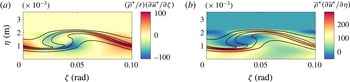
To help determine if the large-amplitude stationary crossflow achieved from the NPSE is conducive to secondary instabilities, an inflection point calculation of the most developed slice was completed. As discussed earlier, secondary instabilities typically follow the trends of the
 $\unicode[STIX]{x1D701}$
-direction and wall-normal gradients. The
 $\unicode[STIX]{x1D701}$
-direction and wall-normal gradients at
 $x=0.39$
m can be seen in figure 8, where the left contour would depict the type I, concentrating on the shoulder, and the right contour would depict the type II, concentrating on the crest or trough. Note here that the generalized gradients are used.
Five isolines (solid black) of
 $\bar{\unicode[STIX]{x1D70C}}\bar{u}^{\ast }$
and isocontours at
 $x=0.39$
m of gradients (a)
 $(\bar{\unicode[STIX]{x1D70C}}^{\ast }/r)(\unicode[STIX]{x2202}\bar{u}^{\ast }/\unicode[STIX]{x2202}\unicode[STIX]{x1D701})$
and (b)
 $\bar{\unicode[STIX]{x1D70C}}^{\ast }(\unicode[STIX]{x2202}\bar{u}^{\ast }/\unicode[STIX]{x2202}\unicode[STIX]{x1D702})$
.

To ensure that the BiGlobal instability results are converged, high-fidelity modified basic states were input into the BiGlobal code and the BiGlobal instability grid was varied in resolution until numerical convergence was achieved (the eigenmode is converged up to eight significant digits). As the primary crossflow wave develops, more points in the
 $\unicode[STIX]{x1D701}$
and wall-normal directions are required.
BiGlobal instabilities and LST were calculated at multiple axial locations in front of this developed crossflow slice along the vortex path from
 $x=0.20$
m through
 $x=0.39$
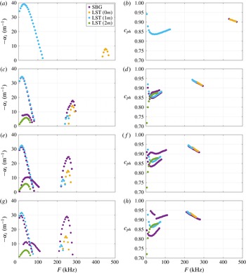
m. While SBG is applied to (3.4), the LST results are generated from the unperturbed laminar flow on the cone and are provided as guidance to see if the travelling crossflow and second mode instability exist for the modified basic state in addition to secondary instabilities. The phase speeds and growth rates of unstable modes are observed in the spectra for a broad frequency band,
 $F\in (0,500)$
kHz. Slices at
 $x=0.20{-}0.33$
m show how instabilities predicted by the BiGlobal analysis begin to deviate from LST (figure 9) and become more unstable at each axial location. The LST and SBG results are the same at
 $x=0.20$
m, as expected. It is important to note that the LST results differentiate an oblique second mode from a second mode, whereas the BiGlobal results do not differentiate them. Therefore, in order to be consistent and be able to separate modes in the SBG method, the
 $\unicode[STIX]{x1D709}$
component of the phase speeds are matched, where this component of the phase speed is calculated by
 $c_{ph}=\unicode[STIX]{x1D714}/\unicode[STIX]{x1D6FC}_{r}$
. The slices from
 $x=0.34$
m through
 $x=0.39$
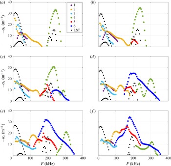
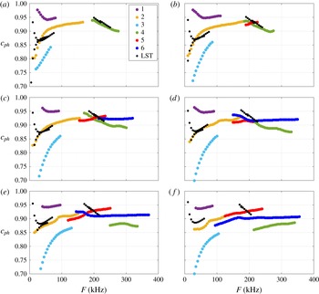
m show the development of the growth rates of six unstable modes and the LST unstable modes (figure 10). The modified basic state supports unstable travelling crossflow and second modes that have modulated growth rates from the LST results. The six unstable modes calculated by the BiGlobal method confirm that the primary results are in the nonlinear large-amplitude region, where secondary instabilities are expected to appear. For further insight into each mode’s behaviour and to understand how the modes have been separated, the
 $\unicode[STIX]{x1D709}$
component of the phase speeds have been included (figure 11). Also, the critical layer and relative sonic line from the second mode, based on the
 $\unicode[STIX]{x1D709}$
component of the disturbance and mean-flow speeds, are included in each mode shape in order to help identify the second mode instability.
Growth rate,
 $-\unicode[STIX]{x1D6FC}_{i}$
, of unstable modes at (a)
 $x=0.20$
m, (c)
 $x=0.30$
m, (e)
 $x=0.32$
m and (g)
 $x=0.33$
m. Phase speed,
 $c_{ph}$
, of unstable modes at (b)
 $x=0.20$
m, (d)
 $x=0.30$
m, (f)
 $x=0.32$
m and (h)
 $x=0.33$
m. Frequencies in the range
 $F\in (0,500)$
kHz. For the local LST results, yellow dots denote 2D disturbances, with any other colour denoting 3D disturbances.

Growth rate,
 $-\unicode[STIX]{x1D6FC}_{i}$
, of unstable modes at (a)
 $x=0.34$
m, (b)
 $x=0.35$
m, (c)
 $x=0.36$
m, (d)
 $x=0.37$
m, (e)
 $x=0.38$
m and (f)
 $x=0.39$
m, and frequencies in the range
 $F\in (0,400)$
kHz. The black dots denote local LST results for the growth rates of the unperturbed laminar boundary layer.

Phase speed,
 $c_{ph}$
, of unstable modes at (a)
 $x=0.34$
m, (b)
 $x=0.35$
m, (c)
 $x=0.36$
m, (d)
 $x=0.37$
m, (e)
 $x=0.38$
m and (f)
 $x=0.39$
m, and frequencies in the range
 $F\in (0,400)$
kHz. The black dots denote local LST results for the phase speeds of the unperturbed laminar boundary layer.

When looking for ways to analyse each mode, it is important to look for patterns among the modes and group them together. From these results, travelling crossflow, type-I and type-II secondary instabilities, and second modes can all be identified.
6.2.1 Travelling crossflow instability
Looking at the low-frequency part of the spectrum from spatial BiGlobal analysis (figure 10), modes 1, 2 and 3 appear unstable in the range
 $F=5{-}100$
kHz depending on the axial location,
 $x$
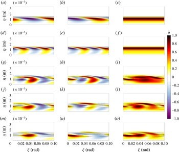
. Figure 12 shows disturbance contours at
 $x=0.34$
m and
 $F=30$
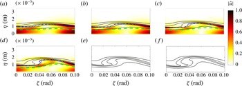
kHz for the various unstable modes along with a comparison with LST. The third row (g–i), fourth row (j–l) and fifth row (m–o) of panels correspond to modes 1, 2 and 3, respectively, from spatial BiGlobal theory. Then, the first column (g,j,m), second column (h,k,n) and third column (i,l,o) of panels for these rows show contours of the real part, the imaginary part and the magnitude, respectively, of the SBG eigenfunction
 $\hat{u} (\unicode[STIX]{x1D702},\unicode[STIX]{x1D701})$
.
For further consideration, the first row of panels (a–c) in figure 12 is included to show contours from LST applied to the undisturbed laminar basic state for travelling crossflow of wavenumber
 $m$
, while the second row of panels (d–f) shows contours from LST for travelling crossflow of wavenumber
 $2m$
. Then, the first column (a,d), second column (b,e) and third column (c,f) of panels for these rows show contours of the real part, the imaginary part and the magnitude, respectively, of
 $\hat{u} (\unicode[STIX]{x1D702})\exp (\text{i}m\unicode[STIX]{x1D701})$
or
 $\hat{u} (\unicode[STIX]{x1D702})\exp (2\text{i}m\unicode[STIX]{x1D701})$
(as appropriate) from LST.
Looking down the first column in figure 12, there are similar trends for all of modes 1, 2 and 3 and LST with concentrations in the boundary layer and near the wall. The same can be observed for the second column. This helps to verify that modes 1, 2 and 3 are variations of travelling crossflow. As discussed by Malik et al. (Reference Malik, Li and Chang1996), the interaction of strong stationary and travelling crossflow waves leads to multiple travelling crossflow modes. The progression of the SBG mode shapes for modes 1, 2 and 3 (at their respective peak frequencies) can then be seen in figures 13–15, respectively, for the axial locations
 $x=0.34{-}0.39$
m.
Isocontours of (a,d,g,j,m)
 $\hat{u} _{r}$
, (b,e,h,k,n)
 $\hat{u} _{i}$
and (c,f,i,l,o)
 $|\hat{u} |$
and five isolines of
 $\bar{\unicode[STIX]{x1D70C}}\bar{u}^{\ast }$
(black solid lines) for LST of unperturbed basic state with (a–c)
 $m$
and (d–f)
 $2m$
and for SBG of perturbed basic state with (g–i) mode 1, (j–l) mode 2 and (m–o) mode 3. The selected position is
 $x=0.34$
m and the frequency is
 $F=30$
kHz.

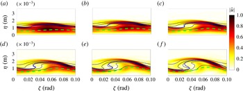
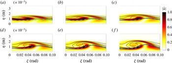
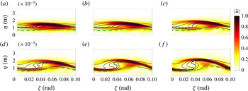
Based on the low frequencies of these unstable disturbances, as well as the mode shapes, it is clear that these are variations of travelling crossflow modes. Mode 1 and mode 2 have very similar disturbance concentrations and development. It is important to visualize that they appear as an instability near the wall upstream, but, as the wave grows in amplitude, the disturbance gets modulated until the concentration appears strongly in the trough and upwelling of the wave, similar to previous low-speed results (White & Saric Reference White and Saric2005).
Isocontours of
 $|\hat{u} |$
of mode 1, five isolines of
 $\bar{\unicode[STIX]{x1D70C}}\bar{u}^{\ast }$
(black solid lines), critical layer (blue dotted line) and relative sonic line (green dashed line) for (a)
 $x=0.34$
m, (b)
 $x=0.35$
m, (c)
 $x=0.36$
m, (d)
 $x=0.37$
m, (e)
 $x=0.38$
m and (f)
 $x=0.39$
m. The selected frequency is
 $F=45$
kHz.

Isocontours of
 $|\hat{u} |$
of mode 2, five isolines of
 $\bar{\unicode[STIX]{x1D70C}}\bar{u}^{\ast }$
(black solid lines), critical layer (blue dotted line) and relative sonic line (green dashed line) for (a)
 $x=0.34$
m, (b)
 $x=0.35$
m, (c)
 $x=0.36$
m, (d)
 $x=0.37$
m, (e)
 $x=0.38$
m and (f)
 $x=0.39$
m. The selected frequency is
 $F=55$
kHz.

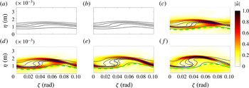
Also, mode 3 begins to develop as a result of the travelling crossflow modulation. This can be seen in figures 9 and 10, where it is clear that mode 3 does not exist upstream of
 $x=0.34$
m.
Isocontours of
 $|\hat{u} |$
of mode 3, five isolines of
 $\bar{\unicode[STIX]{x1D70C}}\bar{u}^{\ast }$
(black solid lines), critical layer (blue dotted line) and relative sonic line (green dashed line) for (a)
 $x=0.34$
m, (b)
 $x=0.35$
m, (c)
 $x=0.36$
m, (d)
 $x=0.37$
m, (e)
 $x=0.38$
m and (f)
 $x=0.39$
m. The selected frequency is
 $F=30$
kHz.

6.2.2 Type-I secondary instability
Using (4.1) at the most developed axial location of
 $x=0.39$
m, type-I secondary instabilities are predicted to appear at approximately
 $F=128$
kHz. Mode 2, peak 2 appears unstable in the range
 $F=70{-}155$
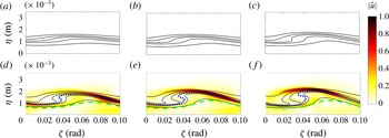
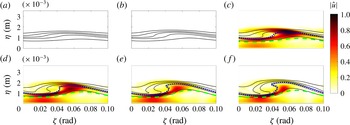
kHz, which includes that predicted frequency. Furthermore, the mode shape can be seen in figure 16. It is clear that, as the disturbance grows more unstable, and the nonlinearities become large, the concentration appears on the shoulder of the wave. Based on figure 8, mode 2, peak 2 is a type-I secondary instability associated with the
 $(\bar{\unicode[STIX]{x1D70C}}^{\ast }/r)(\unicode[STIX]{x2202}\bar{u}^{\ast }/\unicode[STIX]{x2202}\unicode[STIX]{x1D701})$
generalized gradient.
Isocontours of
 $|\hat{u} |$
of mode 2, peak 2, five isolines of
 $\bar{\unicode[STIX]{x1D70C}}\bar{u}^{\ast }$
(black solid lines), critical layer (blue dotted line) and relative sonic line (green dashed line) for (a)
 $x=0.34$
m, (b)
 $x=0.35$
m, (c)
 $x=0.36$
m, (d)
 $x=0.37$
m, (e)
 $x=0.38$
m and (f)
 $x=0.39$
m. The selected frequency is
 $F=120$
kHz.

6.2.3 Type-II secondary instability
As described before, the type-II secondary instability follows the
 $\bar{\unicode[STIX]{x1D70C}}^{\ast }(\unicode[STIX]{x2202}\bar{u}^{\ast }/\unicode[STIX]{x2202}\unicode[STIX]{x1D702})$
generalized gradient (figure 8
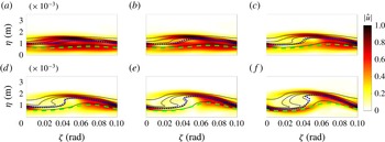
b). The easiest way to distinguish a type-II secondary instability is with the concentration of the disturbance on the crest of a stationary crossflow wave. The SBG mode shapes of modes 5 and 6 as seen in figures 17 and 18, respectively, clearly show the concentrations focused on the crest, and are type-II secondary instabilities. Furthermore, the growth rates from figure 10 show unstable type-II secondary instabilities in the range
 $F=140{-}300$
kHz, depending on the axial location. It is important to note that these frequencies are approximately double the frequencies of the type-I secondary instabilities and have a wider frequency band (White & Saric Reference White and Saric2005). Furthermore, these two modes seem to grow quickly and become the dominant disturbance feature by the saturation of the stationary crossflow, again consistent with the low-speed results.
Isocontours of
 $|\hat{u} |$
of mode 5, five isolines of
 $\bar{\unicode[STIX]{x1D70C}}\bar{u}^{\ast }$
(black solid lines), critical layer (blue dotted line) and relative sonic line (green dashed line) for (a)
 $x=0.34$
m, (b)
 $x=0.35$
m, (c)
 $x=0.36$
m, (d)
 $x=0.37$
m, (e)
 $x=0.38$
m and (f)
 $x=0.39$
m. The selected frequency is
 $F=165$
kHz.

Isocontours of
 $|\hat{u} |$
of mode 6, five isolines of
 $\bar{\unicode[STIX]{x1D70C}}\bar{u}^{\ast }$
(black solid lines), critical layer (blue dotted line) and relative sonic line (green dashed line) for (a)
 $x=0.34$
m, (b)
 $x=0.35$
m, (c)
 $x=0.36$
m, (d)
 $x=0.37$
m, (e)
 $x=0.38$
m and (f)
 $x=0.39$
m. The selected frequency is
 $F=200$
kHz.

6.2.4 Second mode instability
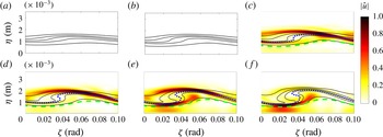
As mentioned earlier, the critical layer and relative sonic line help to distinguish a second mode instability from a secondary instability. Based on the concentrations in the amplitude functions, mode 4 (figures 19 and 20) seems to have second mode characteristics. As with the second mode, there is a concentration between the relative sonic line and the wall, with a second peak just above the critical layer. These second modes are unstable in the range
 $F=185{-}355$
kHz, depending on the axial location. Comparing with the LST second mode results in figure 10, the peak frequency is similar to the leftmost peak of mode 4. Furthermore, in figure 11 the LST second mode phase speeds are approximately the same as the leftmost peak at earlier axial locations. The disturbances associated with the leftmost peak are concentrated below the shoulder of the crossflow wave (figure 19), while the disturbances associated with the rightmost peak are concentrated in the trough (figure 20). As the concentration moves from the shoulder to the trough, the boundary layer shrinks and the frequency grows. This is another sign that mode 4 and mode 4, peak 2 are second modes. Finally, these do not appear to be harmonics of each other, as their concentrations in the boundary layer are different from one mode to the other.
Isocontours of
 $|\hat{u} |$
of mode 4, five isolines of
 $\bar{\unicode[STIX]{x1D70C}}\bar{u}^{\ast }$
(black solid lines), critical layer (blue dotted line) and relative sonic line (green dashed line) for (a)
 $x=0.34$
m, (b)
 $x=0.35$
m, (c)
 $x=0.36$
m, (d)
 $x=0.37$
m, (e)
 $x=0.38$
m and (f)
 $x=0.39$
m. The selected frequency is
 $F=235$
kHz.

Isocontours of
 $|\hat{u} |$
of mode 4, peak 2, five isolines of
 $\bar{\unicode[STIX]{x1D70C}}\bar{u}^{\ast }$
(black solid lines), critical layer (blue dotted line) and relative sonic line (green dashed line) for (a)
 $x=0.34$
m, (b)
 $x=0.35$
m, (c)
 $x=0.36$
m, (d)
 $x=0.37$
m, (e)
 $x=0.38$
m and (f)
 $x=0.39$
m. The selected frequency is
 $F=295$
kHz.

6.2.5 Coexisting instabilities
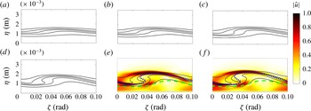
Finally, the primary and secondary instabilities seem to coexist. It is important to note there are no interactions among the instabilities, as the SBG analysis is linear, but they do both appear together at certain frequencies when both are unstable. In figures 21 and 22, for example, the second mode and the type-II secondary instability appear together over a frequency range. Following the evolution downstream, mode 5, peak 2 (figure 21) develops more concentration on the crest, favouring the type-II secondary instability at
 $F=205$
kHz, whereas mode 6, peak 2 (figure 22) develops more concentration closer to the wall and slightly above the critical layer, favouring the second mode at
 $F=290$
kHz. As the modified basic state becomes highly distorted (
 $x=0.39$
m), it is observed that, beyond a certain frequency, type-II secondary instabilities disappear, leaving the second mode to dominate.
Isocontours of
 $|\hat{u} |$
of mode 5, peak 2, five isolines of
 $\bar{\unicode[STIX]{x1D70C}}\bar{u}^{\ast }$
(black solid lines), critical layer (blue dotted line) and relative sonic line (green dashed line) for (a)
 $x=0.34$
m, (b)
 $x=0.35$
m, (c)
 $x=0.36$
m, (d)
 $x=0.37$
m, (e)
 $x=0.38$
m and (f)
 $x=0.39$
m. The selected frequency is
 $F=205$
kHz.

Isocontours of
 $|\hat{u} |$
of mode 6, peak 2, five isolines of
 $\bar{\unicode[STIX]{x1D70C}}\bar{u}^{\ast }$
(black solid lines), critical layer (blue dotted line) and relative sonic line (green dashed line) for (a)
 $x=0.34$
m, (b)
 $x=0.35$
m, (c)
 $x=0.36$
m, (d)
 $x=0.37$
m, (e)
 $x=0.38$
m and (f)
 $x=0.39$
m. The selected frequency is
 $F=290$
kHz.

6.3 Craig & Saric (Reference Craig and Saric2016) experimental comparison
Using hot-wire anemometry and mapping out the disturbances within the crossflow boundary layer, Craig & Saric (Reference Craig and Saric2016) focused their experiment below the hot-wire frequency response of 180 kHz. They filtered the data and found travelling crossflow within the range
 $F=15{-}60$
kHz and the secondary instability within the band
 $F=80{-}130$
kHz. These ranges coincide with the present mode 1, 2 and 3 for travelling crossflow and mode 2, peak 2 for the secondary instability. Looking at their band-passed contours, they noticed travelling crossflow concentrated in the trough and slightly up the shoulder, resembling mode 2 (figure 14). They saw the secondary instability disturbance concentrations on the shoulder (figure 8
a), resembling mode 2, peak 2 (figure 16). It is important to recall that the vortex path from the computational efforts intersects with the experimental measurement locations, and the crossflow amplitude and wavelength for secondary analysis compare well. The experiment and the computations agree that these modes are travelling crossflow and type-I secondary instabilities, respectively.
7 Ward et al. (Reference Ward, Henderson and Schneider2015) experimental conditions and comparison – artificial discrete roughness
7.1 Primary instability analysis
In a different experiment, Ward et al. (Reference Ward, Henderson and Schneider2015) measured multiple distinct frequency ranges at the wall with Kulite and PCB sensors, and provided data at an axial location of
 $x=0.36$
m and azimuthal angles of
 $\unicode[STIX]{x1D703}=115^{\circ },117.5^{\circ },120^{\circ },121^{\circ },122.5^{\circ }$
from windward. While the Craig & Saric (Reference Craig and Saric2016) polished model had a natural surface roughness distribution, Ward et al. (Reference Ward, Henderson and Schneider2015) added 50 evenly spaced discrete roughness elements (DREs) around the azimuth of the cone at
 $x=50.8$
mm for their experiment. This produces a large initial amplitude for the stationary crossflow disturbance with approximately
 $m=50$
after the
 $\unicode[STIX]{x1D703}$
–
 $\unicode[STIX]{x1D701}$
transformation; this will be the dominant disturbance evolving downstream. Based on the work of Oliviero et al. (Reference Oliviero, Kocian, Moyes and Reed2015), a vortex path that intersects the measurement location of
 $x=0.36$
m between
 $\unicode[STIX]{x1D703}=115^{\circ }$
and
 $122.5^{\circ }$
(figure 23
a) from the windward plane would lead to a local
 $\unicode[STIX]{x1D701}$
-direction wavenumber of approximately
 $m=14$
(figure 23
b) at
 $x=0.36$
m.
(a) Vortex path evolution of angle from windward plane; intersects
 $118^{\circ }$
at
 $0.36$
m. (b) The
 $\unicode[STIX]{x1D701}$
-direction-wavenumber (
 $m$
) variation at different axial locations; intersects
 $m=50$
at
 $x=0.0508$
m.

As the DRE heights are not known for the experiment, the present work assumed the DRE height from the DNS of Balakumar & Owens (Reference Balakumar and Owens2010) with its correlated
 $\hat{u} _{0,1}$
as the initial amplitude disturbance for EPIC (with the addition of the complex conjugate) to complete NPSE and SBG analyses. The
 $m=50$
(at
 $x=0.0508$
m) disturbance is then initialized at
 $x=0.1$
m with an initial amplitude (
 $\hat{u} _{0,1}$
) of
 $9.5\times 10^{-3}$
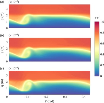
. From our NPSE analysis, this creates ‘flat-top’ developed mass flux crossflow vortices (modified basic states) that can be qualitatively verified in Balakumar & Owens (Reference Balakumar and Owens2010). Figure 24 shows the modified basic states at axial locations of
 $0.395$
,
 $0.40$
and
 $0.405$
m, and these will be discussed further.
Isocontours of modified basic state
 $x$
component of the mass flux,
 $\bar{\unicode[STIX]{x1D70C}}\bar{u}^{\ast }$
(3.4), at (a)
 $x=0.395$
m, (b)
 $x=0.40$
m and (c)
 $x=0.405$
m.

7.2 Secondary instability analysis
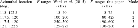
Focusing on the dominant peaks in their reported spectra, Ward et al. (Reference Ward, Henderson and Schneider2015) noted that: (1) for all of the azimuthal angles, there is a frequency band of
 $F=15{-}40$
kHz; (2) for
 $\unicode[STIX]{x1D703}=117.5^{\circ },120^{\circ }$
, there are two clear frequency bands of
 $F=100{-}200$
kHz and
 $F=250{-}500$
kHz; and (3) for
 $\unicode[STIX]{x1D703}=121^{\circ },122.5^{\circ }$
, there is a clear frequency band of
 $F=125{-}275$
kHz (see their figure 35). See table 3.
Comparison of Ward et al. (Reference Ward, Henderson and Schneider2015) observed frequencies (kHz) at indicated azimuthal locations and SBG calculated frequencies (kHz) with unstable growth rates over a crossflow wavelength and each designated mode number. The computational
 $\unicode[STIX]{x1D701}$
locations have been converted to
 $\unicode[STIX]{x1D703}$
locations for comparison.

These modified basic states shown are quite different from the Craig & Saric (Reference Craig and Saric2016) comparison modified basic states and produce different SBG results. SBG analysis at various axial locations from 0.36 to 0.39 m found only modulated travelling crossflow and a second mode. At
 $x=0.395$
m, the crossflow vortices are large enough to lead to secondary instabilities, and at
 $x=0.405$
m, the SBG results are consistent with the results of Ward et al. (Reference Ward, Henderson and Schneider2015). These results are not at the exact same axial location as the Ward et al. (Reference Ward, Henderson and Schneider2015) experiment, probably due to the uncertainty in the initial amplitude, but (1) stationary crossflow follows a vortex path and their azimuthal measurement locations include the vortex path in figure 23(a), (2) the
 $\unicode[STIX]{x1D701}$
-direction wavenumber changes by less than
 $1$
throughout the various axial locations, and (3) the axial locations are close to the experimental axial location. Therefore, SBG results of the modified basic states shown in figure 24 can offer a physical explanation of the results of the Ward et al. (Reference Ward, Henderson and Schneider2015) experiment.
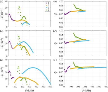
The SBG analysis of the modified basic states captures four distinct modes over a broad frequency band
 $F\in (0,600)$
kHz at axial locations of
 $0.395$
,
 $0.40$
and
 $0.405$
m, respectively, depicted in figure 25. The first column (a,c,e) shows the growth rates,
 $-\unicode[STIX]{x1D6FC}_{i}$
, of unstable modes and the second column (b,d,f) depicts the phase speeds,
 $c_{ph}$
. It appears that mode 1 and mode 4 have relatively constant growth rates between axial locations, mode 2 has relatively constant growth rates and a widening frequency band, and mode 3 has increasing growth rates at further downstream locations and its frequency band increases. Mode 2 and mode 3 are stable before
 $x=0.395$
m and they grow unstable quickly. Looking at the most developed case,
 $x=0.405$
m, mode 1 appears in the frequency range of
 $F\in (5,75)$
kHz; mode 2 appears in
 $F\in (80,425)$
kHz; mode 3 appears in
 $F\in (190,600)$
kHz; and mode 4 appears in
 $F\in (130,260)$
kHz. The SBG frequency bands of the modes with unstable growth rates predicted in total over a whole crossflow wavelength contain the Ward et al. (Reference Ward, Henderson and Schneider2015) frequency bands reported at individual azimuthal angles. See table 3.
Growth rate,
 $-\unicode[STIX]{x1D6FC}_{i}$
, of unstable modes at (a)
 $x=0.395$
m, (c)
 $x=0.40$
m and (e)
 $x=0.405$
m. Phase speed,
 $c_{ph}$
, of unstable modes at (b)
 $x=0.395$
m, (d)
 $x=0.40$
m and (f)
 $x=0.405$
m. Frequencies in the range
 $F\in (0,600)$
kHz.

When analysing these four modes, Ward et al. (Reference Ward, Henderson and Schneider2015) found that different frequency bands appear and vanish at different azimuthal angles. Looking at the modified basic states (figure 24) and converting
 $\unicode[STIX]{x1D701}$
to
 $\unicode[STIX]{x1D703}$
, the wavelength of a crossflow wave spans approximately
 $\unicode[STIX]{x1D703}=24^{\circ }$
around the azimuth, whereas their measurements were over
 $7.5^{\circ }$
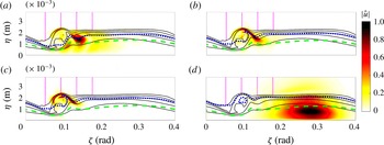
. Furthermore, looking at the mode shapes (figure 26) of each of the four modes at
 $x=0.405$
m, it is apparent that these modes produce disturbance concentrations in significantly different azimuthal angle regions. Referencing the four magenta vertical dotted lines (azimuthal angle locations from windward plane of
 $\unicode[STIX]{x1D703}=115^{\circ }:2.5^{\circ }:122.5^{\circ }$
, left to right, transformed to
 $\unicode[STIX]{x1D701}=114.96^{\circ }:2.53^{\circ }:122.55^{\circ }$
) in figure 26, mode 1 exists over the entire region
 $\unicode[STIX]{x1D703}=115^{\circ }{-}122.5^{\circ }$
with very minimal concentration at
 $\unicode[STIX]{x1D703}=115^{\circ }$
, mode 2 is concentrated and would be strong at measurement locations
 $\unicode[STIX]{x1D703}=117.5^{\circ },120^{\circ }$
, mode 3 is concentrated and would be strong at
 $\unicode[STIX]{x1D703}=117.5^{\circ },120^{\circ }$
, and mode 4 is concentrated near the wall and can be seen at the locations
 $\unicode[STIX]{x1D703}=121^{\circ },122.5^{\circ }$
.
Using the same analysis from the earlier results, it is clear that mode 1 is a modulation of travelling crossflow and concentrates strongly in the trough and slightly in the upwelling of the wave. Mode 2 is a type-I secondary instability that concentrates on the shoulder and mode 3 is a type-II secondary instability that concentrates on the crest of the stationary crossflow wave. Furthermore, mode 3 is approximately double the frequency of mode 2, which further confirms their secondary instability nature. Finally, mode 4 is clearly a second mode, which concentrates below the relative sonic line near the wall, and slightly above the critical layer.
Isocontours of
 $|\hat{u} |$
, five isolines of
 $\bar{\unicode[STIX]{x1D70C}}\bar{u}^{\ast }$
(black solid lines), critical layer (blue dotted line) and relative sonic line (green dashed line), and azimuthal angle locations from windward plane of
 $\unicode[STIX]{x1D703}=115^{\circ }:2.5^{\circ }:122.5^{\circ }$
(four magenta vertical dotted lines with increasing
 $\unicode[STIX]{x1D703}$
from left to right converted to
 $\unicode[STIX]{x1D701}=114.96^{\circ }:2.53^{\circ }:122.55^{\circ }$
) at
 $x=0.405$
m, for (a) mode 1 at
 $15$
kHz, (b) mode 2 at
 $125$
kHz, (c) mode 3 at
 $375$
kHz and (d) mode 4 at
 $140$
kHz.

Based on this analysis, Ward et al. (Reference Ward, Henderson and Schneider2015) are possibly measuring this modified basic state’s modulated travelling crossflow, secondary instabilities and second mode. Furthermore, these modes appear at certain azimuthal angles and vanish at others, as do the matching frequency bands from the experiment.
8 Incompressible swept wing comparison
Putting all the results together, the trends seem to be similar to those for an incompressible swept wing (White & Saric Reference White and Saric2005). There are multiple unstable modes over a large frequency spectrum. Travelling crossflow becomes modulated downstream significantly and does not appear as the same travelling crossflow in the linear regime. Type-I secondary instabilities remain unstable over a long axial distance and appear on the shoulder and their frequency is well predicted by (4.1). The higher-frequency type-II modes are on the crest and become unstable further downstream. Type-II instabilities appear to be approximately double the frequency of the type-I instability and their frequency bandwidth is larger. Once the secondary instabilities appear, they grow quickly and become dominant in the modified basic state. In the low-speed case, their appearance is a harbinger of breakdown to turbulence.
9 Conclusion
Coupling a nonlinear parabolized stability equation approach, with a methodology to predict the vortex path and the
 $\unicode[STIX]{x1D701}$
-direction-wavenumber evolution, and a spatial BiGlobal method approach, secondary instabilities of stationary crossflow at hypersonic speeds have been studied on a yawed straight circular cone, under the conditions of two quiet tunnel experiments, each with a different surface-roughness condition. The results demonstrate that upstream-induced number of waves around the azimuth (associated with the upstream surface-roughness condition) differ from expected values downstream and affect the modified basic state.
Under the natural roughness conditions of the Craig & Saric (Reference Craig and Saric2016) experiment, considering the resulting nonlinearly distorted basic state (due to the presence of the stationary crossflow) with low-momentum fluid over high-momentum fluid and the appearance of new inflection points in the downstream profiles, multiple instabilities are found, including travelling crossflow, secondary instabilities and second modes. The travelling crossflow begins concentrated near the wall and then, as it is more modulated by the stationary crossflow wave, it concentrates in the trough and upwelling of the wave. The secondary instabilities fall into two categories, type I and type II. Type I appears along the shoulder and type II appears on the crest. The second mode appears near the wall and extends through the boundary layer, with a concentration slightly above the critical layer as well. There is qualitative and quantitative agreement with the experimental results of Craig & Saric (Reference Craig and Saric2016), and it is agreed that the modes observed by Craig & Saric (Reference Craig and Saric2016) are travelling crossflow and the type-I secondary instability.
Under the DRE conditions of the Ward et al. (Reference Ward, Henderson and Schneider2015) experiment, a complete NPSE and SBG analysis was done. While we cannot conclude that the modified basic state NPSE achieved is exactly the same as the Ward et al. (Reference Ward, Henderson and Schneider2015) experiment, the SBG results offer a quantitative physical explanation of the experimental findings of Ward et al. (Reference Ward, Henderson and Schneider2015), in terms of frequency bands and why modes appear at certain azimuthal angles and vanish at others. The SBG results suggest that travelling crossflow, type-I and type-II secondary instability, and second mode frequencies are being measured in the Ward et al. (Reference Ward, Henderson and Schneider2015) experiment.
Finally, there are similarities between the secondary instabilities associated with the nonlinear evolution of both hypersonic and incompressible stationary crossflow.
Acknowledgements
This work is supported by Program Manager R. Ponnappan under AFOSR grant FA9550-14-1-0365. The authors are grateful to Pointwise for providing the gridding software, NASA for providing DPLR, and to Megan Heard and Lindsay Kirk for providing this basic state.