



1. Introduction
Introducing an external stochastic source to systems in fluid dynamics is now a common approach to study turbulence. Although turbulent flows are governed by the deterministic Navier–Stokes equations, their complex multiple-scale behaviours make them appear random for many practical purposes and it is therefore common to drive them using a stochastic forcing, very often Gaussian white noise in time. Theories of stochastic processes may in turn help to provide insights about the statistics of turbulence.
In many instances of natural phenomena and engineering, turbulence exists together with large-scale mean flows. Examples include zonal flows on Earth, Jupiter and in tokamak devices; see Galperin & Read (Reference Galperin and Read2019) for a comprehensive introduction. The interaction between turbulence and mean flows has thus become a key topic in fluid mechanics. While high-resolution numerical simulations can provide accurate solutions and comprehensive details, the alternative approach of establishing reduced models is also very useful: in particular, one can easily identify the essential physics from the equations and the computational cost is significantly reduced. Aligned with the latter approach, Farrell & Ioannou (Reference Farrell and Ioannou2003) built a compact model involving two equations to govern this process: one describes the turbulence modified by the mean flow, and the other describes the mean flow driven by the Reynolds stress of the turbulence. Using this model, they computed the profiles of zonal jets in a turbulent environment and analysed their stability. They referred to the stability theory as ‘stochastic structural stability theory’ (SSST), meaning the stability of jet profiles in stochastic waves. Tobias et al. (Reference Tobias, Dagon and Marston2011) established a similar system of turbulence–mean-flow interaction and successfully realised the spontaneous generation of jets on a rotating sphere. Using the same framework, Bakas & Ioannou (Reference Bakas and Ioannou2011) and Srinivasan & Young (Reference Srinivasan and Young2012) showed that the state of stochastic waves with zero mean flow can be linearly unstable, and weak zonal flows can grow exponentially to form strong zonal jets. This provides a new mechanism for zonal jet formation, and the instability has been termed ‘zonostrophic instability’ by Srinivasan & Young (Reference Srinivasan and Young2012). Building on these foundations, researchers have incorporated additional effects such as magnetic fields (Constantinou & Parker Reference Constantinou and Parker2018) and stratification (Fitzgerald & Farrell Reference Fitzgerald and Farrell2018), and Parker & Krommes (Reference Parker and Krommes2013, Reference Parker and Krommes2014) have extended the theory to weak nonlinearity, showing that the generation of jets can be understood in terms of the theory of pattern formation.
The theoretical framework of many of the studies cited above can be summarised abstractly in the following form:
 \begin{align} \frac {\mathrm{d}C}{\mathrm{d}t}+L(U,C)&=\varXi +D(C), \\[-12pt]\nonumber \end{align}
 \begin{align} \frac {\mathrm{d}U}{\mathrm{d}t}+R(C)&=D(U), \end{align}
where
 $C$
represents the correlation function(s) composed of the statistical average of the quadratic product of turbulent variables,
 $U$
is the zonal mean velocity,
 $L$
is a bilinear operator describing the linear evolution of waves in the mean flow,
 $\varXi$
represents the forcing,
 $R$
is a linear operator representing the effect of the Reynolds stress and
 $D$
is the linear operator for damping. For example, for two-dimensional flows described by a streamfunction
 $\psi$
via
 $(u,v)=(-\psi _{\!y},\psi _x)$
, we may decompose
 $\psi$
into
 \begin{equation} \psi (x,y,t)=\overline {\psi }(y,t)+\psi '(x,y,t),\quad \overline {\psi }=\frac {k}{2\pi }\int _0^{\frac {2\pi }{k}} \psi \,\mathrm{d}x, \end{equation}
where the overline represents the zonal average that is taken to be in the
 $x$
-direction with
 $k$
being the wavenumber of one periodic domain, and the prime denotes turbulence or waves. In the framework of Srinivasan & Young (Reference Srinivasan and Young2012), with vorticity
 $\zeta ={\nabla} ^2\psi$
, the correlation function and the zonal flow are
 \begin{equation} C(x_1,x_2,y_1,y_2,t)=\mathbb{E}[\zeta '(x_1, y_1,t)\,\zeta '(x_2,y_2,t)],\quad U=\frac {k}{2\pi }\int _0^{\frac {2\pi }{k}} u\,\mathrm{d}x, \end{equation}
where
 $\mathbb{E}$
denotes the expectation, statistical average or ensemble average of a sufficiently large number of stochastic realisations. The symbol
 $\varXi$
is the amplitude of the ensemble average of the forcing
 \begin{equation} \mathbb{E}[F(\boldsymbol{x}_1,t_1)\,F(\boldsymbol{x}_2,t_2)]=\delta (t_2-t_1)\varXi (x_1,x_2,y_1,y_2), \end{equation}
where
 $F$
is the forcing in the vorticity equation (cf. (2.1) introduced later). The
 $\delta$
-function results from the forcing
 $F$
having a stochastic Gaussian white noise dependence in time, which brings in stochasticity to the flow as a basic model of turbulence. One can identify the operators
 $L$
,
 $R$
and
 $D$
in (30), (31) and (34) of Srinivasan & Young (Reference Srinivasan and Young2012). Tobias et al. (Reference Tobias, Dagon and Marston2011) refer to the approach to derive systems like (1.1) and (1.2) as the ‘second-order cumulant expansion’ (CE2), as it incorporates statistical averages up to quadratic terms. They also refer to numerical simulations of these systems as ‘direct statistical simulation’ (DSS). A review of these statistical methods for turbulence is given in Marston & Tobias (Reference Marston and Tobias2023).
The system of (1.1) and (1.2) has furnished both computational and analytical progress in the analysis of wave–mean interaction. Tobias et al. (Reference Tobias, Dagon and Marston2011) have shown that simulations based on this system require far less computational resource than the original fluid equations, and moreover, directly provide the statistics of turbulence. Farrell & Ioannou (Reference Farrell and Ioannou2003) have found fixed points in this system and analysed their stability, corresponding to the stability of jet profiles in turbulent flows. Bakas & Ioannou (Reference Bakas and Ioannou2011) and Srinivasan & Young (Reference Srinivasan and Young2012) considered the stability of fixed points with
 $U=0$
, accounting for zonostrophic instability. Remarkably, Srinivasan & Young (Reference Srinivasan and Young2012) derived a compact dispersion relation that determines the growth rate, providing deep insights to the underlying physics of jet formation.
The construction of (1.1) and (1.2) requires two key assumptions. The first assumption is the ‘quasi-linear approximation’. It argues that we only need to retain nonlinearity involving mean flows as in
 $L(U,C)$
, where the wave–wave interaction or eddy–eddy interaction has been neglected. The second assumption is the ‘ergodic assumption’. It is that the zonal mean of any flow variable
 $a$
is equivalent to its ensemble mean
 \begin{equation} \overline {a}=\mathbb{E}[a]. \end{equation}
A direct consequence of the ergodic assumption is that the zonal mean flow
 $U=\mathbb{E}[u]$
, i.e. it is no longer stochastic. This will be the main issue that we examine in this paper.
Both the quasi-linear approximation and the ergodic assumption are widely used, but their validity remains an active topic of research. Here, we focus on the second one: the ergodic assumption. The concept that the zonal mean equals the ensemble mean is physically intuitive and may have links to theories of turbulence and stochastic processes. The ergodic assumption is needed to establish the model of (1.1) and (1.2) because, in (1.1),
 $U$
needs to be deterministic to be consistent with the deterministic nature of
 $C$
and
 $\varXi$
, and, in (1.2),
 $U$
needs to be driven by the Reynolds stress which takes the zonal average, thus the ensemble mean in
 $C$
(cf. (1.4a
)) needs to be equivalent to the zonal mean.
A more careful look at the ergodic assumption, however, raises concerns regarding its validity. The original meaning of ergodicity is a stochastic process experiencing all possible states. In the context of zonal flows, it means that, in the zonal direction, all possible states in various realisations are present, and thus the zonal mean is equal to the ensemble mean. But this is not true in a quasi-linear system like (1.1) and (1.2), because without wave–wave interactions, the wavenumbers of the flow remain very limited. The spatial structure of the flow may be too simple to realise the complicated behaviours in various stochastic realisations. Two consequences of the ergodic assumption are that the zonal mean of any quantity is deterministic and that the ensemble mean is zonally homogeneous, but numerical simulations suggest that these do not hold in general. For example, Farrell & Ioannou (Reference Farrell and Ioannou2003) have shown that the ensemble average of the zonal mean flow from a finite number of stochastic simulations is different than the average over infinitely many simulations predicted by the SSST theory, hence the zonal mean flow is stochastic. Simonnet et al. (Reference Simonnet, Rolland and Bouchet2021) further revealed that such stochasticity can randomly switch jet configuration, in particular changing the number of jets. Also, Bakas & Ioannou (Reference Bakas and Ioannou2013, Reference Bakas and Ioannou2014) have shown that in the ensemble mean of a flow field, non-zonal coherent structures can emerge through instability in a similar manner as zonostrophic instability forms zonal jets. These observations cast strong doubts on the validity of the ergodic assumption.
The issue of the ergodic assumption is exposed more explicitly in generalised theories of CE2. As has been noted by Tobias et al. (Reference Tobias, Dagon and Marston2011), Tobias & Marston (Reference Tobias and Marston2017) and Marston et al. (Reference Marston, Qi and Tobias2019), the framework of CE2 actually allows various kinds of averages. While the zonal average for zonal flows is physically intuitive and easy to implement, it is also possible to use the ensemble average: for example, we may use
 $\mathbb{E}(u)$
in the place of
 $U$
in (1.1) and (1.2). Allawala et al. (Reference Allawala, Tobias and Marston2020) performed DSS based on CE2 using both the zonal and the ensemble average. They found that the two methods produce qualitatively similar but quantitatively different results, and the ensemble average agrees better with direct numerical simulations. The difference between the results of zonal and ensemble averages can be significant in general, raising more concerns about the application of the ergodic assumption. Theoretically, the ergodic assumption may be justified if the time scale of the mean flow is much longer than that of the waves, as in the study of Bouchet et al. (Reference Bouchet, Nardini and Tangarife2013), which takes the limit of weak forcing and weak dissipation, or if there is a scale separation between the waves and the zonal flow (Durston & Gilbert Reference Durston and Gilbert2016). However, these prescriptions are too restrictive compared with its wide application.
In view of the wide application of the ergodic assumption as well as its potential issues, a rigorous examination of its validity becomes necessary. In this paper, we will look at one consequence of the ergodic assumption: that the zonal mean flow is non-stochastic. We will examine the actual stochasticity of the zonal mean flow and its consequences using a simple canonical model of hydrodynamic zonostrophic instability, which allows for analytical insights. Through large numbers of stochastic simulations, we will demonstrate that zonal flows indeed exhibit considerable stochasticity in most cases, calling into question the applicability of the ergodic assumption.
A more important problem that we explore is the impact of this stochasticity on zonostrophic instability. If the stochasticity of the zonal mean flow is significant, how does this stochasticity modify the instability? The model of (1.1) and (1.2) cannot address this problem, because information on the mean-flow stochasticity is no longer present. We will adopt an alternative method to study zonostrophic instability, following our previous work (Wang et al. Reference Wang, Mason and Gilbert2024). The essence of this method is that we retain the stochasticity of the flow and study the evolution of weak mean flows in stochastic waves. Our analysis has shown that when the zonal mean flow is stochastic, it is its expectation or ensemble mean that grows exponentially, i.e. to study the stability of the state with
 $U=0$
we should set a normal mode form for the expectation of
 $U$
 \begin{equation} \mathbb{E}[U]=U_0\, e^{\mathrm{i}my+st}+\mathrm{c.c.}, \end{equation}
where
 $\mathrm{c.c.}$
denotes the complex conjugate,
 $U_0$
is a constant,
 $m$
is the cross-stream wavenumber and
 $s$
is the growth rate. Our analysis further showed that in order to obtain the dispersion relation between
 $m$
and
 $s$
, the actual assumption that we need to make is that the mean flow and the stochastic waves are statistically decorrelated so that
 \begin{equation} \mathbb{E}[\textit{UC}]=\mathbb{E}[U]\, \mathbb{E}[C] \end{equation}
for the variables in (1.1) and (1.2). We note that (1.8) is weaker than assuming that
 $U$
is non-stochastic,
 $U = \mathbb{E}[U]$
, as results from the ergodic assumption. The assumption (1.8) thus becomes the central topic of our study. It will not be true in general, and we will derive an expression for the correlation
 $\mathbb{E}[\textit{UC}]-\mathbb{E}[U]\, \mathbb{E}[C]$
when it is weak. It will allow us to identify when (1.8) is a good approximation so that the resulting dispersion relation is accurate. We can further take into account this correlation in the analysis and derive an improved dispersion relation which predicts more accurate growth rates. Finally, we will perform numerical simulations to assess the predictions of the theories against the quasi-linear and fully nonlinear systems.
The structure of the paper is as follows: in § 2, we present the theory of zonostrophic instability using a simple model, from which we introduce the wave–mean decorrelation assumption. We then study the stochasticity of zonal flows in § 3. There we will demonstrate the stochasticity of zonal mean flows, analyse the actual wave–mean correlation and study its effect on the instability growth rate. Concluding remarks are given in § 4.
2. The theory of zonostrophic instability
In this section, we outline the theory of zonostrophic instability, accounting for the spontaneous generation of mean flows in a field of stochastic waves, and follow the framework of our previous study (Wang et al. Reference Wang, Mason and Gilbert2024). We introduce the model in § 2.1, and then the theoretical analysis in § 2.2, paying particular attention to the assumptions made about the stochasticity of the mean flow.
2.1. The model
We consider a basic, non-dimensional model of two-dimensional flow on a
 $\beta$
-plane, governed by
 \begin{equation} \zeta _t-\psi _{\!y}\zeta _x+\psi _x\zeta _{\!y}+\beta \psi _x=F-\mu \zeta +\nu {\nabla} ^2 \zeta ,\quad \zeta ={\nabla} ^2\psi \,, \end{equation}
where
 $\psi$
is the streamfunction, the velocity is
 $(u,v)=(-\psi _{\!y},\psi _x)$
,
 $\zeta$
is the vorticity,
 $\beta$
is the gradient of the Coriolis parameter,
 $F$
is a prescribed external forcing,
 $\mu$
is a drag coefficient and
 $\nu$
is the viscosity. The forcing
 $F$
is stochastic to mimic a turbulent environment. We consider the simple forcing
 \begin{equation} F=\sigma \hat {\xi }(t)e ^{\mathrm{i}kx}+\mathrm{c.c.}, \end{equation}
where
 $\sigma$
is the forcing strength,
 $k$
is a zonal wavenumber and
 $\hat {\xi }$
is a complex stochastic white noise. It is specified and normalised according to
 \begin{equation} \mathbb{E}\bigl [\hat {\xi }(t)\, \hat {\xi }^*(\tau )\bigr ]=\delta (t-\tau ), \quad \mathbb{E}\bigl [\hat {\xi }(t)\, \hat {\xi }(\tau )\bigr ]=0,\quad \mathbb{E}\bigl [\hat {\xi }(t)\bigr ]=0. \end{equation}
For modelling most aspects of turbulence, (2.2) is too simple in spatial structure, with one single wavevector; nevertheless, it has been used in the fundamental work of Farrell & Ioannou (Reference Farrell and Ioannou2003) to build a basic model for turbulence–mean-flow interaction. In the present paper, this forcing is quite sufficient for us to determine key aspects of the stochasticity of the mean flow; more realistic forcings will be considered in future research.
Since the forcing is
 $y$
-independent, (2.1) has a solution with vanishing nonlinearity, namely
 \begin{equation} \psi = \psi _1=\hat {\psi }_1(t)e^{\mathrm{i}kx}+\mathrm{c.c.}, \end{equation}
with
 \begin{equation} \hat {\psi }_1=-\frac {\sigma }{k^2}\, e^{\lambda _1 t}\int ^t\hat {\xi }(\tau ) e^{-\lambda _1\tau }\mathrm{d}\tau ,\quad \lambda _1=-\mu -\nu k^2+\mathrm{i}\, \frac {\beta }{k}\, . \end{equation}
The zonal mean flow is defined as the spatial average of the streamwise velocity
 \begin{equation} U(y,t) =\overline {u}(y,t) \equiv \frac {k}{2\pi }\int _0^{2\pi /k}u(x,y,t)\,\mathrm{d}x, \end{equation}
and the solution (2.4) has
 $U=0$
. This solution thus describes a stochastic forced Rossby wave, with zero zonal mean flow, whose statistical properties follow from those of the white noise. For example, for
 $t\gt \tau$
,
 \begin{equation} \mathbb{E}\bigl [\hat {\psi }_1(\tau )\,\hat {\psi }_1^*(t)\bigr ]=-\frac {\sigma ^2}{k^4}\frac {1}{\lambda _1+\lambda _1^*} \, e^{\lambda _1^*(t-\tau )},\quad \mathbb{E}\bigl [\hat {\psi }_1(\tau )\,\hat {\psi }_1(t)\bigr ]=0,\quad \mathbb{E}\bigl [\hat {\psi }_1(t)\bigr ]=0, \end{equation}
indicating exponential decay of correlation with time difference
 $ t - \tau$
.
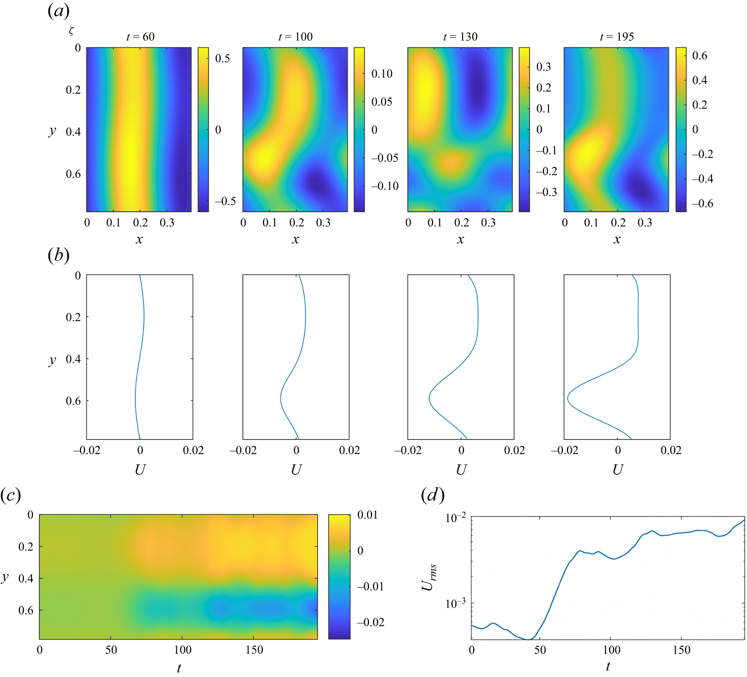
The state described by (2.4) can be unstable to zonostrophic instability: weak disturbances with mean zonal components can grow exponentially to form strong zonal jets. In figure 1, we show a numerical solution of (2.1) as an example. We use the initial condition
 $\psi =\varepsilon \cos my$
, with
 $\varepsilon =10^{-4}$
,
 $m=8$
at
 $t=0$
, which introduces a small disturbance to the state (2.4), of a weak mean flow
 $U=\varepsilon m\sin my$
. We solve the equations in a periodic domain using spectral methods, as in Wang et al. (Reference Wang, Mason and Gilbert2024). In panels
 $(a)$
and
 $(b)$
, we plot snapshots of the vorticity and mean-flow profiles. We see that the mean flow grows stronger and the vorticity field becomes more sinuous. Vortices and nonlinear patterns emerge at later times. In panel
 $(c)$
, we show the mean flow
 $U$
in
 $(y,t)$
space, as a Hovmöller diagram, and clearly observe the formation of two zonal jets in opposite directions. In panel
 $(d)$
, we plot the evolution of the root mean square (r.m.s.) of
 $U$
, averaged over the
 $y$
-direction and denoted
 $U_{\textit{rms}}(t)$
 \begin{equation} U_{\textit{rms}}= \biggl ( {\frac {m}{2\pi }\int _0^{{2\pi }/{m}}U^2\,\mathrm{d}y} \biggr )^{1/2}. \end{equation}
The value of
 $U_{\textit{rms}}$
shows quite an irregular dependence on time, but clearly grows and saturates, showing a period of rapid exponential growth between
 $t=40$
and
 $t=70$
, a manifestation of zonostrophic instability.
A numerical solution of equation (2.1) with initial condition
 $\psi =\varepsilon \cos my$
at
 $t=0$
and parameters
 $\beta =5$
,
 $\nu =10^{-4}$
,
 $\mu =0.01$
,
 $\sigma =0.05$
,
 $k=16$
,
 $m=8$
,
 $\varepsilon =10^{-4}$
. Depicted are
 $(a)$
the vorticity field
 $\zeta (x,y,t)$
and
 $(b)$
the mean profile
 $U(y,t)$
, at various times
 $t$
, together with
 $(c)$
plots of
 $U(t,y)$
and
 $(d)$
 $U_{\textit{rms}}(t)$
.

Figure 1. Long description
The image contains four panels labeled (a) through (d), each depicting different aspects of the interaction between turbulence and mean flows. Panel A shows four heat maps of vorticity fields at different times (t = 60, 100, 130, 195). The x-axis represents the horizontal position (x), and the y-axis represents the vertical position (y). The color scale indicates the vorticity values, ranging from -0.5 to 0.6. Panel B consists of four line graphs showing the mean profile (U) at the same times as Panel A. The x-axis represents the mean profile values, and the y-axis represents the vertical position (y). Panel C is a heat map showing the evolution of the mean profile (U) over time (t). The x-axis represents time, and the y-axis represents the vertical position (y). The color scale indicates the mean profile values, ranging from -0.02 to 0.01. Panel D is a line graph showing the root mean square (RMS) of the mean profile (U_rms) over time (t). The x-axis represents time, and the y-axis represents the RMS values. The graph shows an increasing trend in U_rms over time.
2.2. The theory
We now outline the theory of zonostrophic instability, explaining the flow transition described in § 2.1. We decompose the flow variables into a wave component denoted by a prime, and a zonal mean component denoted by a bar (cf. (2.6))
 \begin{equation} \psi =\overline {\psi }(y,t)+\psi '(x,y,t),\quad \zeta =\overline {\zeta }(y,t)+\zeta '(x,y,t)\,. \end{equation}
For analytical insight, we employ the quasi-linear approximation, neglecting the nonlinear interaction between waves except where it drives a mean flow, to give the following wave–mean-flow system:
 \begin{equation} \zeta '_t+U\zeta '_x+(\beta -U_{yy})\psi _x'=F-\mu \zeta '+\nu {\nabla} ^2\zeta ',\quad \zeta '={\nabla} ^2\psi ', \end{equation}
 \begin{equation} U_t-\left (\overline {\psi '_x\psi '_{\!y}}\right )_{\!y}=-\mu U+\nu U_{yy}. \end{equation}
It is quite sufficient to adopt the quasi-linear approximation for the goal of this paper, to investigate mean-flow stochasticity, and we expect our results to be valid for more complex models. Thus we adopt this approximation in the present paper without further examination of its validity or range of usefulness, where there remain open questions (see, e.g. Saxton et al. Reference Saxton, Marston, Oishi and Tobias2024).
The system (2.10) and (2.11) is stochastic in light of the stochasticity of
 $F$
. In order to examine the stochasticity of the mean flow, we first proceed without any ensemble averaging, but will take the expectation
 $\mathbb{E}$
of quantities later. At this point the above system is obtained with the bar denoting the spatial average or projection given in (2.6) and only the quasi-linear approximation has been applied; we stress that no statistical average has yet been taken.
Given the above basic state of
 $\psi _1$
in (2.4), (2.5) and
 $U=0$
, we now incorporate small disturbances including a possible zonal flow, writing
 \begin{equation} \psi '=\psi _1+\psi _2 + \ldots , \quad U=0+U_2 + \ldots . \end{equation}
We linearise equations (2.10) and (2.11) for
 $\psi _2$
and
 $U_2$
and then consider their Fourier components
 \begin{equation} U_2=\hat {U}(t) e^{\mathrm{i}my}+\mathrm{c.c.}, \quad \psi _2=\hat {\psi }_{2+}(t) e^{\mathrm{i}kx+\mathrm{i}my}+\hat {\psi }_{2-}(t) e^{-\mathrm{i}kx+\mathrm{i}my}+\mathrm{c.c.}, \end{equation}
to obtain an equation for the amplitude
 $\hat {U}$
(which for convenience we will also call the mean flow from now on)
 \begin{align} &\frac {\mathrm{d}\hat {U}}{\mathrm{d}t}+(\mu +\nu m^2)\hat {U} \nonumber \\ &=m^2k^2\varLambda \int ^t\hat {U}(\tau )\left [\hat {\psi }_1(\tau )\,\hat {\psi }_1^*(t) e^{-\lambda _2(\tau -t)}+\hat {\psi }_1^*(\tau )\,\hat {\psi }_1(t)e^{-\lambda _2^*(\tau -t)}\right ]\mathrm{d}\tau , \end{align}
where
 \begin{equation} \lambda _2=-\mu -\nu (k^2+m^2)+\frac {\mathrm{i}k\beta }{k^2+m^2}\, ,\quad \varLambda = \frac {k^2-m^2}{k^2+m^2}\, . \end{equation}
At this point, we stress that (after the application of the quasilinear approximation) the system given by (2.5) and (2.14) is exact and applies for any time dependence specified in
 $\hat \xi (t)$
; we have not made use of (2.3) or equivalently (2.7). However, if we now take expectations of the (2.14) to probe the behaviour of
 $\mathbb{E}[\hat U]$
we run into a closure problem: the evolution of
 $\mathbb{E}[\hat {U}]$
involves triple correlations such as
 $\mathbb{E}[\hat {U}(\tau ) \hat {\psi }_1(\tau ) \hat {\psi }_1^*(t)]$
.
A further assumption or approximation is then needed to make analytical progress. The assumption that authors typically make is the non-stochasticity of
 $\hat {U}$
following the ergodic assumption, as in the theories of SSST, DSS and CE2. We term this assumption the deterministic mean-flow assumption, or the deterministic assumption for short, mathematically written as
 \begin{equation} \hat {U} = \mathbb{E}\bigl [\hat {U} \bigr] \quad \text{(deterministic assumption)}, \end{equation}
in which case the triple correlations turn into double correlations which are known from (2.7). Alternatively, as shown in Wang et al. (Reference Wang, Mason and Gilbert2024), we can apply a weaker assumption which allows
 $\hat {U}$
to be random but takes its expectation to be separable from expectations of
 $\hat {\psi }_1$
. We term this assumption the wave–mean decorrelation assumption or the decorrelation assumption
 \begin{align} & \mathbb{E}\bigr [\hat {U}(\tau )\,\hat {\psi }_1(\tau )\,\hat {\psi }_1^*(t)\bigr ]=\mathbb{E}\bigl [\hat {U}(\tau ) \bigr] \, \mathbb{E}\bigl [\hat {\psi }_1(\tau )\,\hat {\psi }_1^*(t)\bigr ],\nonumber \\ & \mathbb{E}\bigr [\hat {U}(\tau )\,\hat {\psi }_1^*(\tau )\,\hat {\psi }_1(t)\bigr ]=\mathbb{E}\bigl [\hat {U}(\tau )\bigr ] \, \mathbb{E}\bigl [\hat {\psi }^*_1(\tau )\,\hat {\psi }_1(t)\bigr ]\quad \text{(decorrelation assumption)}. \end{align}
Note that (2.16) and (2.17) are termed as the full and partial ergodic assumptions in our earlier paper (Wang et al. Reference Wang, Mason and Gilbert2024). Both assumptions are closures, which will not be true in general but may either operate as good approximations in some regime, or may lead to predictions that are only qualitatively correct but are informative regarding the underlying physics (this being in common with the use of the quasi-linear approximation). Both give the same growth rate, but of
 $\hat {U}$
and
 $\mathbb{E}[\hat {U}]$
, respectively.
We apply the decorrelation assumption to the expectation of (2.14), which becomes
 \begin{align} &\frac {\mathrm{d}}{\mathrm{d}t}\, \mathbb{E}\bigl [\hat {U}(t) \bigr]+(\mu +\nu m^2)\,\mathbb{E}\bigl [\hat {U}(t) \bigr] \nonumber \\ &=m^2k^2\varLambda \int ^t\mathbb{E}\bigl [\hat {U}(\tau ) \bigr]\left \{\mathbb{E}\bigl [\hat {\psi }_1(\tau )\,\hat {\psi }_1^*(t) \bigr] e^{-\lambda _2(\tau -t)}+\mathbb{E}\bigl [\hat {\psi }_1^*(\tau )\,\hat {\psi }_1(t) \bigr]e^{-\lambda _2^*(\tau -t)}\right \}\mathrm{d}\tau ,\end{align}
and consider exponential growth of the mean flow, of the form
 \begin{equation} \mathbb{E}\bigl [\hat {U}(t) \bigr]=U_0\,e^{\textit{st}}. \end{equation}
Using (2.7a
) for the quadratic expectations in (2.18), we derive a dispersion relation for the growth rate
 $s$
 \begin{equation} s+\mu +\nu m^2=\frac {m^2\sigma ^2\varLambda }{2k^2(\mu +\nu k^2)}\left (\frac {1}{s-\lambda _1^*-\lambda _2}+\frac {1}{s-\lambda _1-\lambda _2^*}\right )\!. \end{equation}
We found that the solution of
 $s$
from this dispersion relation is always real, although we cannot show this analytically. We note that in other settings, complex values of
 $s$
representing vacillation of zonal mean flows can appear, for example, for non-zero basic flow profiles (Farrell & Ioannou Reference Farrell and Ioannou2003) or more complicated forcing structures (Ruiz et al. Reference Ruiz, Parker, Shi and Dodin2016). When
 $s$
is positive, the expectation of the zonal mean flow will grow exponentially, which explains what we see in figure 1
 $(d)$
. We will defer the detailed results from (2.20) and comparison with numerical simulations to § 4, after we discuss an improved theory.
The dispersion relation (2.20) may also be derived within the theoretical framework of Srinivasan & Young (Reference Srinivasan and Young2012) (see Appendix B of Wang et al. (Reference Wang, Mason and Gilbert2024)) and so our calculations lead to the same results as the theories of SSST or CE2. However, our approach is to use the decorrelation assumption (2.17), that the waves and the mean flow are statistically decorrelated, which is weaker than the deterministic assumption (2.16). Moreover, (2.14) has retained the stochasticity of the zonal mean flow, which allows us to investigate the two assumptions for the rest of the paper.
3. Stochasticity of zonostrophic instability
In this section, we study the stochasticity of zonostrophic instability. We first demonstrate the existence of stochasticity within the mean flow in § 3.1, contrary to the deterministic mean-flow assumption (2.16). Then, in § 3.2, we examine the wave–mean decorrelation assumption (2.17) through an approximate expression for the actual wave–mean correlation. Based on this result, we study the impact of the correlation on the dispersion relation in § 3.3.
3.1. Stochasticity of zonal mean flows
To investigate these assumptions and mean-flow stochasticity we return to the quasi-linear system (2.10, 2.11) with linearised disturbances (2.12, 2.13) before any ensemble averaging is applied. It is inconvenient to solve the resulting integro-differential equation (2.14) numerically, and so we resort to the equivalent low-order set of stochastic ordinary differential equations (ODEs) (cf. §§ 2.2, 2.3 of Wang et al. (Reference Wang, Mason and Gilbert2024))
 \begin{align} & \frac {\mathrm{d}\hat {\psi }_1}{\mathrm{d}t}-\lambda _1\hat {\psi _1} =-\frac {\sigma }{k^2}\, \hat {\xi }, \\[-12pt]\nonumber \end{align}
 \begin{align} & \frac {\mathrm{d}\hat {\psi }_{2+}}{\mathrm{d} t}-\lambda _2\hat {\psi }_{2+} =-\mathrm{i}k \varLambda \hat {U}\hat {\psi }_1, \\[-12pt]\nonumber \end{align}
 \begin{align} & \frac {\mathrm{d}\hat {\psi }_{2-}}{\mathrm{d} t}-\lambda _2^*\hat {\psi }_{2-} =\mathrm{i}k \varLambda \hat {U}\hat {\psi }_1^*, \\[-12pt]\nonumber \end{align}
 \begin{align} & \frac {\mathrm{d}\hat {U}}{\mathrm{d}t}+(\mu +m^2\nu )\hat {U} =\mathrm{i}m^2k(\hat {\psi }_{2+}\hat {\psi }_1^*-\hat {\psi }_{2-}\hat {\psi }_1). \end{align}
The initial condition is the same as that used for the simulations in figure 1. We solve this system with Itô’s interpretation and Euler’s method with a small time step of
 $\Delta t=10^{-3}$
. One may apply higher-order numerical schemes such as Runge–Kutta methods (e.g. Srinivasan & Young Reference Srinivasan and Young2012), but given the lack of smoothness of the white noise, it is not clear that higher-order schemes can provide much better performance.
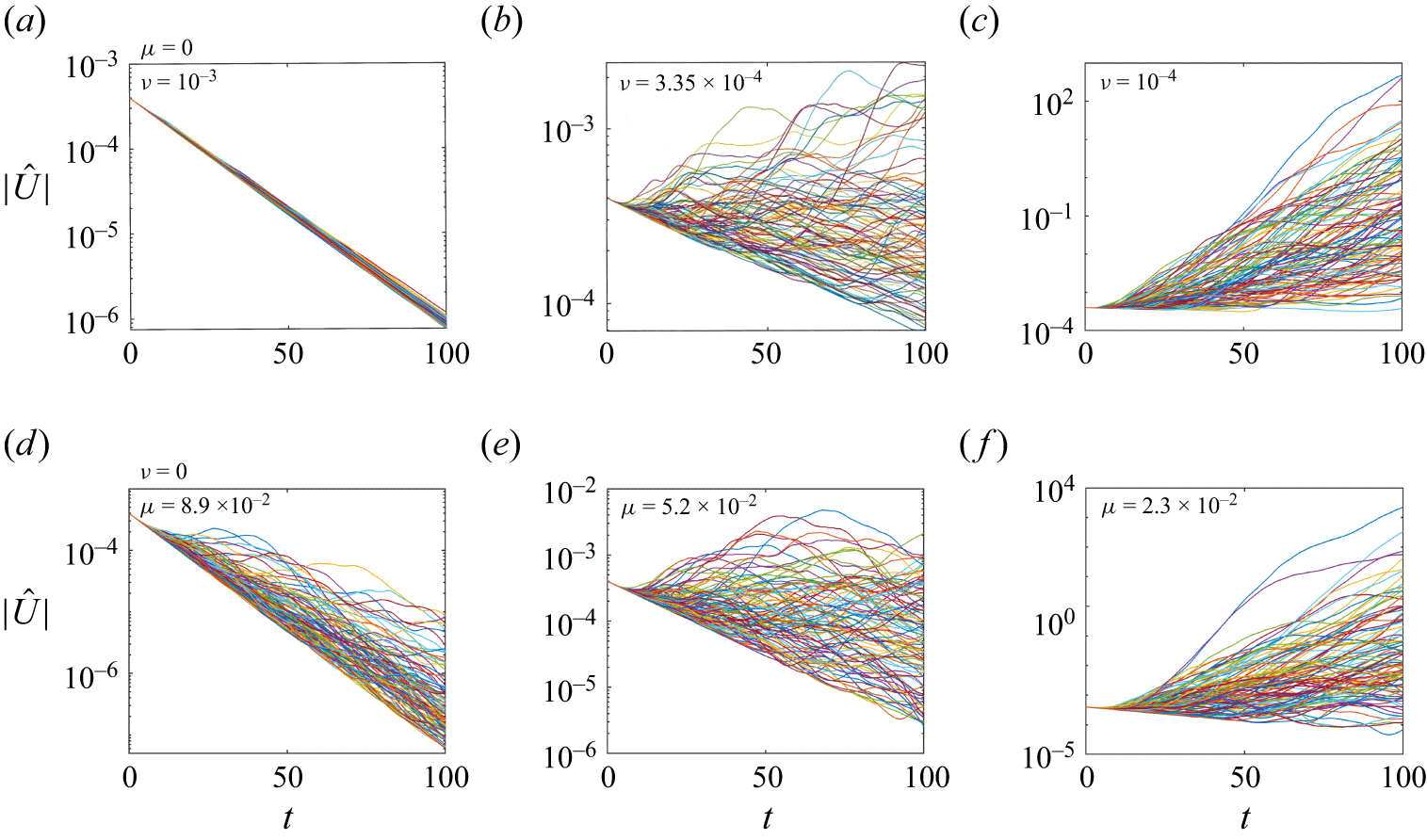
Numerical solutions of (3.1)–(3.4) are shown in figure 2. We undertake 100 realisations of the white noise in the forcing
 $F$
for each set of parameter values. Panels
 $(a$
–
 $c)$
show the results at various viscosities with zero drag coefficient, and panels
 $(d$
–
 $f)$
show the results at various drag coefficients with zero viscosity. We have chosen the parameters so that the growth rates predicted by (2.20) are the same for the two rows (see caption). In panel
 $(a)$
, where a relatively strong viscosity
 $\nu =10^{-3}$
suppresses zonostrophic instability, we see that
 $|\hat {U}|$
decays in all realisations in a similar manner. We conclude that the stochasticity of the zonal mean flow is indeed negligible in this case. However, when viscosity is reduced to
 $\nu =3.35\times 10^{-4}$
in panel
 $(b)$
, significant variation between different realisations emerges. We observe that
 $|\hat {U}|$
decays in some realisations but grows in others. In individual realisations,
 $|\hat {U}|$
also switches frequently between growth and decay, exhibiting considerable stochasticity. When viscosity is further reduced to
 $\nu =10^{-4}$
in panel
 $(c)$
, nearly all realisations demonstrate
 $|\hat {U}|$
growing exponentially, but the growth varies significantly: some grow to huge values, some reach a plateau after prominent growth, and some do not grow until very late on. Panels
 $(d$
–
 $f)$
, where the viscosity is zero and the drag coefficient increases, exhibit a similar pattern, demonstrating considerable stochasticity. We notice that curves of
 $|\hat {U}|$
in panels
 $(d$
–
 $f)$
show a much wider spread compared with panels
 $(a$
–
 $c)$
. Panel
 $(d)$
is especially remarkable: strong stochasticity is present even when
 $|\hat {U}|$
decays. Overall, the drag in panels
 $(d$
–
 $f)$
seems to allow rather stronger stochasticity in the mean flow, compared with viscosity in panels
 $(a$
–
 $c)$
, for the same theoretical growth rates.
Numerical solutions of equations (3.1)–(3.4) at
 $\beta =5$
,
 $\sigma =0.05$
,
 $k=16$
,
 $m=8$
. Panels
 $(a$
–
 $c)$
show the results at various viscosities with
 $\mu =0$
, and panels
 $(d$
–
 $f)$
show the results at various drag coefficients with
 $\nu =0$
. Each figure contains 100 realisations. The exponential growth rates of zonostrophic instability predicted by the dispersion relation (2.20) are
 $(a)$
,
 $(d)$
 $s=-0.061$
,
 $(b)$
,
 $(e)$
 $s=-9\times 10^{-4}$
,
 $(c)$
,
 $(f)$
 $s=0.081$
.

Through figure 2, we have demonstrated that in general, zonal mean flows exhibit considerable stochasticity, and the deterministic assumption (2.16) does not hold. Only when viscosity is strong can we confidently apply this assumption. This raises the question of what role this mean-flow stochasticity plays in the theory of zonostrophic instability, which we will explore in the next section.
3.2. The wave–mean correlation
As the deterministic assumption (2.16) is clearly poor in many contexts, next we turn to discussing the weaker decorrelation assumption (2.17), that the waves and the mean flow are statistically decorrelated. As this is certainly not an exact result in general, we will derive results based on the correlation being small rather than zero.
Equation (2.14) retains the stochasticity of the mean flow and can be exploited to compute the correlations. To do this, we convert it into an equivalent integral equation and change the variable
 $t$
to
 $\tau$
 \begin{equation} \hat {U}(\tau )=m^2k^2\varLambda \int ^{\tau }\mathrm{d}q_1\, e^{(\mu +\nu m^2)(q_1-\tau )}\int ^{q_1}\mathrm{d}q_2\,\hat {U}(q_2)\left [\hat {\psi }_1(q_2)\hat {\psi }^*_1(q_1)e^{\lambda _2(q_1-q_2)}+\mathrm{c.c.}\right ]\!. \end{equation}
Using this expression, the correlation neglected in the first relation of (2.17) is
 \begin{align} & \mathbb{E}\bigl [\hat {U}(\tau )\hat {\psi }_1(\tau )\hat {\psi }_1^*(t)\bigr ]-\mathbb{E}\bigl [\hat {U}(\tau ) \bigr] \, \mathbb{E}\bigl [\hat {\psi }_1(\tau )\hat {\psi }_1^*(t)\bigr ] \nonumber \\ &\;=m^2k^2\varLambda \int ^\tau \mathrm{d}q_1\,e^{(\mu +\nu m^2)(q_1-\tau )}\int ^{q_1}\mathrm{d}q_2 \nonumber\\ &\;\times \left [e^{\lambda _2(q_1-q_2)}\left \{ \mathbb{E}\bigl [\hat {U}(q_2) \hat {\psi }_1(q_2)\hat {\psi }_1^*(q_1)\hat {\psi }_1(\tau )\hat {\psi }_1^*(t)\bigr ] - \mathbb{E}\bigl [\hat {U}(q_2) \hat {\psi }_1(q_2)\hat {\psi }_1^*(q_1)\bigr ]\mathbb{E}\bigl [\hat {\psi }_1(\tau )\hat {\psi }_1^*(t) \bigr ]\right \}\right . \nonumber \\ &\;+\left .e^{\lambda _2^*(q_1-q_2)}\left \{ \mathbb{E}\bigl [\hat {U}(q_2) \hat {\psi }_1^*(q_2)\hat {\psi }_1(q_1)\hat {\psi }_1(\tau )\hat {\psi }_1^*(t)\bigr ] - \mathbb{E}\bigl [\hat {U}(q_2) \hat {\psi }_1^*(q_2)\hat {\psi }_1(q_1)\bigr ]\mathbb{E}\bigl [\hat {\psi }_1(\tau )\hat {\psi }_1^*(t) \bigr ]\right \}\right ]\!. \end{align}
We may rewrite this result in terms of various correlations
 \begin{align} &\;\mathbb{E}\bigl [\hat {U}(\tau )\hat {\psi }_1(\tau )\hat {\psi }_1^*(t)\bigr ]-\mathbb{E}\bigl [\hat {U}(\tau ) \bigr] \, \mathbb{E}\bigl [\hat {\psi }_1(\tau )\hat {\psi }_1^*(t)\bigr ] \nonumber \\ &\;=m^2k^2\varLambda \int ^\tau \mathrm{d}q_1\,e^{(\mu +\nu m^2)(q_1-\tau )}\int ^{q_1}\mathrm{d}q_2\,\mathbb{E}\bigl [\hat {U}(q_2)\bigr ] \nonumber \\ &\;\times \left [e^{\lambda _2(q_1-q_2)}\left \{I_a-r_a\mathbb{E}\bigl [\hat {\psi }_1(q_2)\hat {\psi }_1^*(q_1)\bigr ]\mathbb{E}\bigl [\hat {\psi }_1(\tau )\hat {\psi }_1^*(t)\bigr ]+\gamma _a\mathbb{E}\bigl [\hat {\psi }_1(q_2)\hat {\psi }_1^*(q_1)\hat {\psi }_1(\tau )\hat {\psi }_1^*(t)\bigr ]\right \}\right . \nonumber \\ &\;+\left .e^{\lambda _2^*(q_1-q_2)}\left \{I_b-r_b\mathbb{E}\bigl [\hat {\psi }_1^*(q_2)\hat {\psi }_1(q_1)\bigr ]\mathbb{E}\bigl [\hat {\psi }_1(\tau )\hat {\psi }_1^*(t)\bigr ]+\gamma _b\mathbb{E}\bigl [\hat {\psi }_1^*(q_2)\hat {\psi }_1(q_1)\hat {\psi }_1(\tau )\hat {\psi }_1^*(t)\bigr ]\right \}\right ]\!, \end{align}
with
 \begin{gather} I_a=\mathbb{E}\bigl [ \hat {\psi }_1(q_2)\hat {\psi }^*_1(q_1)\hat {\psi }_1(\tau )\hat {\psi }_1^*(t) \bigr ]-\mathbb{E}\bigl [ \hat {\psi }_1(q_2)\hat {\psi }^*_1(q_1)\bigr ]\,\mathbb{E}\bigl [\hat {\psi }_1(\tau )\hat {\psi }_1^*(t) \bigr ], \end{gather}
 \begin{gather} I_b=\mathbb{E}\bigl [ \hat {\psi }_1^*(q_2)\hat {\psi }_1(q_1)\hat {\psi }_1(\tau )\hat {\psi }_1^*(t) \bigr ]-\mathbb{E}\bigl [ \hat {\psi }_1^*(q_2)\hat {\psi }_1(q_1)\bigr ]\,\mathbb{E}\bigl [\hat {\psi }_1(\tau )\hat {\psi }_1^*(t) \bigr ], \end{gather}
 \begin{gather} r_a=\frac { \mathbb{E}\bigl [\hat {U}(q_2)\hat {\psi }_1(q_2)\hat {\psi }_1^*(q_1)\bigr ]-\mathbb{E}\bigl [\hat {U}(q_2)\bigr ]\,\mathbb{E}\bigl [\hat {\psi }_1(q_2)\hat {\psi }_1^*(q_1)\bigr ]}{\mathbb{E}\bigl [\hat {U}(q_2)\bigr ]\,\mathbb{E}\bigl [\hat {\psi }_1(q_2)\hat {\psi }_1^*(q_1)\bigr ]}, \end{gather}
 \begin{gather} r_b =\frac { \mathbb{E}\bigl [\hat {U}(q_2)\hat {\psi }_1^*(q_2)\hat {\psi }_1(q_1)\bigr ]-\mathbb{E}\bigl [\hat {U}(q_2)\bigr ]\,\mathbb{E}\bigl [\hat {\psi }_1^*(q_2)\hat {\psi }_1(q_1)\bigr ]}{\mathbb{E}\bigl [\hat {U}(q_2)\bigr ]\,\mathbb{E}\bigl [\hat {\psi }_1^*(q_2)\hat {\psi }_1(q_1)\bigr ]}, \end{gather}
 \begin{gather} \gamma _a=\frac {\mathbb{E}\bigl [\hat {U}(q_2)\hat {\psi }_1(q_2)\hat {\psi }_1^*(q_1)\hat {\psi }_1(\tau )\hat {\psi }_1^*(t)\bigr ]-\mathbb{E}\bigl [\hat {U}(q_2)\bigr ]\, \mathbb{E}\bigl [\hat {\psi }_1(q_2)\hat {\psi }_1^*(q_1)\hat {\psi }_1(\tau )\hat {\psi }_1^*(t)\bigr ]}{\mathbb{E}\bigl [\hat {U}(q_2)\bigr ]\,\mathbb{E}\bigl [\hat {\psi }_1(q_2)\hat {\psi }_1^*(q_1)\hat {\psi }_1(\tau )\hat {\psi }_1^*(t)\bigr ]}, \end{gather}
 \begin{gather} \gamma _b=\frac {\mathbb{E}\bigl [\hat {U}(q_2)\hat {\psi }^*_1(q_2)\hat {\psi }_1(q_1)\hat {\psi }_1(\tau )\hat {\psi }_1^*(t)\bigr ]-\mathbb{E}\bigl [\hat {U}(q_2)\bigr ]\,\mathbb{E}\bigl [\hat {\psi }^*_1(q_2)\hat {\psi }_1(q_1)\hat {\psi }_1(\tau )\hat {\psi }_1^*(t)\bigr ]}{\mathbb{E}\bigl [\hat {U}(q_2)\bigr ]\,\mathbb{E}\bigl [\hat {\psi }^*_1(q_2)\hat {\psi }_1(q_1)\hat {\psi }_1(\tau )\hat {\psi }_1^*(t)\bigr ]}, \end{gather}
for
 $q_2\leqslant q_1 \leqslant \tau \leqslant t$
. The quantities in (3.8) are all correlations:
 $I_a$
and
 $I_b$
are the correlations of the quadratic products of the waves;
 $r_a$
and
 $r_b$
are the correlations between the waves and the mean flow in a relative sense;
 $\gamma _a$
and
 $\gamma _b$
are similar but the waves appear in quartic products.
To compute
 $I_a$
and
 $I_b$
, we quote the result for the quartic expectation of white noise: for arbitrary
 $t_1$
,
 $t_2$
,
 $t_3$
,
 $t_4$
, we have
 \begin{align} &\mathbb{E}\bigl [\hat {\xi }(t_1)\hat {\xi }(t_2)\hat {\xi }^*(t_3)\hat {\xi }^*(t_4)\bigr ]=\mathbb{E}\bigl [\hat {\xi }(t_1)\hat {\xi }^*(t_3)\bigr ]\,\mathbb{E}\bigl [\hat {\xi }(t_2)\hat {\xi }^*(t_4)\bigr ]+\mathbb{E}\bigl [\hat {\xi }(t_1)\hat {\xi }^*(t_4)\bigr ]\,\mathbb{E}\bigl [\hat {\xi }(t_2)\hat {\xi }^*(t_3)\bigr ], \end{align}
that is, the quartic expectation can be expressed by various combinations of the quadratic expectations, which are Dirac delta functions (cf. (2.3)). This result can be derived from the property of Brownian motion; it is documented in Janssen & Stoica (Reference Janssen and Stoica1988) and a derivation can be found in Stoica & Moses (Reference Stoica and Moses2015). The wave amplitude
 $\hat {\psi }_1$
is determined by the integral of the white noise (cf. (2.5)), thus the same relation holds
 \begin{align} &\mathbb{E}\bigl [\hat {\psi }_1(t_1)\hat {\psi }_1(t_2)\hat {\psi }_1^*(t_3)\hat {\psi }_1^*(t_4)\bigr ]\nonumber \\ & =\mathbb{E}\bigl [\hat {\psi }_1(t_1)\hat {\psi }^*_1(t_3)\bigr ]\,\mathbb{E}\bigl [\hat {\psi }_1(t_2)\hat {\psi }_1^*(t_4)\bigr ]+\mathbb{E}\bigl [\hat {\psi }_1(t_1)\hat {\psi }_1^*(t_4)\bigr ]\,\mathbb{E}\bigl [\hat {\psi }_1(t_2)\hat {\psi }_1^*(t_3)\bigr ]. \end{align}
Each expectation of the quadratic product is readily available according to (2.7a
). The relation (3.10) directly gives the values of
 $I_a$
and
 $I_b$
 \begin{equation} I_a=\mathbb{E}\bigl [ \hat {\psi }_1(q_2)\hat {\psi }^*_1(t)\bigr ]\,\mathbb{E}\bigl [\hat {\psi }_1^*(q_1)\hat {\psi }_1(\tau ) \bigr ],\quad I_b=\mathbb{E}\bigl [ \hat {\psi }_1^*(q_2)\hat {\psi }_1(\tau )\bigr ]\,\mathbb{E}\bigl [\hat {\psi }_1( q_1)\hat {\psi }_1^*(t) \bigr ]. \end{equation}
We also define the complementary combinations that appear in (3.8a , b ) as
 \begin{equation} J_a=\mathbb{E}\bigl [ \hat {\psi }_1(q_2)\hat {\psi }^*_1(q_1)\bigr ]\,\mathbb{E}\bigl [\hat {\psi }_1(\tau )\hat {\psi }_1^*(t) \bigr ],\quad J_b=\mathbb{E}\bigl [ \hat {\psi }_1^*(q_2)\hat {\psi }_1(q_1)\bigr ]\,\mathbb{E}\bigl [\hat {\psi }_1(\tau )\hat {\psi }_1^*(t) \bigr ], \end{equation}
so that
 \begin{equation} I_a+J_a=\mathbb{E}\bigl [ \hat {\psi }_1(q_2)\hat {\psi }^*_1(q_1)\hat {\psi }_1(\tau )\hat {\psi }_1^*(t) \bigr ],\quad I_b+J_b=\mathbb{E}\bigl [ \hat {\psi }_1^*(q_2)\hat {\psi }_1(q_1)\hat {\psi }_1(\tau )\hat {\psi }_1^*(t) \bigr ]. \end{equation}
The values of
 $r_a$
,
 $r_b$
,
 $\gamma _a$
and
 $\gamma _b$
, however, are not known since they involve wave–mean correlations yet to be solved. In view of the integrals in (3.7), we consider the average values of
 $r_a$
and
 $\gamma _a$
defined as
 $\bar {r}_a(\tau )$
and
 $\bar {\gamma }_a(\tau , t)$
with
 \begin{align} &\bar {r}_a=\frac {\displaystyle \int ^\tau \mathrm{d}q_1\,e^{(\mu +\nu m^2)(q_1-\tau )} \int ^{q_1}\mathrm{d}q_2\,r_a \,\mathbb{E}\bigl [\hat {U}(q_2)\bigr] \,\mathbb{E}\bigl [\hat {\psi }_1(q_2)\hat {\psi }_1^*(q_1)\bigr ] e^{\lambda _2(q_1-q_2)} }{\displaystyle \int ^\tau \mathrm{d}q_1\,e^{(\mu +\nu m^2)(q_1-\tau )} \int ^{q_1}\mathrm{d}q_2\,\mathbb{E}\bigl [\hat {U}(q_2)\bigr]\,\mathbb{E}\bigl [\hat {\psi }_1(q_2)\hat {\psi }_1^*(q_1)\bigr ]e^{\lambda _2(q_1-q_2)} }, \nonumber \\ &\bar {\gamma }_a=\frac {\displaystyle \int ^\tau \mathrm{d}q_1\,e^{(\mu +\nu m^2)(q_1-\tau )} \int ^{q_1}\mathrm{d}q_2\,\gamma _a \,\mathbb{E}\bigl [\hat {U}(q_2)\bigr]\, \mathbb{E}\bigl [\hat {\psi }_1(q_2)\hat {\psi }_1^*(q_1)\hat {\psi }_1(\tau )\hat {\psi }_1^*(t)\bigr ]e^{\lambda _2(q_1-q_2)}}{\displaystyle \int ^\tau \mathrm{d}q_1\,e^{(\mu +\nu m^2)(q_1-\tau )} \int ^{q_1}\mathrm{d}q_2\,\mathbb{E}\bigl[\hat {U}(q_2)\bigr]\,\mathbb{E}\bigl [\hat {\psi }_1(q_2)\hat {\psi }_1^*(q_1)\hat {\psi }_1(\tau )\hat {\psi }_1^*(t)\bigr ]e^{\lambda _2(q_1-q_2)}}, \end{align}
and likewise for
 $\bar {r}_b$
and
 $\bar {\gamma }_b$
, then (3.7) can be rewritten as
 \begin{align} &\mathbb{E}\bigr [\hat {U}(\tau )\hat {\psi }_1(\tau )\hat {\psi }_1^*(t)\bigr ]-\mathbb{E}\bigl[\hat {U}(\tau )\bigr] \, \mathbb{E}\bigl [\hat {\psi }_1(\tau )\hat {\psi }_1^*(t)\bigr ] \nonumber \\&\;=m^2k^2\varLambda \int ^\tau \mathrm{d}q_1\, e^{(\mu +\nu m^2)(q_1-\tau )}\int ^{q_1}\mathrm{d}q_2\,\mathbb{E}\bigl [\hat {U}(q_2)\bigr] \left\{ \vphantom{e^{\lambda _2^*(q_1-q_2)}} e^{\lambda _2(q_1-q_2)}[(1+\bar {\gamma }_a)I_a+(\bar {\gamma }_a-\bar {r}_a)J_a]\right . \nonumber \\&\quad \quad \quad \quad \quad \;\, \quad \quad \quad \quad \quad \quad \quad \quad \quad \quad \quad \quad \quad \quad + \left.e^{\lambda _2^*(q_1-q_2)}[(1+\bar {\gamma }_b)I_b+(\bar {\gamma }_b-\bar {r}_b)J_b]\right \}\!. \end{align}
Substituting (3.11) and (3.12) with (2.7a ) into (3.15), again considering exponentially growing mean flow as in (2.19), we can compute a result for the correlation
 \begin{align} &\mathbb{E}\bigr [\hat {U}(\tau )\hat {\psi }_1(\tau )\hat {\psi }_1^*(t)\bigr ]-\mathbb{E}\bigl[\hat {U}(\tau )\bigr] \, \mathbb{E}\bigl [\hat {\psi }_1(\tau )\hat {\psi }_1^*(t)\bigr ] \nonumber \\ &\;=\frac {m^2\varLambda \sigma ^4 U_0}{k^6(\lambda _1+\lambda _1^*)^2}\, e^{\lambda _1^*(t-\tau )+s\tau }\left \{\frac {1}{s-\lambda _1^*-\lambda _2}\left [\frac {1+\bar {\gamma }_a}{s+3\mu +\nu (2k^2+m^2)}+\frac {\bar {\gamma }_a-\bar {r}_a}{s+\mu +\nu m^2}\right ]\right . \nonumber \\ &\quad \quad \quad \quad \quad \quad \quad \quad \quad \quad \,+\left .\frac {1}{s-\lambda _1-\lambda _2^*}\left [\frac {1+\bar {\gamma }_b}{s+3\mu +\nu (2k^2+m^2)}+\frac {\bar {\gamma }_b-\bar {r}_b}{s+\mu +\nu m^2}\right ]\right \}\!. \end{align}
Since
 $\bar {r}_a$
,
 $\bar {r}_b$
,
 $\bar {\gamma }_a$
,
 $\bar {\gamma }_b$
are still not known, (3.16) remains to be closed, which does not seem easy in general. However, in the situation where the correlation between the waves and the mean flow is weak, we can obtain a simple solution. By definition, weak wave–mean correlation means the relative correlations defined in (3.8c
–
f
) are small:
 $ r_a$
,
 $r_b$
,
 $\gamma _a$
,
 $\gamma _b \ll 1$
, and so are their average values:
 $ \bar {r}_a$
,
 $\bar {r}_b$
,
 $\bar {\gamma }_a$
,
 $\bar {\gamma }_b \ll 1$
. Hence, we may neglect them in (3.16) to leading order of accuracy, which gives a solution for weak wave–mean correlation
 \begin{align} &\mathbb{E}\bigr [\hat {U}(\tau )\hat {\psi }_1(\tau )\hat {\psi }_1^*(t)\bigr ]-\mathbb{E}\bigl[\hat {U}(\tau )\bigr] \, \mathbb{E}\bigl [\hat {\psi }_1(\tau )\hat {\psi }_1^*(t)\bigr ] \nonumber \\ &\;=\frac {m^2\varLambda \sigma ^4 U_0e^{\lambda _1^*(t-\tau )+s\tau }}{k^6(\lambda _1+\lambda _1^*)^2[s+3\mu +\nu ( 2k^2+m^2)]}\left (\frac {1}{s-\lambda _1^*-\lambda _2}+\frac {1}{s-\lambda _1-\lambda _2^*}\right )\!, \quad \tau \leqslant t. \end{align}
Evidently, this result retains only the contributions from
 $I_a$
and
 $I_b$
in (3.7), which are the pure wave correlations in (3.8a
,
b
). The relative correlation defined by
 \begin{equation} r=\frac { \mathbb{E}\bigr [\hat {U}(\tau )\hat {\psi }_1(\tau )\hat {\psi }_1^*(t)\bigr ]-\mathbb{E}\bigl[\hat {U}(\tau )\bigr] \, \mathbb{E}\bigl [\hat {\psi }_1(\tau )\hat {\psi }_1^*(t)\bigr ]}{\mathbb{E}\bigl[\hat {U}(\tau )\bigr] \, \mathbb{E}\bigl [\hat {\psi }_1(\tau )\hat {\psi }_1^*(t)\bigr ]} \end{equation}
may be more convenient to describe the strength of correlation. Substituting (3.17), (2.5b ), (2.7a ) and (2.19) into (3.18) yields
 \begin{equation} r=\frac {m^2\varLambda \sigma ^2}{2k^2(\mu +\nu k^2)[s+3\mu +\nu (2k^2+m^2) ]}\left (\frac {1}{s-\lambda _1^*-\lambda _2}+\frac {1}{s-\lambda _1-\lambda _2^*}\right )\!. \end{equation}
Interestingly,
 $r$
is independent of
 $t$
and
 $\tau$
despite its definition (3.18). Through a similar calculation, we find that (3.19) is also the solution to the correlation corresponding to the second relation of (2.17)
 \begin{equation} r=\frac { \mathbb{E}\bigr [\hat {U}(\tau )\hat {\psi }_1^*(\tau )\hat {\psi }_1(t)\bigr ]-\mathbb{E}\bigl[\hat {U}(\tau )\bigr] \, \mathbb{E}\bigl [\hat {\psi }_1^*(\tau )\hat {\psi }_1(t)\bigr ]}{\mathbb{E}\bigl[\hat {U}(\tau )\bigr] \, \mathbb{E}\bigl [\hat {\psi }_1^*(\tau )\hat {\psi }_1(t)\bigr ]}. \end{equation}
Expression (3.19) may be further simplified by exploiting the dispersion relation. Relations (3.18) and (3.20) imply that the actual expectation of (2.14) yields an additional factor of
 $(1+r)$
on the right-hand side of (2.18), which finally leads to the modified dispersion relation following from (2.20)
 \begin{equation} s+\mu +\nu m^2=\frac {m^2\sigma ^2\varLambda }{2k^2(\mu +\nu k^2)}\left (\frac {1}{s-\lambda _1^*-\lambda _2}+\frac {1}{s-\lambda _1-\lambda _2^*}\right )(1+r). \end{equation}
With this relation, (3.19) becomes
 \begin{equation} r=\frac {s+\mu +\nu m^2}{[s+3\mu +\nu (2k^2+m^2)](1+r)}. \end{equation}
While this can be solved as a quadratic equation for
 $r$
, we are more interested in its leading-order behaviour when the correlation is weak. In this limit, we can again neglect
 $r$
on the right-hand side and derive
 \begin{equation} r=\frac {s+\mu +\nu m^2}{s+3\mu +\nu (2k^2+m^2)}, \end{equation}
which is a leading-order expression for weak relative correlation. Obviously, (3.23) also gives the quantities
 $r_a$
and
 $r_b$
defined in (3.8c
,
d
). In principle, one may compute
 $\gamma _a$
and
 $\gamma _b$
following the same approach, and then include them in (3.7) to obtain the next order of correlation, but our attempts suggest that the quartic products in
 $\gamma _a$
and
 $\gamma _b$
bring in significant complication to the analysis.
Another interpretation of (3.23) is that it reflects the consistency of the decorrelation assumption. Since its derivation is actually based on the decorrelation assumption through neglecting
 $\gamma _a$
,
 $\gamma _b$
,
 $r_a$
,
 $r_b$
in (3.16) and
 $r$
on the right-hand side of (3.22), we may conclude that, if
 $r$
is small, the decorrelation assumption is self-consistent and is likely to be informative. Likewise, if the value of
 $r$
is large, the decorrelation assumption is not self-consistent and we may question its validity, although the value of
 $r$
may no longer be accurate for the correlation in this case.
Expression (3.23) is simple and compact, and thus it provides transparent insights to the wave–mean correlation. The value of
 $r$
increases with
 $s$
, indicating stronger wave–mean correlation as the zonostrophic instability becomes stronger. Since
 $s$
decreases with
 $\mu$
and
 $\nu$
, so does
 $r$
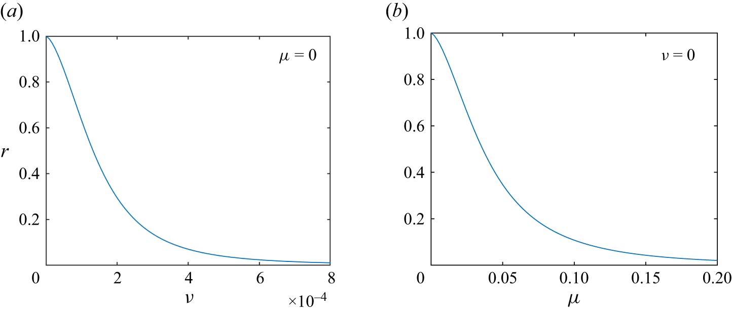
, indicating that flows with stronger dissipation have weaker wave–mean correlation. An example showing this trend is plotted in figure 3. Interestingly,
 $\beta$
and the forcing strength
 $\sigma$
do not appear in the expression (3.23), although they do play a role in the correlation through affecting the growth rate
 $s$
, given by (2.20).
Variation of
 $r$
with
 $\mu$
and
 $\nu$
at
 $\beta =5$
,
 $\sigma =0.05$
,
 $m=8$
,
 $k=16$
. Here,
 $s$
is computed using the dispersion relation (2.20).

Figure 3. Long description
Two panels show (a) the variation of the coefficient (r) with viscosity (nu) for zero drag (mu), (b) the variation of the coefficient (r) with drag (mu) for zero viscosity (nu). In both cases the coefficient (r) decreases from one to zero.
We can further deduce from (3.23) that, in general,
 \begin{equation} 0\lt r\lt 1. \end{equation}
The
 $r\rightarrow 0$
limit is achieved as
 $\nu \rightarrow \infty$
or
 $\mu \rightarrow \infty$
. In practice,
 $r$
becomes negligible only when
 $\mu$
or
 $\nu k^2\gtrsim 0.2$
, which yields
 $r\lesssim 0.02$
(cf. figure 3). The decorrelation assumption (2.17) is justified in this limit, but because the zonal flow is strongly damped (
 $s\rightarrow -\mu -\nu m^2$
), it is not relevant to zonostrophic instability. The
 $r\rightarrow 1$
limit is achieved as
 $\nu \rightarrow 0$
and
 $\mu \rightarrow 0$
. In practice,
 $r\gtrsim 0.97$
when
 $\mu$
or
 $\nu k^2$
falls below
 $2\times 10^{-3}$
, which makes the zonostrophic instability strong. Since
 $r$
is no longer small, (3.23) may not be accurate for the correlation in this limit, but we may still infer significant correlation given the pronounced inconsistency of the decorrelation assumption.
The condition of neutral stability
 $s=0$
is of special interest as it heralds the onset of instability, and we conclude this section by looking at the value of
 $r$
in this case. If there is only drag and no viscosity, then
 \begin{equation} r=\frac {1}{3},\quad \mathrm{for} \quad s=0,\quad \nu =0. \end{equation}
Since the value
 $1/3$
is not a very small number, in this case the wave–mean correlation is already significant at the onset of instability. On the other hand, if there is only viscosity and no drag, then
 \begin{equation} r=\frac { m^2}{ 2k^2+m^2},\quad \mathrm{for} \quad s=0,\quad \mu =0. \end{equation}
We find that the instability is most prominent when
 $m\sim k/2$
(cf. figure 4 shown later), which implies
 $r\sim 1/9$
. This smaller value indicates that, when viscosity dominates the dissipation, the wave–mean correlation is weak at the onset of instability. This indicates that stronger wave–mean correlations are generated under drag than under viscosity, which is consistent with the greater stochasticity that is seen for drag compared with viscosity in figures 2
 $(a$
) and 2(
 $d)$
.


It would be interesting to validate the results of the correlation via numerical simulations. However, we found that the coupling term between the wave and mean flow,
 $\hat {U}(\tau )\hat {\psi }_1(\tau )\hat {\psi }_1^*(t)$
in (3.18) is extremely stochastic; even an ensemble average over 1000 realisations does not converge to a reliable approximation for its expectation. We have confirmed that such an enhanced stochasticity results from the coupling of the wave and the mean flow, as it is stronger than the stochasticity of either separately. These findings are documented in Appendix A. It is thus too challenging for us to find the value of
 $r$
from stochastic simulations. To validate the theory, we will instead consider the effect of the correlation on the growth rate of the mean flow, which can be effectively extracted from the stochastic simulations, as we will demonstrate in the next section.
3.3. Effect on the growth rate
The wave–mean correlation will have an impact on the growth rate of zonostrophic instability. The derivation of the dispersion relation (2.20) has assumed zero correlation, and we have shown that the correlation modifies the dispersion relation through (3.21). We now study the impact of the correlation on the growth rate of the instability. Substituting the leading-order correlation (3.23) into (3.21), we have
 \begin{equation} s+\mu +\nu m^2=\frac {m^2\sigma ^2\varLambda }{2k^2(\mu +\nu k^2)}\left (\frac {1}{s-\lambda _1^*-\lambda _2}+\frac {1}{s-\lambda _1-\lambda _2^*}\right )\left [1+\frac {s+\mu +\nu m^2}{s+3\mu +\nu (2k^2+m^2)}\right ]\!. \end{equation}
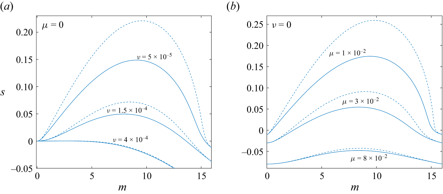
This is an improved dispersion relation over (2.20), which we now term the original dispersion relation. In figure 4, we plot an example for the original and improved dispersion relations in solid and dashed lines, respectively. Because
 $r\gt 0$
, the improved dispersion relation predicts a higher growth rate than the original dispersion relation, and the difference between the two growth rates becomes larger as the instability grows stronger due to larger values of
 $r$
.
To validate the theory, we compute the ensemble average of
 $\hat {U}$
, denoted
 $\langle \hat {U} \rangle$
, for each set of 100 stochastic simulations shown in figure 2, as an approximation to the expectation
 $\mathbb{E}[\hat {U}]$
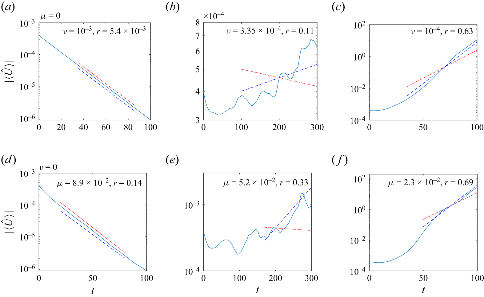
, and then compare this with the theoretical growth rates. This comparison is shown in figure 5. The red dash–dot lines and the blue dashed lines represent the growth rates of the original and improved dispersion relations, respectively. For panels
 $(a)$
and
 $(d)$
where strong dissipation suppresses instability, the value of
 $r$
is small. Consequently, the decay rates from (2.20) and (3.27) are nearly the same, both exhibiting good agreement with the simulations. In panels
 $(b)$
and
 $(e)$
, the dissipation becomes weaker, both corresponding to marginal instability with a very small decay rate of
 $s=-9\times 10^{-4}$
predicted by the original dispersion relation. The improved dispersion relation, on the other hand, predicts an exponential growth. The numerical simulations demonstrate considerable stochasticity in these two cases, but the exponential growth is apparent, and the general trend is more or less described by the improved dispersion relation. We note that the difference between the two dispersion relations is much larger for panel
 $(e)$
than panel
 $(b)$
, in agreement with the discussion around (3.25) and (3.26) that drag yields stronger wave–mean correlation at instability threshold. Finally, in panels
 $(c)$
and
 $(f)$
, dissipation is further reduced resulting in significant instability. The improved dispersion relation predicts a higher growth rate than the original counterpart, and demonstrates better agreement with the simulations.
Ensemble average of stochastic realisations in figure 2 compared with the theory. The red dash–dot lines represent the growth rates of the original dispersion relation (2.20), and the blue dashed lines represent the growth rates of the improved dispersion relation (3.27).

Figure 5. Long description
The image contains six line graphs labeled (a) through (f), each comparing growth rates of dispersion relations with stochastic realizations. Panel A: A line graph with the y-axis labeled |Ū| and the x-axis labeled t. The graph shows a decreasing trend with three lines: a solid blue line, a dashed blue line, and a dash-dot red line. The values of μ, ν, and r are provided in the legend. Panel B: A line graph with the y-axis labeled in units of 10^-4 and the x-axis labeled t. The graph shows an increasing trend with three lines: a solid blue line, a dashed blue line, and a dash-dot red line. The values of ν and r are provided in the legend. Panel C: A line graph with both axes on a logarithmic scale, labeled t and |Ū|. The graph shows an increasing trend with three lines: a solid blue line, a dashed blue line, and a dash-dot red line. The values of ν and r are provided in the legend. Panel D: A line graph with the y-axis labeled |Ū| and the x-axis labeled t. The graph shows a decreasing trend with three lines: a solid blue line, a dashed blue line, and a dash-dot red line. The values of μ, ν, and r are provided in the legend. Panel E: A line graph with both axes on a logarithmic scale, labeled t and |Ū|. The graph shows an increasing trend with three lines: a solid blue line, a dashed blue line, and a dash-dot red line. The values of μ and r are provided in the legend. Panel F: A line graph with both axes on a logarithmic scale, labeled t and |Ū|. The graph shows an increasing trend with three lines: a solid blue line, a dashed blue line, and a dash-dot red line. The values of μ and r are provided in the legend.
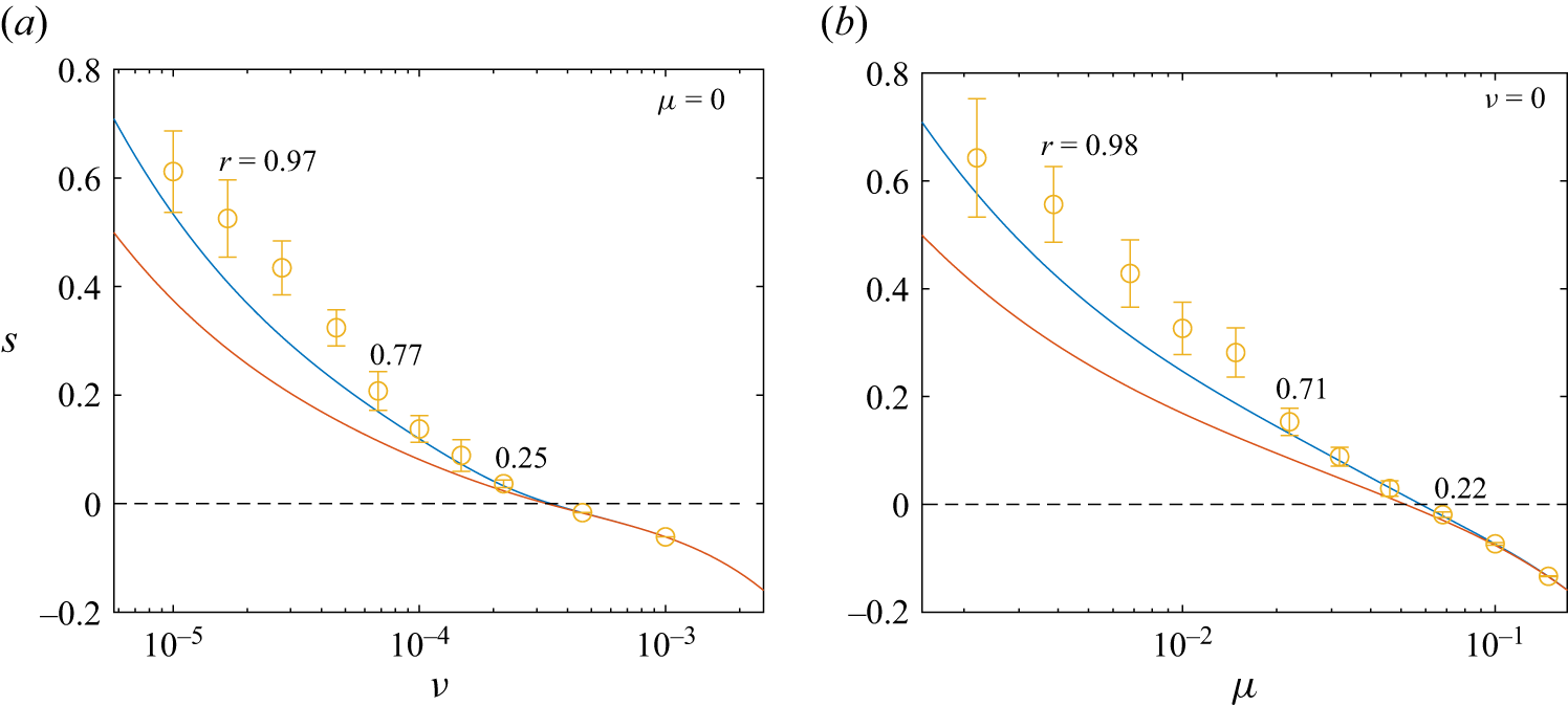
In figure 6, we measure the growth rates from stochastic simulations and compare with the theory. For each condition, we perform 1000 realisations and take the ensemble average
 $\langle \hat {U}\rangle$
. We then undertake a linear regression for the logarithm of
 $|\langle \hat {U}\rangle |$
in the time period
 $t\in [100,200]$
(chosen as a representative time interval over which majority of the simulations exhibit exponential growth or decay). Although we have increased the number of realisations to 1000, their ensemble average still exhibits considerable stochasticity. We thus repeat this procedure 20 times to obtain 20 growth rates, and then compute their mean and standard deviation, which are plotted as error bars in figure 6. We may interpret the standard deviation of growth rates as an indicator for the extent of stochasticity. We also give some numerical values of
 $r$
for representative values of
 $\nu$
and
 $\mu$
. For strong dissipation with
 $r\lesssim 0.2$
, the growth rates of simulations exhibit very small error bars and agree well with both the dispersion relations. As the dissipation is reduced so that
 $r\gtrsim 0.2$
, the error bars for the growth rate become more clearly visible and the two dispersion relations diverge, implying a stronger extent of stochasticity. While the original dispersion relation underestimates the growth rates predicted by the simulations, the improved dispersion relation provides good agreement up to
 $r\sim 0.7$
. As
 $r$
further increases, the error bar for the growth rates becomes more prominent and the improved dispersion relation also underestimates the actual growth rates, but overall it still predicts the general trend reasonably well.
Growth rates measured from numerical simulations (error bars) compared with the original dispersion relation (red lines) and the improved dispersion relation (blue lines),
 $\beta =5$
,
 $\sigma =0.05$
,
 $k=16$
,
 $m=8$
.

We have shown that the improved dispersion relation indeed provides much more accurate growth rates than the original one. However, we also note that the original dispersion relation makes sense qualitatively, i.e. the growth rate it predicts is of the correct order of magnitude. This is related to the fact that the value of
 $r$
representing the inconsistency of the decorrelation assumption never gets large (cf. (3.24)), hence the assumption never gets growth rates ‘very wrong’.
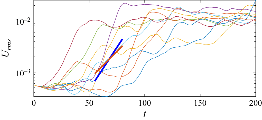
We now compare the theory with the numerical solutions of the full nonlinear equation (2.1). We run ten nonlinear simulations for the same parameters as in figure 1 and compute the r.m.s. zonal flow
 $U_{\textit{rms}}$
, defined in (2.8). The results are plotted in figure 7. We also plot the exponential growth of the theory in thick lines: the red and blue thick lines represent the results of the original and the improved dispersion relation, respectively. We see that, while all realisations demonstrate prominent exponential growth, there are considerable differences between different realisations, as well as differences in one realisation at different times, confirming that the zonal mean flow is stochastic in nonlinear simulations as well. To compare the theory and the simulations, the ensemble mean of the simulation results may not appropriately represent the linear instability because, in a given time interval, some realisations have reached nonlinear saturation while others have not yet started to grow exponentially. Instead, we directly compare the theory with individual simulations. If we look at the time period when a realisation is experiencing exponential growth, we see that the growth of most realisations is faster than that predicted by the original dispersion relation. The growth rate from the improved dispersion relation, on the other hand, lies between the fastest and slowest growth rates among various realisations, and seems to more or less agree with the growth in several simulations. The improved dispersion relation therefore better describes the exponential growth seen in the nonlinear simulations.
Evolution of
 $U_{\textit{rms}}$
in ten realisations for the same parameter regime as figure 1 plotted in ten curves. The red and blue thick lines represent the exponential growth of the original and improved dispersion relation, respectively.

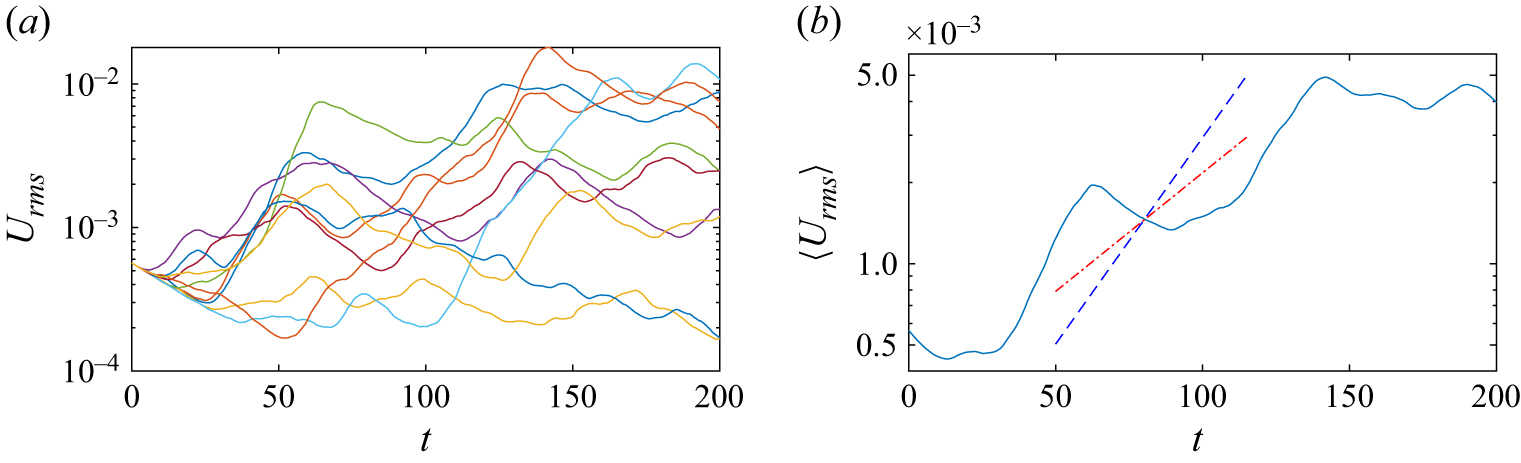
More quantitative comparisons between the theory and simulations can be made at stronger dissipations. In figure 8, we increase the drag coefficient from
 $\mu =0.01$
to
 $\mu =0.023$
, and show the evolution of ten realisations in panel
 $(a)$
. The stronger dissipation allows a longer time period for the instability to saturate, during which more realisations show a clear window of exponential growth. The ensemble mean of the simulations thus allows a closer comparison with the theoretical dispersion relations, as shown in panel
 $(b)$
. We see that there are two prominent periods of exponential growth. For each of them, the improved dispersion relation (the blue dashed line) yields better agreement with the simulations compared with the original dispersion relation (the red dash–dot line) which underestimate the growth. The effect of wave–mean correlation on the growth rate has thus been confirmed in nonlinear simulations.
Numerical solutions of equation (2.1) compared with the theory of zonostrophic instability at
 $\mu =0.023$
(the other parameters are the same as in figure 1). Panel
 $(a)$
plots the results of ten stochastic simulations. Panel
 $(b)$
plots their ensemble average compared with the original dispersion relation (the red dash–dot line) and the improved dispersion relation (the blue dashed line).

We note that the quasi-linear approximation, which we used at the outset in our theoretical development (see (2.10, 2.11)), could also affect the comparison with the full simulations. Our preliminary analysis suggests that the quasi-linear approximation yields accurate results for zonostrophic instability if the forcing is weak and
 $\beta$
is relatively large, which is satisfied by our choice of parameters,
 $\sigma =0.05$
,
 $\beta =5$
.
4. Conclusions and remarks
In this paper, we have studied the stochasticity of zonal mean flows in zonostrophic instability, the phenomenon that in a stochastically forced wave field, weak zonal mean flows grow exponentially to form strong zonal jets. The stochasticity of zonal mean flows is often neglected in reduced models based on the statistics of turbulence, which we term the deterministic mean-flow assumption, following an ergodic assumption that the zonal mean equals the ensemble mean. However, by carrying out a large number of simulations, we showed that the zonal mean flow generally experiences a significant degree of stochasticity. We then studied the impact of this stochasticity on zonostrophic instability. We demonstrated that the actual assumption needed for the analysis of zonostrophic instability is weaker than the deterministic mean-flow assumption: in fact, we only need to assume that the waves and the mean flow are statistically decorrelated. We term this assumption the wave–mean-flow decorrelation assumption, or the decorrelation assumption for short. We examined this assumption theoretically and, using the evolution equation for the zonal mean flow, we derived an analytical expression for weak correlation between waves and mean flows. Results indicate that the correlation becomes stronger as the instability gets stronger, and it is generally significant when the instability is prominent. The wave–mean correlation results in a higher growth rate of the zonostrophic instability. An improved dispersion relation based on this correlation is derived, which proves to be much more accurate. Results also indicate that, while the wave–mean correlation has a significant impact on growth rates in general, the correction never becomes large. As a result, the theory derived under the decorrelation assumption predicts growth rates of the right order of magnitude. We also found that bottom drag results in stronger mean-flow stochasticity and wave–mean correlation than dissipation through viscosity. The theoretical predictions were verified by numerical simulations based on stochastic ODEs and full nonlinear partial differential equations.
Several new topics are promising for future research. The present study considered a forcing with a single wavevector, which is highly anisotropic. A more isotropic forcing, which is more realistic in geophysical and astrophysical settings, would be desirable. Our preliminary analysis indicates that, when the forcing contains wavevectors in multiple directions,
 $\beta$
usually appears explicitly in the expression for wave–mean correlation and it would therefore be interesting to explore its role. The effect of a magnetic field is another interesting topic. The numerical simulations of Wang et al. (Reference Wang, Mason and Gilbert2024) showed that magnetic fields can significantly enhance the extent of mean-flow stochasticity. It is therefore anticipated that a magnetic field can also lead to considerable wave–mean correlations and thus have a strong impact on growth rates.
Our results could have implications on a number of related studies in the literature. The theories of SSST, CE2 and DSS with a zonal average have also used the ergodic assumption, resulting in the deterministic mean-flow assumption. Since our study reveals that the effects of mean-flow stochasticity can be significant, it is reasonable to question its role in these theories as well. We note that, to improve the accuracy of DSS based on CE2, many efforts have been made to improve the quasi-linear approximation via incorporating large-scale non-zonal components (Marston et al. Reference Marston, Chini and Tobias2016; Tobias et al. Reference Tobias, Oishi and Marston2018; Nivarti et al. Reference Nivarti, Marston and Tobias2025b ). Our study, on the other hand, has demonstrated the necessity to examine the effect of the ergodic assumption.
Since Allawala et al. (Reference Allawala, Tobias and Marston2020) have shown that CE2 with ensemble average produces more accurate results than the zonal average, it would be interesting to probe the theory of zonostrophic instability using the ensemble average, where the role of wave–mean correlation could also be important. Very recently, Nivarti et al. (Reference Nivarti, Kerswell, Marston and Tobias2025a ) showed the non-equivalence between quasi-linear dynamical systems and their statistical closures. They found that performing CE2 with a zonal average on quasi-linear systems results in spurious new instabilities due to an increase of dimension, which they term ‘rank instability’. Since the statistical closure used to obtain CE2 with a zonal average is the ergodic assumption, which we have found does not hold in general, our present paper provides another concrete example for such non-equivalence. We note that, in rank instability, such non-equivalence happens in spatial harmonics which are much weaker than the zonal mean flow that we study here, thus failure of the ergodic assumption may have a more significant impact.
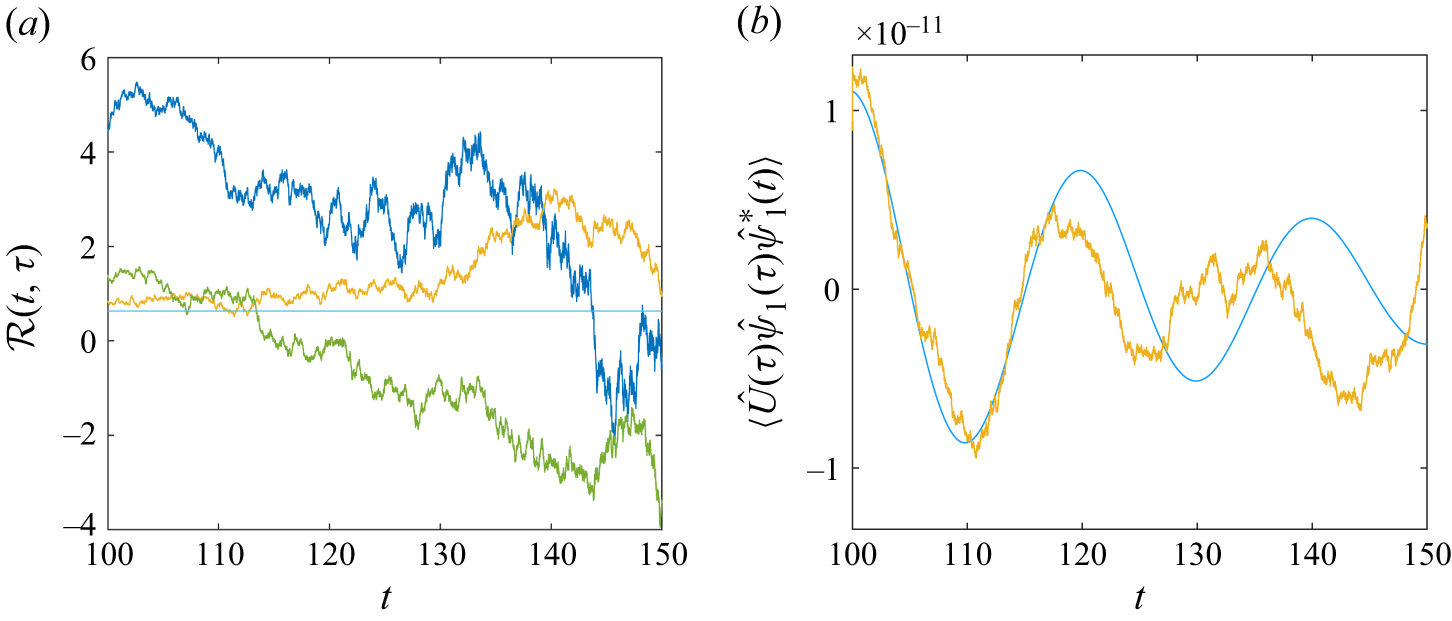
 $(a)$
The real part of
 $\mathcal{R}(t,\tau )$
computed from stochastic simulations with
 $\tau =100$
and the same parameters as figure 5
 $(c)$
. Each of the three curves is obtained from an ensemble average of 1000 simulations. The horizontal line represents the theoretical value
 $r=0.63$
.
 $(b)$
The evolution of the real part of
 $\langle \hat {U}(\tau )\hat {\psi }_1(\tau )\hat {\psi }_1^*(t)\rangle$
(yellow curve) corresponding to the yellow curve in panel
 $(a)$
, and the theoretical expectation (blue curve).

Acknowledgements
We thank Dr X. Du for providing references discussing the expectation of quartic products of white noise. We thank the referees for constructive comments that have significantly improved the quality of the paper.
Funding
C.W. acknowledges the start-up fund for young scholars offered by Beijing Normal University (grant 312200502507) and Beijing Normal–Hong Kong Baptist University (grant UICR0700081-24). This work was initiated under EPSRC grant EP/T023139/1, which C.W., A.D.G. and J.M. gratefully acknowledge.
Declaration of interests
The authors report no conflict of interest.
Data access statement
The numerical code used to perform the simulations in figures 1, 2, 5, 6, 7, 8, 9 is available at https://github.com/Chen-UIC/Stochasticity-of-zonostrophic-instability .
Appendix A. Numerical simulation of the wave–mean correlation
We have tried to compute the correlation (3.18) through stochastic simulations via
 \begin{equation} \mathcal{R}(t,\tau )=\frac { \langle \hat {U}(\tau )\hat {\psi }_1(\tau )\hat {\psi }_1^*(t)\rangle -\langle \hat {U}(\tau )\rangle \, \langle \hat {\psi }_1(\tau )\hat {\psi }_1^*(t)\rangle }{\langle \hat {U}(\tau )\rangle \, \langle \hat {\psi }_1(\tau )\hat {\psi }_1^*(t)\rangle }, \end{equation}
where an angled bracket represents an ensemble average. Results of the real part of
 $\mathcal{R}(t,\tau )$
with
 $\tau$
fixed at 100 are shown in figure 9
 $(a)$
. Each of the three curves is computed through an ensemble average of 1000 stochastic simulations, and the theoretical result of
 $r=0.63$
is plotted as a horizontal line. Even with 1000 stochastic simulations,
 $\mathcal{R}$
exhibits considerable stochasticity, represented by the difference between the three curves, and the random fluctuations with time. Such strong stochasticity makes comparison with the theoretical value of
 $r$
difficult. It is impractical to further increase the number of realisations to make
 $\mathcal{R}(t,\tau )$
converge to meaningful results.
The strong stochasticity of
 $\mathcal{R}(t,\tau )$
is caused by the coupling term
 $\langle \hat {U}(\tau )\hat {\psi }_1(\tau )\hat {\psi }_1^*(t)\rangle$
. In figure 9
 $(b)$
, we plot
 $\langle \hat {U}(\tau )\hat {\psi }_1(\tau )\hat {\psi }_1^*(t)\rangle$
corresponding to the yellow curve in figure 9
 $(a)$
, along with its theoretical expectation (the smooth curve) which follows
 \begin{equation} \mathbb{E}\bigr [\hat {U}(\tau )\hat {\psi }_1(\tau )\hat {\psi }_1^*(t)\bigr ]\sim e^{\lambda _1^*(t-\tau )+s\tau }. \end{equation}
We see that
 $\langle \hat {U}(\tau )\hat {\psi }_1(\tau )\hat {\psi }_1^*(t)\rangle$
does not converge well to the expectation even with 1000 realisations. This is quite different from the mean flow
 $\hat {U}(t)$
: as we have shown in figure 5
 $(c)$
, although
 $\hat {U}(t)$
is also stochastic during the instability, an ensemble average of 100 realisations converges well to its expectation. We have verified that the wave term
 $\hat {\psi }_1(\tau )\hat {\psi }_1^*(t)$
behaves similarly with much weaker stochasticity: merely 20 realisations yield good agreement with the expectation.
The enhanced stochasticity of
 $\hat {U}(\tau )\hat {\psi }_1(\tau )\hat {\psi }_1^*(t)$
is therefore caused by the coupling between the wave and the mean flow. We may understand this from the theory for products of random variables. For example, Goodman (Reference Goodman1962) has derived the variance of products of multiple random variables, which is shown to be related to the product of variance of individual random variables. We can thus infer that multiplying two random variables together results in a much higher stochasticity. It is an interesting topic for future research to further explore the nature of this strong stochasticity, as well as numerical methods to effectively compute the expectation.

 ψ=εcosmy
 t=0
 β=5
 ν=10−4
 μ=0.01
 σ=0.05
 k=16
 m=8
 ε=10−4
 (a)
 ζ(x,y,t)
 (b)
 U(y,t)
 t
 (c)
 U(t,y)
 (d)
 Urms(t)
 β=5
 σ=0.05
 k=16
 m=8
 (a
 c)
 μ=0
 (d
 f)
 ν=0
 (a)
 (d)
 s=−0.061
 (b)
 (e)
 s=−9×10⁻⁴
 (c)
 (f)
 s=0.081
 r
 μ
 ν
 β=5
 σ=0.05
 m=8
 k=16
 s
 β=5
 k=16
 σ=0.05
 β=5
 σ=0.05
 k=16
 m=8
 Urms
 μ=0.023
 (a)
 (b)
 (a)
 R(t,τ)
 τ=100
 (c)
 r=0.63
 (b)
 ⟨U^(τ)ψ^1(τ)ψ^1∗(t)⟩
 (a)


