Implications
All the indices that have been proposed so far to characterize animal sociability require the whole group to be observed. Advances in the automatic recording of animal distribution using telemetry collars can contribute to low-cost acquisition of quantitative information, but this is limited by breakdown of telemetry collars and by the number of available collars. We therefore propose an index for analysing variations in affinity relationships within groups of domestic herbivores, whose definition does not depend on group size and that can be computed if not all the animals are observed at each date.
Introduction
Analysing variations in affinity relationships within groups of domestic herbivores has implications for animal welfare (i.e. limitation of agonistic interactions) in intensive production systems and for grassland use in the more extensive systems. In such grassland-based systems, managers would benefit from understanding and manipulating livestock grazing patterns to limit resource degradation and preserve biodiversity. Continued research at both theoretical and applied levels is thus needed (Bailey et al., Reference Bailey, Dumont and Wallis De Vries1998; Boval and Dixon, Reference Boval and Dixon2012; Swain and Friend, Reference Swain and Friend2013). In groups of domestic herbivores, sociability describes the motivation of individuals to remain close to conspecifics. Affinity relationships based on positive interactions ensure group cohesion and increase social tolerance in conflict situations (Bouissou et al., Reference Bouissou, Boissy, Le Neindre and Veissier2001). Although less studied than the impact of agonistic interactions, these ‘positive’ social interactions influence a large range of individual behaviours (Rault, Reference Rault2012), including grazing distribution (Howery et al., Reference Howery, Provenza, Banner and Scott1998; Boissy and Dumont, Reference Boissy and Dumont2002; Sibbald et al., Reference Sibbald, Oom, Hooper and Anderson2008). Defining and measuring variability in affinity relationships in domestic herbivores can thus help in understanding the temporal dynamics of group organization and its consequences on grazing distribution.
Sociability has been described in various ways, depending on the aims of the studies and how observations were carried out; many of them can be found in SOCPROG, a set of programmes for analysing data on animal associations and social structures (Whitehead, Reference Whitehead2009). For instance, operant conditioning has been used at an individual level for measuring how hard animals will work to gain access to conspecifics (Holm et al., Reference Holm, Jensen and Jeppesen2002), and behavioural responses to isolation were frequently recorded in arena tests (Hopster and Blokhuis, Reference Hopster and Blokhuis1994; Gibbons et al., Reference Gibbons, Lawrence and Haskell2010; Ligout et al., Reference Ligout, Foulquié, Sèbe, Bouix and Boissy2011). Ramseyer et al. (Reference Ramseyer, Boissy, Dumont and Thierry2009a and 2009b) measured affinities between individuals by recording positive interactions in each pair (i.e. licking and rubbing with or without soliciting) with all-occurrence sampling. Aschwanden et al. (Reference Aschwanden, Gygax, Wechsler and Keil2008) recorded all possible pairs within a goat herd, and concluded that dyads with positive interactions showed smaller distances than neutral or agonistic dyads. At the group level, affinities were also measured based on analyses of variations in inter-individual distances (Arnold and Dudzinski, Reference Arnold and Dudzinski1978; Boissy and Dumont, Reference Boissy and Dumont2002). Freire et al. (Reference Freire, Swain and Friend2012) recorded relative positions between pairs of individuals using a proximity logger that records the amount of time that each sheep spent within 4 m of group members. Affinities were calculated based on the identification of individuals encountered within 4 m and the number and duration of any encounter. In dairy cows, Gibbons et al. (Reference Gibbons, Lawrence and Haskell2010) reported consistency between individual response to isolation and the frequency of recordings with two close neighbours (i.e. <1 m away) in their home-pen. Sibbald et al. (Reference Sibbald, Elston, Smith and Erhard2005) defined a sociability index, which is equivalent to the relative proportion of time each individual of a group is recorded as the nearest neighbour of any group-mates. The method ignored arbitrary distance thresholds as, at pasture, the spatial distribution of animals can vary with external factors such as herbage availability. Ligout et al. (Reference Ligout, Foulquié, Sèbe, Bouix and Boissy2011) showed that the inter-individual variance of Sibbald sociability index could be related to the behaviour of animals during the isolation phase of an arena test (i.e. based on vocalization frequency and locomotor behaviour). At pasture, sheep with the lowest sociability index were also those that more readily moved away from familiar parked peers to express a food preference (Sibbald et al., Reference Sibbald, Erhard, Hooper, Dumont and Boissy2006). Recently, Della-Rossa et al. (Reference Della-Rossa, Chadœuf, Boissy and Dumont2013) calculated Sibbald sociability index in two groups of grazing heifers, and showed that it gave consistent information compared with all occurrence sampling of positive interactions.
From a statistical point of view, it is noteworthy that there is no unique statistical model proposed by SOCPROG (Whitehead, Reference Whitehead2009). There are indeed two main options. If data are available for several groups, a global summary statistics can be built for each group that is analysed using classic methods such as regressions or ANOVA (Swain and Bishop-Hurley, Reference Swain and Bishop-Hurley2007). Conversely, if all data come from the same group, the preceding methods fail and hypothesis testing is based on permutation or bootstrap methods (e.g. Bejder et al., Reference Bejder, Fletcher and Brager1998). These methods can also be adapted to take into account various biological constraints (Whitehead, 1999; Peyrard et al., Reference Peyrard, Calonnec, Bonnot and Chadœuf2005; Swain and Bishop-Hurley, Reference Swain and Bishop-Hurley2007).
Methods based on all-occurrence sampling of affinity relationships require close monitoring of animal behaviour as data such as animal orientation, head movements, and positive or agonistic interactions are usually used as cues (Aschwanden et al., Reference Aschwanden, Gygax, Wechsler and Keil2008; Ramseyer et al., 2009Reference Ramseyer, Boissy, Dumont and Thierrya and 2009Reference Ramseyer, Thierry, Boissy and Dumontb). These methods are time consuming, whereas inter-individual distances or nearest-neighbour distributions could simply be obtained through the automatic recording of animal distribution using global positioning system (GPS) telemetry collars (Schlecht et al., Reference Schlecht, Hülsebusch, Mahler and Becker2004; Swain and Friend, Reference Swain and Friend2013) or proximity loggers (Freire et al., Reference Freire, Swain and Friend2012, Watson-Haigh et al., Reference Watson-Haigh, O’Neill and Kadarmideen2012). Proximity loggers require each sheep to be fitted with a neck collar recording all individuals within a fixed radius so that missing data will occur as soon as any logger fails in emission and reception. In addition, even if one is interested in pairs of animals, the whole group needs to be observed. This is clearly stated in the method proposed by Sibbald et al. (Reference Sibbald, Elston, Smith and Erhard2005), which is suitable for groups of animals in which all individuals are visible and identifiable to record which animal is the nearest neighbour of any other one. The same constraint appears in the method proposed by Solanas et al. (Reference Solanas, Salafranca, Riba, Sierra and Leiva2006), who used the asymmetry of social relationships from nearest-neighbour matrices for analysing dyadic interactions in a social system. In addition, when all positive interactions were recorded (Ramseyer et al., Reference Ramseyer, Boissy, Dumont and Thierry2009a and 2009Reference Ramseyer, Thierry, Boissy and Dumontb; Della-Rossa et al., Reference Della-Rossa, Chadœuf, Boissy and Dumont2013), the information was then summarized in a matrix in which all the animals were identified in rows and columns.
The necessity to identify each individual obviously limits the use of these methods in large groups. In addition, affinities were always compared inside a group, as they are based on inter-individual relationships within this group, and on probabilities for an animal to be at a given position with respect to another one. The apparent attachment of an individual to its group is likely to vary not only according to group composition (Sibbald et al., Reference Sibbald, Elston, Smith and Erhard2005) but also group size, which prevents any comparison between the groups. Here, we aim to propose an index for analysing variations in affinity relationships within groups of domestic herbivores, (i) based on the distance between individuals so that it can be obtained from automatic telemetry collars, (ii) which can be calculated when only some of the animals are monitored (i.e. in large herds where there are more individuals to be observed than available telemetry collars), (iii) which can be computed if not all the animals are observed at each date (i.e. to account for random breakdown of telemetry collars) and (iv) which allows comparing variability in affinity relationships between groups of different sizes. The proposed index and its estimators are presented before being compared with Sibbald sociability index that we considered as the reference method. We then illustrate its use on the basis of a case study with grazing heifers by investigating changes in the variability of affinities according to group size.
General methods
Sibbald sociability index
Consider a group of n animals observed at T dates, and denote
 $x_{{i,t}} $
the position of animal i at date t. The Sibbald index (Sibbald et al., Reference Sibbald, Elston, Smith and Erhard2005) is based on the estimation of the probability that j is the nearest neighbour of i, denoted
 $ P(j{\mid}i)$$
in the following, whose estimator is
 $$\mathord \hat P} \left( j{\mid}i \right)= $
 ${1 \over T}\sum_{{t{\les} T}} 1_{{\{\left|\,\mid\, {x_{{i,t}} {\minus}x_{{j,t}} } \mid \,\right |}\, =\, min_{k} (\,\mid\,\left| {x_{{i,t}} {\minus}x_{{k,t}} } \right|\,\mid\,)\} }} $$
. In the formula,
 $1_{{\{ C\} }} $
is the function whose value is 1 if condition C is true, 0 if it is false, so that
 $$\sum_{{_{{t\les T}} }} 1_{{\{ \left| {\left\mid{x_{{i,t}} {\minus}x_{{j,t}} } \mid \right} \right|=min_{k} (\,\mid\,\left| {x_{{i,t}} {\minus}x_{{k,t}} } \right|\,\mid\,)\} }} $$
counts how many times j was the nearest neighbour of i. The sociability index of animal i is then defined as
 $$SI\left( i \right)=\sum_{{j\,\ne\,i}} P(j{\mid}i)$$
. An animal in the centre of the group has statistically a larger SI than an animal at the edge of the group. A measure of sociability variability inside the group can be the variance of
 $P{\rm ( }j{\mid}i)$$
.
Proposed affinity index
Sibbald et al. (Reference Sibbald, Elston, Smith and Erhard2005) method depends on the estimation of
 $ P(j{\mid}i)$$
,and hence it depends on the measure of the relative positions between animals. Thus, this method cannot be used if some animals are missing. If some animals are missing, we propose to rather use a relative measure, that is, a function which measures how frequently an animal is closer than another one from a third animal. We therefore propose to use p(i,j|k), the probability that the distance between i and the focal animal k is smaller than the distance between j and k, assuming that an animal that is further away from the focal animal is less likely to be interacting with it. Several indices can then be defined according to the level at which one wants to estimate affinity:
-
∙ At the lowest level, one can look at affinity variations at the triplet level, that is, use
 $U\left( {i,j{\rm \,\mid\,}k} \right)=p(i,j \!\mid \! k)$
to measure affinity variations between i and j with respect to k.
-
∙ To calculate how frequently animal i is closer to the focal animal k than any other animal, one can then take the mean over j of the index computed on triplets,
$U\left( {i{\rm \,\mid\,}k} \right)={1 \over {n{\minus}2}}\sum_{{j\notin\{ i,k\} }} p(i,j\!\mid\!k)$
, where n denotes the size of the group. The matrix with elements U(i|k) is comparable to the affinity matrix of Sibbald. -
∙ At the highest level, one can compute U g , the variance of the p(i,j|k) to estimate variability in the strength of affinities within the group. U g is similar to the variance of the affinity matrix of Sibbald that allows estimating variability in affinity relationships within the group.


Estimating the index if no animal is missing
Suppose that the observation dates are distant enough so that they can be considered as independent and that all animals are observed at each date
 $ t \les T$$
where T is the total number of observation dates.
-
∙ The affinity relationship between i and k relatively to that between j and k is estimated as the proportion of observations when i is closer to k than to j:
$$\mathord\hat U} \left( {i,j{\rm \,\mid\,}k} \right)={1 \over T}\sum_{{t\les T}} 1{}_{{\{ \,\mid\,\left| {x_{{i,t}} {\minus}x_{{k,t}} } \right|\,\mid\,\les \,\mid\,\left| {x_{{j,t}} {\minus}x_{{k,t}} } \right|\,\mid\,\} }}$$
. It is unbiased, that is, its expectation is equal to the theoretical value U(i,j|k). Its variance is
$p\left( {i,j{\rm \,\mid\,}k} \right)(1{\minus}p\left( {i,j{\rm \,\mid\,}k} \right))/T$
. -
∙ Thus, estimators
$\mathord \hat U} (i\!\mid\!k)$
obtained by replacing the p(i,j|k) by their estimators are also unbiased. -
∙ An estimator A of the global variance of affinities in the group can be obtained by replacing the p(i,j|k) by their estimators. It has an expectation equal to
${1 \over {n\left( {n{\minus}1} \right)(n{\minus}2)}}$
$\sum_{{i\,\ne\,j,i\,\ne\,k,j\,\ne\,k}}({{p\left( {i,j{\rm \,\mid\,}k} \right)\left( {1{\minus}p\left( {i,j{\rm \,\mid\,}k} \right)} \right)} \over T}{\plus}(p\left( {i,j{\rm \,\mid\,}k} \right){\minus}1/2)^{2} )$
. Therefore, its bias
${1 \over {n\left( {n{\minus}1} \right)(n{\minus}2)}}\sum_{{i\,\ne\,j,i\,\ne\,k,j\,\ne\,k}} $
${{p\left( {i,j{\rm \,\mid\,}k} \right)\left( {1{\minus}p\left( {i,j{\rm \,\mid\,}k} \right)} \right)} \over T}$
tends to 0 when T tends to infinity. However, we propose to use
$\mathord \hat U} _{g} =A\,{\minus}\, {1 \over {n\left( {n{\minus}1} \right)(n{\minus}2)}}\sum_{{i\,\ne\,j,i\,\ne\,k,j\,\ne\,k}} {{p\left( {i,j{\rm \,\mid\,}k} \right)\left( {1{\minus}p\left( {i,j{\rm \,\mid\,}k} \right)} \right)} \over T}$
whose bias
${1 \over {n\left( {n{\minus}1} \right)(n{\minus}2)}}\sum_{{i\,\ne\,j,i\,\ne\,k,j\,\ne\,k}} {{p\left( {i,j{\rm \,\mid\,}k} \right)\left( {1{\minus}p\left( {i,j{\rm \,\mid\,}k} \right)} \right)} \over T^2}$
tends to be 0 faster with respect to the number of dates T.


Covariances between
 $\hat{U}(i,j\!\mid\!k)$
and Û(i′,j′|k′) cannot be analysed if (i,j,k)≠(i′,j′,k′), as it depends on the interaction model between animals that is not easy to compute even if animals are independent. Therefore, the distribution of these estimators and that of
 $\hat{U}_{g} $
can be obtained by a bootstrap method (Efron and Tibshirani, Reference Efron and Tibshirani1993) if T, the number of observation dates, is large enough.
Estimating the index if the same animals are always missing
If only a subset S of always the same m animals is observed at the T dates, these animals being chosen independently with equal probability:
-
∙ The estimators
$\hat{U}(i,j\!\mid\!k)$
can be computed if i, j and k belong to S.
-
∙
$U(i\!\mid\!k)$
can be estimated if i and k belong to S, using the other animals j
$ \in $$
S:
$$\hat{U}\left( {i{\rm \,\mid\,}k} \right)={1 \over {m\:{\minus}\:2}}\sum_{{j\in S\{ i,k\} }} \hat{U}(i,j\!\mid\!k)$$
. Animals j
$ \in $$
S: having been chosen independently among the n animals, then
$\hat{U}(i\!\mid\!k)$
is an unbiased estimator of
${1 \over {n{\minus}2}}\sum_{{j\notin\{ i,k\} }} p(i,j\!\mid\!k)=U(i\!\mid\!k)$
. -
∙
$ \hat{U}_{s} $
computed on the subset S is biased with speed 1/T
2 in the same way as for complete data.


Estimating the index if some recordings are randomly missing
If the subset of observed animals varies across measurement days, for instance, because of telemetry collar breakdown, the solution is to use the subset S t of the m t animals observed at each date. Then as before,
-
∙ The estimators
$\hat{U}(i,j\!\mid\!k)$
are unbiased for triplets i, j and k for whom there exists some dates where they are simultaneously observed. -
∙ The estimators
$\hat{U}(i\!\mid\!k)$
can be estimated if there exists at least one triplet i, j and k for whom there exists some dates at which they are simultaneously observed, as
$\hat{U}\left( {i{\rm \,\mid\,}k} \right)={1 \over {(m_{{i,k}} {\minus}2)}}\sum_{{j\in S_{{i,k}} }} \hat{U}(i,j\!\mid\!k)$
if S
i,k
denotes the subset of animals j such that (i, j, k) are simultaneously equipped at some dates and
$m_{{i,k}} $
denotes their number. Equipped animals having been chosen independently among the n animals, then Û(i|k) is an unbiased estimator of
${1 \over {n{\minus}2}}\sum_{{j\notin\{ i,k\} }} p(i,j\!\mid\!k)$
.


If T i,j,k denotes the number of dates when i, j and k are present simultaneously then:
 $$E(\hat{U}_{g} )={1 \over {n\left( {n{\minus}1} \right)(n{\minus}2)}}\sum_{{i\,\ne\,j,i\,\ne\,k\,\ne\,,j\,\ne\,k}}({{p\left( {i,j{\rm \,\mid\,}k} \right)\left( {1{\minus}p\left( {i,j{\rm \,\mid\,}k} \right)} \right)} \over {T_{{i,j,k}}^{2} }}{\plus}$
 $(p\left( {i,j{\rm \,\mid\,}k} \right){\minus}1/2)^{2} )$$
. Thus, same conclusions can be drawn as before when
 ${\rm min}(T_{{i,j,k}} )\to\infty$
, that is, when the number of observations of the least observed triplet tends to infinity.
Simulation study
The simulation study was carried out based on four different models of affinity relationships, using a Gibbs point process with a fixed number of points (Stoyan et al., Reference Stoyan, Kendall and Mecke1987), more precisely a point interaction model, to simulate independent replicates of the spatial locations of individuals. Basically, the probability density that the animals are at locations
 $(M_{{1,}} \,\ldots\,M_{I} )$
is proportional to
 $e^{{{\minus}\sum_{{i\,\ne\,j}} g(M_{i} {\minus}M_{j} )}} $
. The function g(d) describes the strength at which the two animals interact with respect to their separating distance d and is called the pair interaction potential.
-
∙ The first model, later called ‘random group’, runs without any affinity relationships so that animals are randomly distributed in the plot at each date.
-
∙ The second model, called ‘recently mixed group’, describes affinity relationships. We assume that the group is made of k subgroups of l animals. Two animals within each subgroup interact strongly with interaction potential g(d)=10 d2, whereas two animals from different subgroups interact weakly with interaction potential g(d)=0.1 d2. This situation corresponds to what could be observed after unfamiliar groups have been put together into a paddock, as it takes several weeks for sheep groups to become integrated, even if they are of the same sex and age (Arnold and Pahl, Reference Arnold and Pahl1974).
-
∙ The third model, called ‘family group’, considers affinities between an animal and l-1 peers. Interactions between this animal and its preferred peers are strong with interaction potential g(d)=10 d2, whereas interactions between two followers of the same group are medium with interaction potential g(d)=d2, and interactions between two animals of different subgroups are weak with interaction potential g(d)=0.1d2. This situation could correspond to a group made of k females with their l-1 daughters.
-
∙ The fourth model, called ‘lognormal group’, considers one group, in which interaction potentials between pairs of animals are fitted with a lognormal LN(2,0.5) distribution, which corresponds to a group of animals with similar characteristics but continuous distribution of affinities.
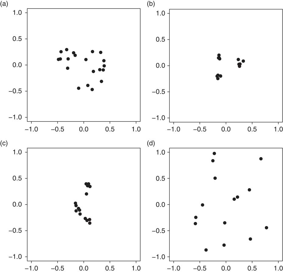
One hundred samples formed of up to 100 independent spatial location replicates were simulated for each model and each combination (n,k,l). Figure 1 shows typical examples of simulated spatial locations for groups of 21 animals.
Simulations of the locations of the animals of a group of 21 animals under independence assumption (a), under the assumption of a low dependence between three recently mixed groups of seven animals (b), under the assumption of three family groups of seven animals (c), and under the assumption of continuous distribution of affinities between animal pairs (d).

Comparison with Sibbald index
The comparison was made on groups of 12 animals, these groups being made of three subgroups in the recently mixed group and family group models, that is, for the second and third models. This number was chosen so as to get a minimal number of animals in interaction, allowing to test for the effects of removing between one and five animals; animal number was not too high, which allows measuring the consequences of individual effects.
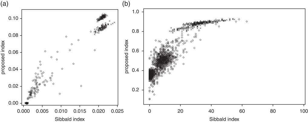
Figure 2a shows how the estimator
 $\hat{U}_{g} $
of the global variance of affinities in the group for complete data sets varies according to that calculated based on the Sibbald index (i.e. the variance of the affinity matrix for complete data sets). Circles corresponding to groups of independent animals are gathered around (0, 0), triangles and crosses corresponding to recently mixed and family groups are gathered around (0.021, 0.10) and (0.021, 0.09), whereas diamonds are spread between these extremes. Thus, the two estimators discriminated groups of independent animals from the groups organized into subgroups. The groups whose interactions are fitted with a lognormal distribution showed the largest variability. The relationship between Sibbald index and the proposed index was not linear as they did not measure the same characteristics.
Comparison between Sibbald and the proposed index. Comparison of global affinity indices (a) and the affinity coefficients between two animals (b), on 100 independent repetitions of groups of 12 animals observed at 100 dates. Circles: groups of independent animals; triangles: recently mixed groups; crosses: family groups; diamond: continuously distributed affinities.

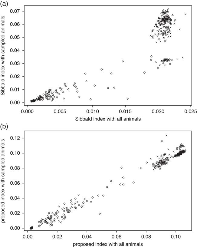
When only 8 of the 12 animals were observed in each simulation, the variance computed from Sibbald index diverged from that computed from the whole group according to group structure (Figure 3a) and which animals were sampled. Circles remain centred around (0, 0), whereas triangles and crosses groups are split in two subgroups centred on (0.21, 0.03) and (0.21, 0.06). If, for example, three from the four missing animals belong to the same subgroup (in recently mixed and family groups), then the last animal of this subgroup runs the risk of never being recorded as the nearest neighbour of any other animal, which would strongly increase the variance of
 $ P(j{\mid}i)$$
For the group of independent animals, and the group where interactions were fitted with a lognormal distribution, the estimators calculated on the whole group and on the sub-sampled animals were linearly correlated, with a variance increasing together with the mean value of Sibbald index.
Comparison between variances U g when 8 randomly chosen animals of the 12 were observed and when all animals were observed based on the Sibbald index (a) or the proposed index (b). Circles: groups of independent animals; triangles: recently mixed groups; crosses: family groups; diamond: continuously distributed affinities.

The estimator
 $\hat{U}_{g} $
of the global variance of affinities in the group based on the proposed index showed no bias (Figure 3b), according to which animals were sampled. Circles are gathered around (0, 0), triangles around (0.10, 0.10) and crosses around (0.09, 0.09), whereas diamonds are spread around the fist diagonal. Dispersion around the regression line was weaker than with the Sibbald index. As above, a test of social independence would be rejected for recently mixed and family groups (triangles and crosses), in which variability in affinity relationships was the greatest.
 $\hat{U}_{g} $
was the smallest for groups in which animals were randomly distributed (circles). In groups where interactions were fitted with a lognormal distribution, the test of social independence would be rejected or not according to the variability in affinity relationships within the group, but similarly for estimators based on the whole group or on sub-sampled animals.
Focussing on affinities within pairs of animals, Figure 2b shows how the proposed sociability index varies relative to Sibbald index. Circles remained gathered around (10, 0.5) and diamonds were always spread on all the covered area, but triangles and crosses were split in two groups, centred on (0.7, 0.35) and (33, 0.89) for triangles, and (0.9, 0.36) and (33, 0.88) for crosses. Thus, affinities within animal pairs vary according to group structure. For groups in which animals were randomly distributed (circles), the estimates of U(i|k) were centred on (10, 0.5) that corresponds to the theoretical value for a group of 12 animals under the independence assumption. For animals in recently mixed or family groups (triangles and crosses), the estimated values of U(i|k) were greater than those calculated in groups in which animals were randomly distributed if interactions between animals in the pairs were frequent, and lower if not. U values in groups where interactions were fitted with a lognormal distribution covered a wide range of values. Overall, a positive relation was detected between U values calculated based on the Sibbald index or the proposed index, but it was non-linear and the points were widely dispersed.
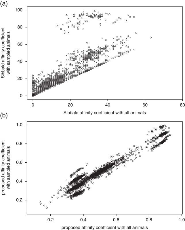
When only 8 of the 12 animals were observed in each simulation, affinities within pairs based on the Sibbald index were strongly biased for recently mixed and family groups (Figure 4a). Circles were gathered around (8, 14), whereas diamonds were spread in a stripe above the first diagonal. Triangles and crosses were also spread in this stripe, with some of them gathered around (32, 95) for triangles and (29, 87) for crosses, and some pairs reaching extreme values with an estimation equal to 100 (i.e. these animals were always recorded as nearest neighbours). Pairs in groups where interactions were fitted with a lognormal distribution (diamonds) showed all intermediate values, depending on the sampling effect and on affinities. Conversely, estimates based on the proposed index did not show such a bias (Figure 4b), even if estimate values were affected by the strength of affinity relationships of missing animals. Circles were gathered around (0.5, 0.5) in an ellipse spread along the first axis and diamonds were also spread along the first axis. Triangles and crosses were split into two groups centred around (0.36, 0.37) and (0.9, 0.9) for triangles (recently mixed groups), and (0.37, 0.37) and (0.87, 0.87) for crosses (family groups), which corresponds to unbiased estimation of the two kinds of affinities.
Comparison between the affinity coefficients between 2 animals when 8 randomly chosen animals of the 12 were observed and when all animals were observed using the Sibbald index (a) or the proposed index (b). Circles: groups of independent animals; triangles: recently mixed groups; crosses: family groups; diamond: continuously distributed affinities.

In conclusion, the two procedures aiming to quantify the variability in affinity relationships in a group of domestic herbivores led to correlated but not equal estimators. The proposed index was more robust to missing data, especially when affinities within pairs of animals were considered.
Characteristics of the proposed index
Figure 5 shows how the statistical properties of
 $\hat{U}_{g} $
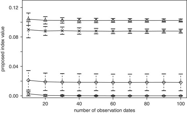
, the estimator of the global variance of affinities, vary according to the number of observation dates and group structure in groups of 15 animals (3 subgroups of 5 animals in recently mixed and family groups). The mean value of estimator
 $\hat{U}_{g} $
of the global variance of affinities in the group was highly stable. The standard deviation calculated on the 100 simulations was the smallest for groups of independent animals, and the largest in groups where interactions were fitted with a lognormal distribution.
Evolution of U g , the variance of the affinity coefficients according to the number of observation dates on groups of 15 animals. Circles: groups of independent animals; triangles: recently mixed groups; crosses: family groups; diamond: continuously distributed affinities; plain lines: mean values of the biased estimator; vertical bars: ±the standard deviation.

Figure 6a shows how
 $\hat{U}_{g} $
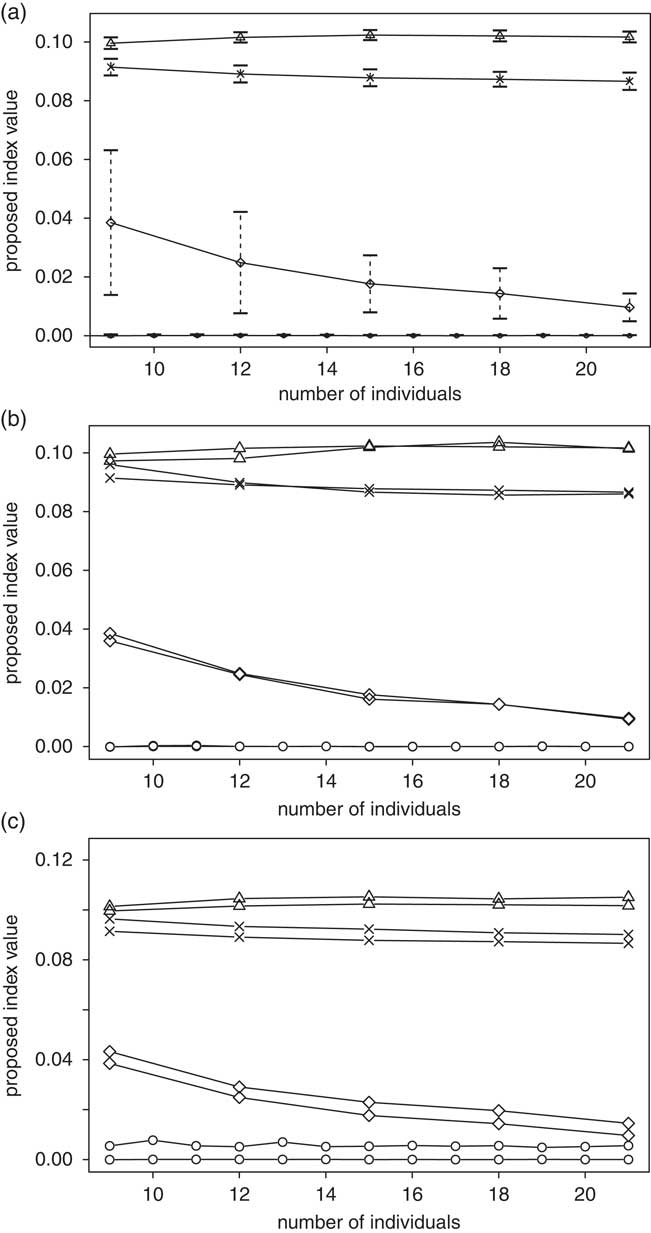
varies with the number of individuals inside the group. We simulated groups of independent animals varying from 3 to 21 individuals; recently mixed and family groups were made of 3 subgroups of 3 to 7 animals. The number of animals in groups where interactions were fitted with a lognormal distribution was 9, 12, 15, 18 or 21.
Effect of the group size on the variance of the affinity coefficients U g with 30 observations dates when (a) all animals are observed (b) the same animals are always observed at each date, (c) animals are randomly chosen at each date (line thickness is proportional to the sampled ratio). Circles: groups of independent animals; triangles: recently mixed groups; crosses: family groups; diamond: continuously distributed affinities; plain lines: mean values of the biased estimator; vertical bars: ±the standard deviation.

Variability in affinity relationships depended on group structure: they were low, independent of group size and with small variations in groups of independent animals. They were also stable for recently mixed or family groups larger than 12 animals. Conversely, they sharply decreased in groups where interactions were fitted with a lognormal distribution. In this case, the larger the group, the more interactions were sampled, and therefore the more individuals with similar interactions for each focus animal. For the lognormal group structure, variability of
 $\hat{U}_{g} $
was also greater than for the other group structures, and decreased as group size increased.
We then considered that only a sub-sample of the animals could be observed in each of the simulated data sets used above. We made the sample ratio being either 0 (all individuals are sampled), 0.1, 0.3 or 0.6 and analysed the behaviour of
 $U_{g} $
according to the number of individuals in the group. Two sampling procedures were considered. In Figure 6b, the same subset of animals for a given simulation did not vary across measurement days. In Figure 6c, the missing animals were randomly sampled at each date. When the same animals were observed across measurement days, all mean value curves for a given group structure were close to each other (Figure 6b), and variances decreased with the number of sampled animals as expected. Mean value curves presented the same pattern when missing animals changed across dates in Figure 6c.
Real case study
We recorded the daily paths and animal distribution during active grazing periods using GPS telemetry collars with differential correction (Schlecht et al., Reference Schlecht, Hülsebusch, Mahler and Becker2004) across different experiments involving groups of heifers of the same age, with no family ties (i.e. no twins) ranging from 3 to 27 animals (Dumont et al., Reference Dumont, Garel, Ginane, Decuq, Farruggia, Pradel, Rigolot and Petit2007; Della-Rossa et al., Reference Della-Rossa, Chadœuf, Boissy and Dumont2013; Dumont, unpublished data). Heifers were continuously grazing in semi-natural upland pastures, with 2 or 3 days of measurement per group that were spread along the grazing season. Frequency of random breakdown of GPS collars is reported in Table 1. In groups of nine animals, either seven or nine animals were equipped according to the experiments. In groups of 27 animals, only the same 10 animals of each group were equipped. Grazing activity was defined based on the ‘head-down’ position of Ethosys collars (Scheibe et al., Reference Scheibe, Schleusner, Berger, Eichhorn, Langbein, Dal Zotto and Streich1998), and our estimator was computed when at least two-thirds of the recorded animals were grazing. Recording periods were then sub-sampled for 5 min each to match the sampling interval chosen by Sibbald et al. (Reference Sibbald, Elston, Smith and Erhard2005). All the recordings for a given group were then merged as affinities are stable in familiar cattle herds (Bouissou et al., Reference Bouissou, Boissy, Le Neindre and Veissier2001; Gygax et al., Reference Gygax, Neisen and Wechler2010).
Characteristics of the observed data sets, global variance
 $\hat{U}_{g} $
and significativity of the test of affinity equality

GPS=global positioning system.
First, we tested whether affinities were equally spread in each group using a randomization test with 1000 independent simulations. We therefore randomly reallocated animal identity in each group date by date, before computing the estimator in the same way as for original data. The assumption that inter-individual affinities are equal was rejected if the estimator value of original data was out of the range of 0.95 of the simulations. The test of equal affinity inside a group was strongly rejected (P-value<0.05), except for 5 groups (out of 15) of 3 animals, although animals were of the same age and with no family ties.
Second, under the assumption that groups of a given size are independent replicates, we estimated the evolution of the affinity index (respectively, its precision) according to group size as the mean (respectively, the variance) of the index values of groups of a given size. We then tested whether affinities between members of groups of a given size were equal by computing 1000 mean index values over the same number of observations in groups of the same size under the equality assumption. We then computed a 95% confidence band of the mean over observed data for each size. Table 1 shows how
 $\hat{U}_{g} $
, the estimator of the variance of the affinity, changes according to group size. Variability in affinity relationships was the greatest in groups of five and seven animals, and it was lower for either smaller or larger groups. The estimator dispersion, measured through its standard deviation, is also given in Table 1. Effect of group size can be discussed as follows.
In very small groups (three animals), an animal may or may not find another animal with which it develops strong affinity relationships. This led to a highly variable index, with a low mean (Table 1) as the equal affinity hypothesis could not be rejected for one-third of the groups. This could also suggest that animals grazing in very small groups may not behave in the same way as in larger groups (Penning et al., Reference Penning, Parsons, Newman, Orr and Harvey1993). Consistently, calves that were reared in small groups lied down and expressed allogrooming indifferently towards familiar or unfamiliar peers after regrouping, whereas in larger groups grooming interactions were not uniformly distributed among group members (Færevik et al., Reference Færevik, Andersen, Jensen and Bøe2007).
As group size increases (five and seven animals), the probability of having constituted a group in which each animal developed strong affinities with at least another animal also increased, so that the average value of
 $U_{g} $
, the variance affinity, was the highest. For animals kept indoors, where the surface available for each animal is reduced, there could be an additive effect of dominance relationships. Staying close to a socially bonded peer may then reduce the expression of agonistic interactions owing to a greater tolerance between animals as it has been shown in cattle (Bouissou et al., Reference Bouissou, Boissy, Le Neindre and Veissier2001).
As group size further increases, the probability for each animal to have several peers with which to develop similar affinities also increases. Consistent to what was evidenced in groups where social interactions were fitted with a lognormal distribution (see ‘Simulation study’ section), triplets with animals of similar affinity have a low contribution to the index so that the average value of estimator U g decreased. In our data set, this phenomenon already occurred in groups of nine heifers.
In the largest groups, we could have expected the formation of subgroups as an increase in the group size can result in a decrease in social interactions (Sueur et al., Reference Sueur, Deneubourg, Petit and Couzin2011) when consensus costs outweigh the benefits of group cohesion for some individuals (see also King et al., Reference King, Douglas, Huchard, Isaac and Cowlishaw2008; Conradt and Roper, Reference Conradt and Roper2010). The low value of affinity variance estimator U g suggests that either the large groups rarely split into subgroups, or that the composition of these subgroups could be variable in grazing heifers.
Conclusion
Our method allows analysing the variability in affinity relationships in partially observed groups of domestic herbivores. It is based on the estimation of the probability that any random animal is closer to a focus animal than another animal of its group, which extends the basic idea of Sibbald et al. (Reference Sibbald, Elston, Smith and Erhard2005) without requiring the whole group to be observed at each measurement date. If missing data are randomly distributed among animals of a given group at each date, it provides an unbiased estimator of affinity variability inside the group, as all triplets will be observed as the number of observation dates increases. Moreover, classic methods such as bootstrapping of dates could give access to the variance of the estimators even if all animals are never simultaneously observed (Efron and Tibshirani, Reference Efron and Tibshirani1993).
If the same animals are equipped at all observation dates (equipped animals being chosen randomly), the estimator of affinity variability becomes biased; however, it remains unbiased at the population level, that is, if several independent groups are being analysed. Variance of affinity estimators at the level of the triplets are always accessible for observed triplets of animals, but the variance of the global affinity estimator of a given group cannot be estimated, as no data are available for animals that were not equipped. Independent group replicates can, however, be used to estimate variability in affinity relationships at the population level, as a classic variance analysis of indices computed on the independent groups will give unbiased estimators at the population level.
The proposed index allows comparing affinity variability on groups of different size, as its mean value is independent of the number of animals in the group contrarily to previously developed methods based on the frequency that any animal is recorded as the nearest animal of the focus animal. In the real case study, we showed that even in homogeneous groups of heifers variability in affinity relationships led to the development of strong group structures. The test of equal affinity inside a group was indeed always rejected, except for one-third of the groups of three animals. Our observations suggest that variability in affinity relationships would be the highest in groups of intermediate sizes.
Automatic recording of animal distribution was thus successful for identifying and summarizing the structure of group affinities. Several authors have attempted to detect and identify collective phenomena within movement data (Laube et al., Reference Laube, Kreveld and Imfeld2005; Andersson et al., Reference Andersson, Gudmundsson, Laube and Wolle2007; Miller and Gerlai, Reference Miller and Gerlai2011; Wood, Reference Wood2011). Coupling affinity structure and collective movement recordings based on measurements obtained with the same telemetry collars would make it possible to model collective decisions and grazing distribution in domestic herbivores.
Acknowledgements
Lia Della-Rossa was funded by a grant provided by INRA Phase division. We are grateful to Alain Boissy for helpful comments on an early version of the manuscript.