1 Introduction
Biologists and engineers alike have long been captivated by the grace and fluidity of fish and other undulatory swimmers. These animals achieve locomotion by generating a backwards propagating wave along their body which interacts with the surrounding fluid to generate a propulsive force. Over the past century the relationships between body wave kinematics, animal physiology, and propulsive performance have been studied from a wide variety of perspectives, ranging from neurology and muscle dynamics to systems control and fluid mechanics. Throughout these fields, particular interest has been devoted to the problem of optimally efficient locomotion. From a biological perspective, efficiency is potentially a strong motivator of behaviour and physiology. From an engineering perspective, it is hoped that the endurance of natural swimmers can be emulated in the design of aquatic vehicles. Within the following study we explore the physics of efficient undulatory propulsion for slender animals swimming at high Reynolds number,
 $Re=V\ell /\unicode[STIX]{x1D708}$
, where
 $V$
is swimming velocity,
 $\ell$
is body length, and
 $\unicode[STIX]{x1D708}$
is the kinematic viscosity of the surrounding fluid.
We begin with a brief review of high-
 $Re$
swimming, from the works of Lighthill up to the present day. While earlier studies such as those of Gray (Reference Gray1936) and Taylor (Reference Taylor1952) represent valuable contributions, Lighthill’s work is the first to properly capture the inertial effects which propel high-
 $Re$
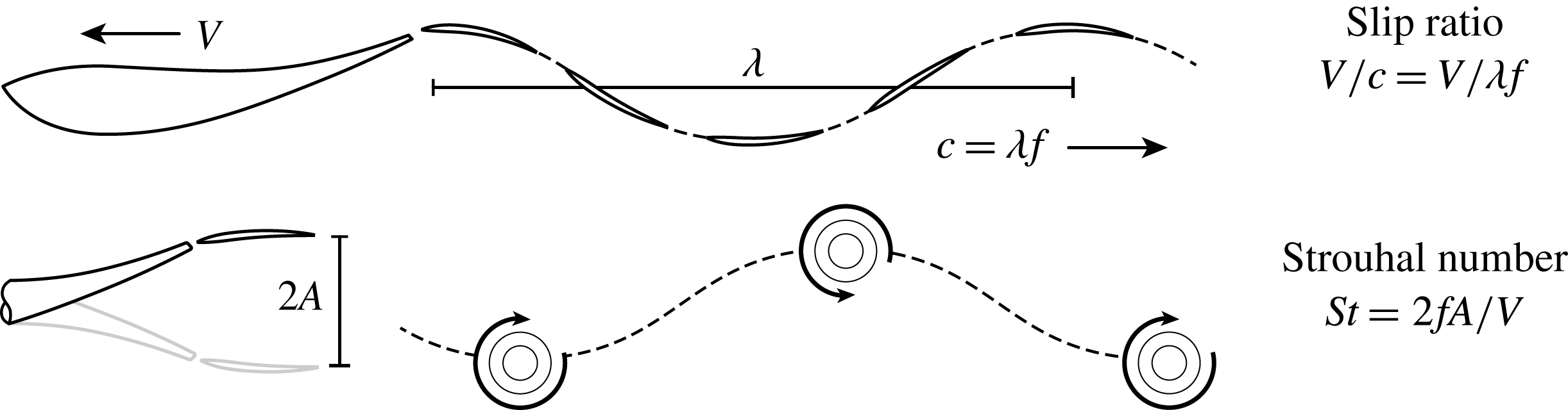
swimmers. The core of Lighthill’s contribution consists of his elongated-body theory of fish locomotion. Drawing upon analytical methods for the study of slender bodies such as airships, he constructs a compact model of swimming physics in the inertial regime. Under the assumption of small-amplitude swimming motions Lighthill (Reference Lighthill1960) demonstrates that swimming efficiency is determined by a single variable: the slip ratio (
 $V/c$
). The slip ratio quantifies swimming velocity (
 $V$
) relative to the backwards propagation speed
 $c$
of the body wave, as shown in figure 1, where
 $f$
is tailbeat frequency and
 $\unicode[STIX]{x1D706}$
is the wavelength of undulation. Lighthill found that as the slip ratio approaches one, efficiency rises to 100 % while thrust drops to zero. To minimize power consumption during locomotion, he concludes that animals must attempt to maximize
 $V/c$
while maintaining enough thrust to overcome drag. The simplicity of this result is appealing; however, its applicability is limited by the small-amplitude restriction. Expanding on his previous work, Lighthill (Reference Lighthill1971) develops a large-amplitude version of elongated-body theory in which the performance of the swimmer is a function of both the slip ratio and the Strouhal number
 $(St)$
. This large-amplitude version of Lighthill’s theory forms the core of the analysis presented here.
Definitions of the slip ratio and Strouhal number for undulatory swimming.

Twenty years after Lighthill’s work, a shift in focus was brought about by the findings of Triantafyllou, Triantafyllou & Gopalkrishnan (Reference Triantafyllou, Triantafyllou and Gopalkrishnan1991). Triantafyllou observed a consistent wake morphology among swimming species with foil-like tails. During undulation, a vortex is shed at each reversal of the tail beat. This produces a series of counter-rotating vortices behind the animal, as shown in figure 1. In dimensionless terms, bluff body wakes are classically described using the Strouhal number,
 $St_{b}=fd/V$
, where
 $f$
is the frequency of vortex shedding,
 $d$
is the diameter of the body, and
 $V$
is flow velocity. Triantafyllou adapts
 $St$
to describe the swimming wake by replacing body diameter with the amplitude of the tail beat,
 $St=2fA/V$
. In this form,
 $St$
provides a simple but direct connection between the kinematics of a swimming animal and its trailing wake (Triantafyllou, Triantafyllou & Yue Reference Triantafyllou, Triantafyllou and Yue2000). Triantafyllou et al. (Reference Triantafyllou, Triantafyllou and Gopalkrishnan1991) observed that swimming animals with foil-like tails adhere to a relatively narrow
 $St$
range,
 $0.2<St<0.4$
. Through experiments he then showed that the efficiency of an isolated flapping foil peaks at a similar value.
Many studies have since confirmed the observations of Triantafyllou; examples include the compiled datasets of Taylor, Nudds & Thomas (Reference Taylor, Nudds and Thomas2003) and Rohr (Reference Rohr2004). Although the significance of
 $St$
is well established, the physical basis for the observed optimal range is still a topic of debate. Triantafyllou, Triantafyllou & Grosenbaugh (Reference Triantafyllou, Triantafyllou and Grosenbaugh1993) propose that it is determined by the convective instability of the wake. During swimming, a shear flow profile is produced immediately behind the trailing edge of the tail – the unstable nature of this flow profile causes it to evolve into a vortex wake as it propagates away from the animal. Triantafyllou et al. (Reference Triantafyllou, Triantafyllou and Grosenbaugh1993) explain that the unstable wake acts as a tuned amplifier which magnifies the animal’s perturbing tailbeat. Based on this, they suggest that swimming animals tune their motions to strengthen the efficient vortex wake by matching their kinematics to the resonant frequency of the wake dynamics. In recent work, Moored et al. (Reference Moored, Dewey, Smits and Haj-Hariri2012, Reference Moored, Dewey, Boschitsch, Smits and Haj-Hariri2014) test this hypothesis using experimental flow profiles produced by a flapping mechanical fin (Clark & Smits Reference Clark and Smits2006). Moored et al. (Reference Moored, Dewey, Smits and Haj-Hariri2012, Reference Moored, Dewey, Boschitsch, Smits and Haj-Hariri2014) demonstrate that resonance conditions often do correspond to local peaks in efficiency. Based on these results, it is clear that wake resonance can influence the performance of flapping foils; further work is required to understand how these effects transfer to elongated animals.
Linden & Turner (Reference Linden and Turner2004) propose an alternative explanation for the
 $St$
range of undulatory swimmers. Based on an analysis of vortex ring formation (Linden & Turner Reference Linden and Turner2001), they suggest that swimming efficiency is not a function of bulk wake structure. Instead, it is proposed that thrust generation and power consumption are determined by the isolated properties of individual vortex rings within the wake. Linden and Turner hypothesize that swimming kinematics are chosen to produce optimal vortex rings which maximize their momentum while minimizing total kinetic energy. Dabiri (Reference Dabiri2009) discusses this hypothesis extensively in the context of jet-based propulsion as employed by squid and jellyfish, but a rigorous investigation of undulatory swimming has yet to be conducted from this perspective.
Triantafyllou’s experiments use high-aspect-ratio flapping to foils to approximate the tails of scombrid fish such as tuna and mackerel or cetaceans such as dolphins and whales. These animals are among nature’s fastest and most efficient swimmers, but they represent just a fraction of the full range of swimming species within the natural world. The analysis presented here considers swimming animals with slender elongated-body shapes that cannot be approximated as foils. Examples include salmonid fish such as trout and salmon or anguillids such as the American and European eel. The kinematics of elongated animals often deviate from the 0.2–0.4
 $St$
range and studies have shown that they produce a variety of complex wake morphologies which differ from the singular counter-rotating vortices of foil-tail swimmers (Muller et al.
Reference Muller, Smit, Stamhuis and Videler2001; Tytell et al.
Reference Tytell, Borazjani, Sotiropoulos, Baker, Anderson and Lauder2010; Eloy Reference Eloy2012).
In an effort to understand the behaviour of these animals, a wide range of hydrodynamic models have been used to explore the complex relationship between kinematics, efficiency, and swimmer geometry. In their full form, these relationships are governed by a three-dimensional interaction between the swimmer’s body and the surrounding fluid. A number of studies have applied computational methods to directly simulate this three-dimensional system. Examples include the work of Kern & Koumoutsakos (Reference Kern and Koumoutsakos2006), which applies evolutionary optimization methods to identify efficient and high-velocity swimming motions for a three-dimensional anguilliform swimmer; van Rees, Gazzola & Koumoutsakos (Reference van Rees, Gazzola and Koumoutsakos2013), which applies a similar approach to study optimal body shapes with imposed kinematics; van Rees, Gazzola & Koumoutsakos (Reference van Rees, Gazzola and Koumoutsakos2015), which considers optimal body shape and kinematics simultaneously; and the work of Maertens, Gao & Triantafyllou (Reference Maertens, Gao and Triantafyllou2017), which considers optimal kinematics and fish schooling interactions.
A number of studies have also applied reduced order models to study swimming systems. Although this approach cannot provide the detailed flow visualizations of full computational methods, the transparency of these simplified models has produced a number of significant insights. Gazzola, Argentina & Mahadevan (Reference Gazzola, Argentina and Mahadevan2014) constructs a simple scaling argument to explain why the kinematics of intermediate-
 $Re$
swimmers differ from those at high
 $Re$
, Tokić & Yue (Reference Tokić and Yue2012) apply Lighthill’s elongated-body theory in combination with numerical optimization to accurately predict form and behaviour for a range of different swimming species, and Eloy (Reference Eloy2012, Reference Eloy2013) uses a similar approach to demonstrate that optimal
 $St$
varies systematically with the body drag and tail size of swimming animals.
Here, we build upon the findings of Eloy (Reference Eloy2012). Using Lighthill’s large-amplitude elongated-body theory, we show that optimally efficient swimming kinematics can be reduced to a single dimensionless variable,
 $\unicode[STIX]{x1D713}$
, which is defined by a simple function of a swimming animal’s body wave properties. This variable,
 $\unicode[STIX]{x1D713}$
, characterizes how the velocity of the animal’s tail varies in time as it beats back and forth through the surrounding fluid. Using Lighthill’s model, we show that regardless of a swimming animal’s size and shape, peak efficiency is always achieved at
 $\unicode[STIX]{x1D713}=0.87$
. At this point, the average magnitude of the tail velocity is minimized and the animal produces a relatively constant thrust coefficient throughout its swimming stroke. We use a compiled dataset of over 250 unique measurements of swimming animals to show that species across a wide range of size and shape follow the predicted optimum.
The current understanding of efficient swimming at high
 $Re$
is founded upon Triantafyllou’s pioneering work on vortex shedding and flapping foils. Triantafyllou demonstrated that lunate tail swimmers adhere to a narrow optimal
 $St$
range of 0.2–0.4, where they produce a characteristic vortex wake. Biological measurements have since confirmed that
 $St$
plays a critical role in the behaviour of swimming animals across a wide range of morphologies, but it is currently unclear how Triantafyllou’s results translate to slender animals with elongated tails. Within Lighthill’s model, we find that optimality is entirely determined by the variable
 $\unicode[STIX]{x1D713}$
;
 $St$
is instead determined by thrust–drag balance. While
 $\unicode[STIX]{x1D713}=0.87$
characterizes the optimal undulation pattern for efficient swimming,
 $St$
scales the magnitude of this pattern, such that the thrust output of the tail can be adjusted to match the drag of the body.
2 Constructing the swimming model
We begin by establishing the details of the swimming model applied throughout our analysis. The model description is divided into three subsections: (1) geometry and kinematics, (2) Lighthill’s large-amplitude elongated-body theory, and (3) thrust and power consumption during steady swimming.
2.1 Geometry and kinematics
Throughout our analysis we refer to slender swimmers as being distinct from foil-tailed animals. Slender swimmers are characterized by a low aspect ratio,
 $AR=h/L$
, and slowly varying cross-sectional shape, where
 $h$
is the height of the trailing edge and
 $L$
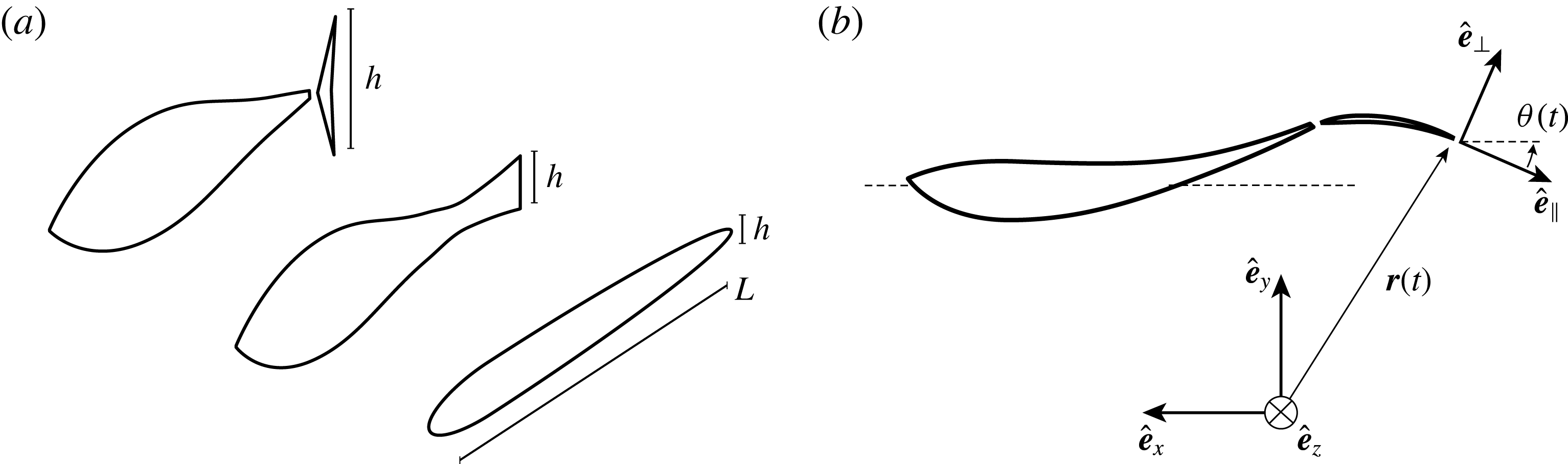
is body length. In figure 2, we compare the body forms of an eel-, a trout-, and a tuna-like swimmer. Since Lighthill’s model assumes a slender geometry, our analysis is applicable to animals with shapes similar to the eel and trout, but not the tuna, which exhibits a distinct foil-like tail.
(a) Comparison of slenderness (
 $h/L$
) for tuna-, trout-, and eel-type swimmers. (b) Coordinate frames and functions used to describe the motion of the swimmer.

Within Lighthill’s elongated-body theory, the thrust and power consumption of a swimming animal are fully determined through the motion of its trailing edge. To define the kinematics at this point, we apply the definition of Eloy (Reference Eloy2012). The swimmer is assumed to travel forward at a constant velocity
 $V$
and the trailing edge is prescribed to undergo periodic heaving and pitching with a phase lag of
 $\unicode[STIX]{x03C0}$
between the two motions. This approximates the wave-like tail motion of natural swimmers as shown in figure 1 (Lighthill Reference Lighthill1969). The resulting kinematics are defined through the position
 $\boldsymbol{r}(t)$
and angle
 $\unicode[STIX]{x1D703}(t)$
of the tail, shown in figure 2 and given as
 $$\begin{eqnarray}\boldsymbol{r}(t)=Vt\hat{\boldsymbol{e}}_{x}+A\cos (2\unicode[STIX]{x03C0}ft)\hat{\boldsymbol{e}}_{y}\quad \text{and}\quad \unicode[STIX]{x1D703}(t)=\unicode[STIX]{x1D6FD}\sin (2\unicode[STIX]{x03C0}ft).\end{eqnarray}$$
These kinematics are characterized by four parameters: frequency (
 $f$
), amplitude (
 $A$
), pitching angle (
 $\unicode[STIX]{x1D6FD}$
), and velocity
 $(V)$
. These parameters reduce to two dimensionless groups, pitch angle
 $\unicode[STIX]{x1D6FD}$
and the Strouhal number
 $St=2fA/V$
. If we assume the path of the tail approximates a sinusoidal wave, pitch angle can be related to Lighthill’s slip ratio as follows (see appendix A for a derivation of this relation):
 $$\begin{eqnarray}\unicode[STIX]{x1D6FD}=\unicode[STIX]{x03C0}\frac{V}{c}St.\end{eqnarray}$$
Here, we often use the slip ratio,
 $V/c$
, in place of
 $\unicode[STIX]{x1D6FD}$
, as
 $V/c$
is widely used in previous studies.
To quantify the thrust and power consumption of the swimmer we need to determine the tangential and normal components of the trailing edge velocity. They can be calculated by taking the time derivative of the position vector,
 $\boldsymbol{r}$
, and projecting the result on to
 $\hat{\boldsymbol{e}}_{\bot }$
and
 $\hat{\boldsymbol{e}}_{\Vert }$
as follows:
 $$\begin{eqnarray}v_{\bot }=\frac{\text{d}\boldsymbol{r}}{\text{d}t}\boldsymbol{\cdot }\hat{\boldsymbol{e}}_{\bot }\quad \text{and}\quad v_{\Vert }=\frac{\text{d}\boldsymbol{r}}{\text{d}t}\boldsymbol{\cdot }\hat{\boldsymbol{e}}_{\Vert }.\end{eqnarray}$$
We then non-dimensionalize
 $v_{\bot }$
and
 $v_{\Vert }$
against the swimming velocity
 $V$
and normalize time against the swimming frequency. This produces the following expressions:
 $$\begin{eqnarray}\displaystyle & \displaystyle v_{\bot }^{\ast }=\frac{v_{\bot }}{V}=-\unicode[STIX]{x03C0}St\cos (\unicode[STIX]{x1D6FD}\sin (t^{\ast }))\sin (t^{\ast })+\sin (\unicode[STIX]{x1D6FD}\sin (t^{\ast })), & \displaystyle\end{eqnarray}$$
 $$\begin{eqnarray}\displaystyle & \displaystyle v_{\Vert }^{\ast }=\frac{v_{\Vert }}{V}=-\unicode[STIX]{x03C0}St\sin (\unicode[STIX]{x1D6FD}\sin (t^{\ast }))\sin (t^{\ast })-\cos (\unicode[STIX]{x1D6FD}\sin (t^{\ast })), & \displaystyle\end{eqnarray}$$
where
 $t^{\ast }=2\unicode[STIX]{x03C0}ft$
.
2.2 Fluid forces
Within Lighthill’s large-amplitude elongated-body theory (Lighthill Reference Lighthill1971), the thrust produced by a swimmer (
 $\overline{T}$
) is given by the streamwise projection of a normal force,
 $\boldsymbol{F}_{n}$
, and a tangential force,
 $\boldsymbol{F}_{t}$
. The normal force is produced by the inertial reaction of the fluid as the swimmer’s body undulates back and forth. The source of the tangential force is somewhat less intuitive. Lighthill (Reference Lighthill1971) demonstrates its existence through an energy balance, while Wu (Reference Wu1971) arrives at the same result by integrating over a leading edge singularity within the flow field around the swimmer’s tail. To calculate the average thrust generated over a complete a swimming cycle, we integrate the thrust over one full period, producing the following result, where
 $\unicode[STIX]{x1D70C}$
is fluid density. The notation used here is different from that of Lighthill (Reference Lighthill1971); the equivalency of our definitions is demonstrated in appendix C.
 $$\begin{eqnarray}\displaystyle & \displaystyle \overline{T}=f\int _{0}^{1/f}(\boldsymbol{F}_{n}(t)+\boldsymbol{F}_{t}(t))\boldsymbol{\cdot }\hat{\boldsymbol{e}}_{x}\,\text{d}t, & \displaystyle\end{eqnarray}$$
 $$\begin{eqnarray}\displaystyle & \displaystyle \boldsymbol{F}_{n}(t)=\frac{\unicode[STIX]{x03C0}}{4}\unicode[STIX]{x1D70C}V^{2}h^{2}\;(v_{\Vert }^{\ast }v_{\bot }^{\ast })\hat{\boldsymbol{e}}_{\bot }, & \displaystyle\end{eqnarray}$$
 $$\begin{eqnarray}\displaystyle & \displaystyle \boldsymbol{F}_{t}(t)=\frac{\unicode[STIX]{x03C0}}{4}\unicode[STIX]{x1D70C}V^{2}h^{2}\;\left(\frac{1}{2}v_{\bot }^{\ast 2}\right)\hat{\boldsymbol{e}}_{\Vert }. & \displaystyle\end{eqnarray}$$
The thrust integral of (2.6) is used to define a dimensionless thrust coefficient,
 $C_{T}(V/c,St)$
, given as
 $$\begin{eqnarray}\displaystyle & \displaystyle \overline{T}={\textstyle \frac{1}{2}}\unicode[STIX]{x1D70C}V^{2}h^{2}C_{T}, & \displaystyle\end{eqnarray}$$
 $$\begin{eqnarray}\displaystyle & \displaystyle C_{T}=\frac{1}{4}\int _{0}^{2\unicode[STIX]{x03C0}}\left(v_{\Vert }^{\ast }v_{\bot }^{\ast }\sin (\unicode[STIX]{x1D703}(t^{\ast }))+\frac{1}{2}v_{\bot }^{\ast \;2}\cos (\unicode[STIX]{x1D703}(t^{\ast }))\right)\text{d}t^{\ast }. & \displaystyle\end{eqnarray}$$
2.3 Thrust–drag balance during steady swimming
During constant-velocity swimming, the average thrust produced by the swimmer must be balanced by the drag of its body. This requirement is enforced by defining a drag force,
 $D$
, and setting
 $\overline{T}/D$
to be equal to one:
 $$\begin{eqnarray}\frac{\overline{T}}{D}=C_{T}\left(\frac{\frac{1}{2}\unicode[STIX]{x1D70C}V^{2}h^{2}}{D}\right)=1.\end{eqnarray}$$
The first term in this expression is the thrust coefficient. The second term, contained in parentheses, represents a ratio of the total drag on the fish and the thrust-generating capability of the tail. Following Eloy (Reference Eloy2012) we refer to this ratio as the Lighthill Number,
 $Li$
. Applying this definition reduces thrust–drag equilibrium to a simple dimensionless constraint:
 $$\begin{eqnarray}C_{T}=Li,\quad \text{where }Li=\frac{D}{\frac{1}{2}\unicode[STIX]{x1D70C}V^{2}h^{2}}.\end{eqnarray}$$
Physically,
 $Li$
represents the tail loading of the swimmer in a similar sense to the wing loading of a bird or insect. A swimming animal with a small
 $Li$
value would have a relatively large tail in relation to the drag of its body, while the tail of a high-
 $Li$
animal would be relatively small.
2.4 Power and efficiency
During swimming, energy generated by a swimmer’s muscles is dissipated through two distinct power sinks: useful thrust power, and kinetic energy left behind in the trailing wake. Following Lighthill, these can be quantified as
 $$\begin{eqnarray}P_{thrust}=\overline{T}V,\quad P_{wake}=-\frac{1}{8}\unicode[STIX]{x1D70C}V^{3}h^{2}\int _{0}^{2\unicode[STIX]{x03C0}}\left(\frac{1}{2}v_{\Vert }^{\ast }v_{\bot }^{\ast \;2}\right)\text{d}t^{\ast }.\end{eqnarray}$$
As proposed by Lighthill, we define the efficiency of the swimmer as a ratio of useful thrust power over the total power consumed by the animal:
 $$\begin{eqnarray}\unicode[STIX]{x1D702}=\frac{\overline{T}V}{\overline{T}V+P_{wake}}.\end{eqnarray}$$
If we non-dimensionalize both the numerator and denominator then divide through by
 $C_{T}V$
, efficiency reduces to the following, where
 $C_{P}$
is the dimensionless form of the wasted wake power (
 $P_{wake}$
):
 $$\begin{eqnarray}\unicode[STIX]{x1D702}=\frac{1}{1+C_{P}/C_{T}},\quad \text{where }C_{P}=-\frac{1}{4}\int _{0}^{2\unicode[STIX]{x03C0}}\left(\frac{1}{2}v_{\Vert }^{\ast }v_{\bot }^{\ast \;2}\right)\text{d}t^{\ast }.\end{eqnarray}$$
3 Optimally efficient swimming kinematics
At this stage we have fully defined and non-dimensionalized our swimming system. From (2.15), we see that the efficiency of the swimmer is solely determined through a ratio of the power and thrust coefficients
 $C_{P}/C_{T}$
. Using this result we can formally state the efficiency optimization problem as follows:
 $$\begin{eqnarray}\displaystyle & \displaystyle \underset{V/c,\,St}{\text{Minimize}}\quad C_{P}=-\frac{1}{4}\int _{0}^{2\unicode[STIX]{x03C0}}\frac{1}{2}v_{\Vert }^{\ast }v_{\bot }^{\ast \;2}\,\text{d}t^{\ast } & \displaystyle\end{eqnarray}$$
 $$\begin{eqnarray}\displaystyle & \displaystyle \text{subject to}\quad \frac{C_{T}}{Li}=\frac{1}{4}\int _{0}^{2\unicode[STIX]{x03C0}}\frac{(v_{\Vert }^{\ast }v_{\bot }^{\ast }\sin (\unicode[STIX]{x1D703}(t^{\ast }))+\frac{1}{2}v_{\bot }^{\ast \;2}\cos (\unicode[STIX]{x1D703}(t^{\ast })))}{Li}\,\text{d}t^{\ast }=1. & \displaystyle\end{eqnarray}$$
The resulting problem is equivalent to that of Eloy (Reference Eloy2012). In total, it contains three variables (
 $V/c$
,
 $St$
,
 $Li$
) and one constraint (
 $C_{T}=Li$
). Eloy (Reference Eloy2012) solves the problem numerically to determine the optimal relationship between the kinematic variables (
 $St$
,
 $V/c$
) and the tail loading
 $(Li)$
.
To assess the validity of the predicted relationships, Eloy (Reference Eloy2012) compares them to observed animal behaviour. He approximates the value of
 $Li$
for a given species by assuming that swimming drag arises predominantly through skin friction, such that
 $D=1/2\unicode[STIX]{x1D70C}C_{f}V^{2}S$
, where
 $C_{f}$
is a frictional drag coefficient and
 $S$
is the surface area of the animal. Through this comparison Eloy demonstrates that Lighthill’s model correctly predicts the
 $St-Li$
relationship of swimming animals. For
 $V/c$
and
 $Li$
the match is much weaker; this inconsistency can be attributed to the difficulties in determining accurate numerical values for
 $Li$
. Realistically, swimming drag (
 $D$
) is a complex function of shape, surface area and kinematics, and effects beyond skin friction may significantly contribute to its overall magnitude (Raspa et al.
Reference Raspa, Ramananarivo, Thiria and Godoy-Diana2014).
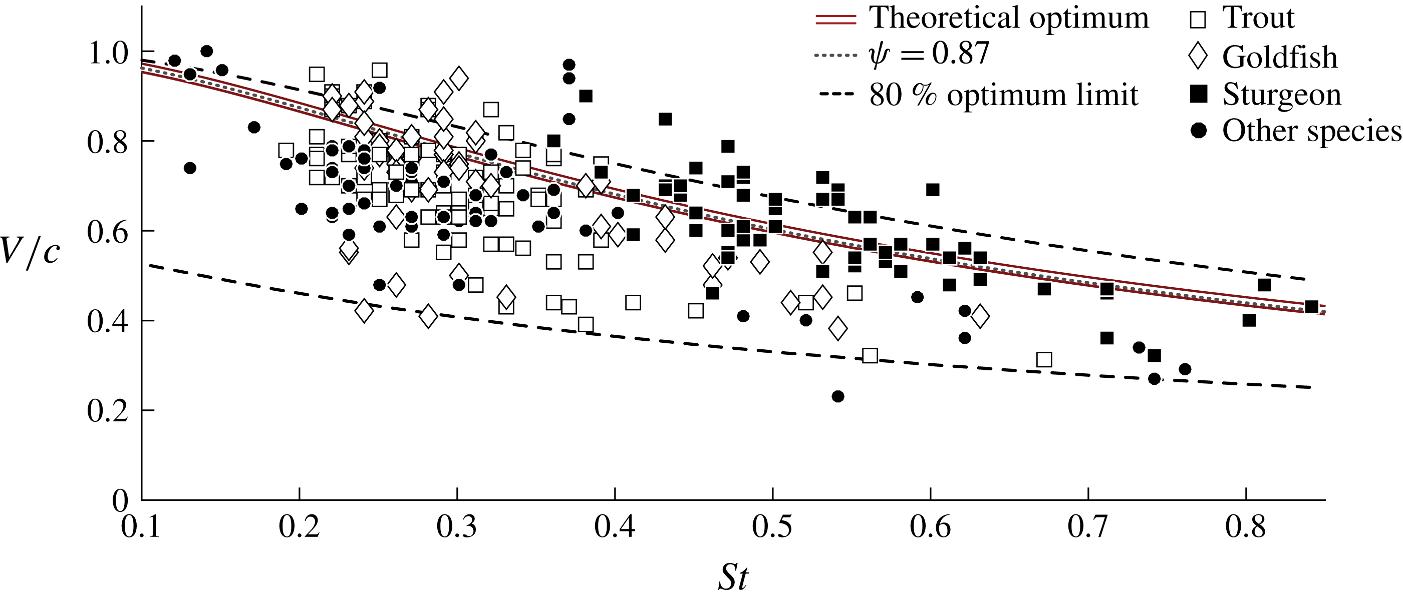
Comparison of optimal behaviour within Lighthill’s model and the observed
 $St$
and
 $V/c$
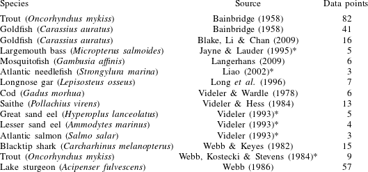
of natural swimmers. Dashed lines bracket the region where swimming efficiency is at least 80 % of its peak value for a given thrust coefficient. A list of the species within the dataset is provided in table 1. The raw dataset and further details on its contents are available online.

List of species within the compiled dataset. Data sources marked with a * are taken from the compilation of van Weerden, Reid & Hemelrijk (Reference van Weerden, Reid and Hemelrijk2014).

Here, we consider the solution as an optimal relationship between
 $St$
and
 $V/c$
. In this form, it can be compared to animal data without the need to approximate
 $Li$
. Assuming that a swimming animal must generate some finite amount of thrust, Lighthill’s model predicts that efficient swimmers should tune their kinematics to fall along the optimal
 $St-V/c$
curve. In figure 3 we plot this curve against a compiled dataset of over 250 unique observations of swimming kinematics for the 13 different animal species listed in table 1. Data points corresponding to trout, goldfish and sturgeon are highlighted with unique symbols as they constitute the bulk of the data. Through this comparison we see that the data points are distributed along the optimally efficient region, confirming Eloy’s finding that slender swimming animals do not always adhere to the 0.2–0.4
 $St$
range. Instead, it suggests that they adhere to an optimal
 $St-V/c$
relationship, with the exact position along this curve determined by the animal’s required thrust coefficient.
The raw dataset and further details on its contents are supplementary materials available online at https://doi.org/10.1017/jfm.2018.14. Constructing a meaningful dataset is a challenging process, as many if not most of the available studies on swimming kinematics are conducted using enclosed flow channels which can influence swimming behaviour and it can be difficult to determine whether swimming efficiency is a strong motivator for a given fish species. Nonetheless, considering the dataset as a whole, we see a clear trend along the predicted optimal region. Furthermore, the three species with the largest number of data points (trout, goldfish, and sturgeon) all exhibit swimming behaviours which fall outside the 0.2–0.4
 $St$
range, but sit along the optimal curve.
4 The physical basis of efficient swimming within Lighthill’s model
Having established that Lighthill’s model predicts both
 $St$
and
 $V/c$
for slender swimmers, in the following section we dissect this result to understand the physical effects which drive the optimal curve. Through this process we find that efficient swimmers tune their movements to minimize the average magnitude of
 $v_{\bot }$
and to produce an instantaneous thrust coefficient which varies as little as possible throughout the tailbeat.
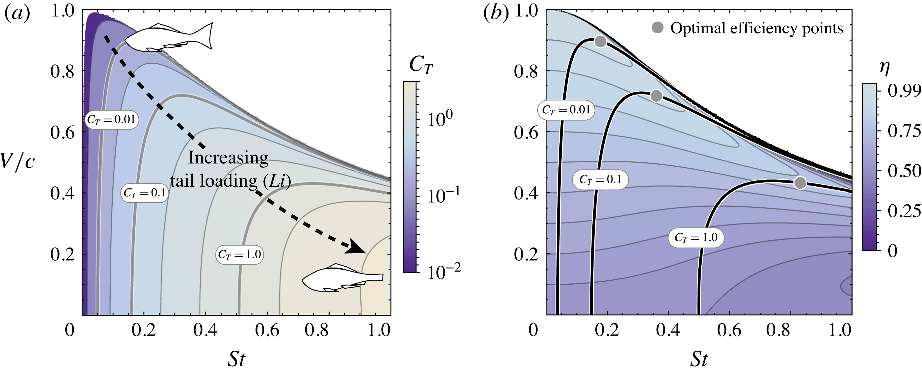
To show this, we begin by examining the underlying structure of the problem. In figure 4(a), the thrust coefficient,
 $C_{T}$
, is plotted over the
 $V/c{-}St$
plane. The thrust–drag constraint
 $(C_{T}=Li)$
is visualized through the resulting contours. An animal with tail size,
 $h$
, swimming with body drag
 $D$
has a fixed value of
 $Li$
. Consequently, it is constrained to use kinematics along the corresponding
 $C_{T}$
contour. From the plot we see that
 $C_{T}$
increases towards the bottom right corner, indicating that swimmers in this region must have small tails and large bodies, while the opposite is true in the upper left. Kinematics within the blank segment of the plot can be ignored as
 $C_{T}$
is negative within this region.
(a) Thrust coefficient plotted over a grid of slip and Strouhal values. A swimming animal with a given tail loading (
 $Li$
), is constrained to kinematics along a single level
 $C_{T}$
curve. (b) Froude efficiency plotted over the same grid. The overlaid curves illustrate the constraint between
 $V/c$
and
 $St$
during steady swimming.

In figure 4(b), we plot the efficiency of the swimmer over the same grid. The plot exhibits relatively horizontal bands, with efficiency tending towards a maximum as
 $V/c$
approaches 1. To demonstrate how
 $St$
impacts efficiency, we must consider the thrust–drag constraint
 $(C_{T}=Li)$
. Since an animal swimming with body drag
 $D$
is restricted to a single
 $C_{T}$
curve,
 $St$
and
 $V/c$
are not independent. Superimposing the constant thrust contours onto the efficiency plot, we see that efficiency is poor at the high and low
 $St$
limits of each curve, where slip converges to zero; between these two limits there is a narrow
 $St$
range where
 $V/c$
is maximized and efficiency is high. The animal data in figure 3 show that natural swimmers choose their kinematics to sit in this optimal region along the peaks of the constant thrust contours.
To get a sense of the physical effects which drive this structure we consider the form of the thrust and power coefficients. Within Lighthill’s model, swimming animals produce thrust through two distinct sources: a normal force from the acceleration of fluid mass (
 $\boldsymbol{F}_{n}$
) and a tangential force (
 $\boldsymbol{F}_{t}$
). In the vicinity of the optimum, the normal force dominates the efficient swimming problem (see appendix B). Based on this we examine a reduced thrust-to-power ratio:
 $$\begin{eqnarray}\frac{C_{T}}{C_{P}}\approx \frac{C_{n}}{C_{P}}=\frac{\displaystyle \int _{0}^{2\unicode[STIX]{x03C0}}v_{\Vert }^{\ast }v_{\bot }^{\ast }\sin (\unicode[STIX]{x1D703}(t^{\ast }))\,\text{d}t^{\ast }}{\displaystyle \int _{0}^{2\unicode[STIX]{x03C0}}-\frac{1}{2}v_{\Vert }^{\ast }v_{\bot }^{\ast 2}\,\text{d}t^{\ast }}.\end{eqnarray}$$
In this form the optimal swimming problem is dependent on three unique terms,
 $v_{\Vert }^{\ast }$
,
 $v_{\bot }^{\ast }$
, and
 $\sin (\unicode[STIX]{x1D703}(t^{\ast }))$
.
 $v_{\Vert }^{\ast }$
appears linearly in both the thrust and power integrals and thus has relatively little effect on overall swimming efficiency. Instead, the dominant role is played by
 $v_{\bot }^{\ast }$
. With
 $\boldsymbol{F}_{n}$
as the dominant thrust source, the constraint
 $(C_{T}=Li)$
scales linearly in
 $v_{\bot }^{\ast }$
, while the objective
 $(C_{P})$
scales quadratically. To gain insight into this problem form, we consider a similar system given as follows:
 $$\begin{eqnarray}\displaystyle & \displaystyle \underset{f(z)}{\text{Minimize}}\quad F_{cost}=\int _{0}^{1}f^{2}(z)\,\text{d}z & \displaystyle\end{eqnarray}$$
 $$\begin{eqnarray}\displaystyle & \displaystyle \text{subject to}\quad F_{output}=\int _{0}^{1}f(z)\,\text{d}z=G, & \displaystyle\end{eqnarray}$$
where
 $G$
is a constant and
 $f(z)$
is an arbitrary real function. If we substitute the trial solution
 $f(z)=G+\unicode[STIX]{x1D716}(z)$
, we find that
 $\unicode[STIX]{x1D716}(z)=0$
. In physical terms this means that any variation in the output of the system will tend to increase the overall cost of that output. Transferring this reasoning to our problem suggests that its form penalizes variations within
 $v_{\bot }^{\ast }$
. Efficiency optimization should favour kinematics which maintain a relatively constant thrust coefficient throughout the swimming motion.
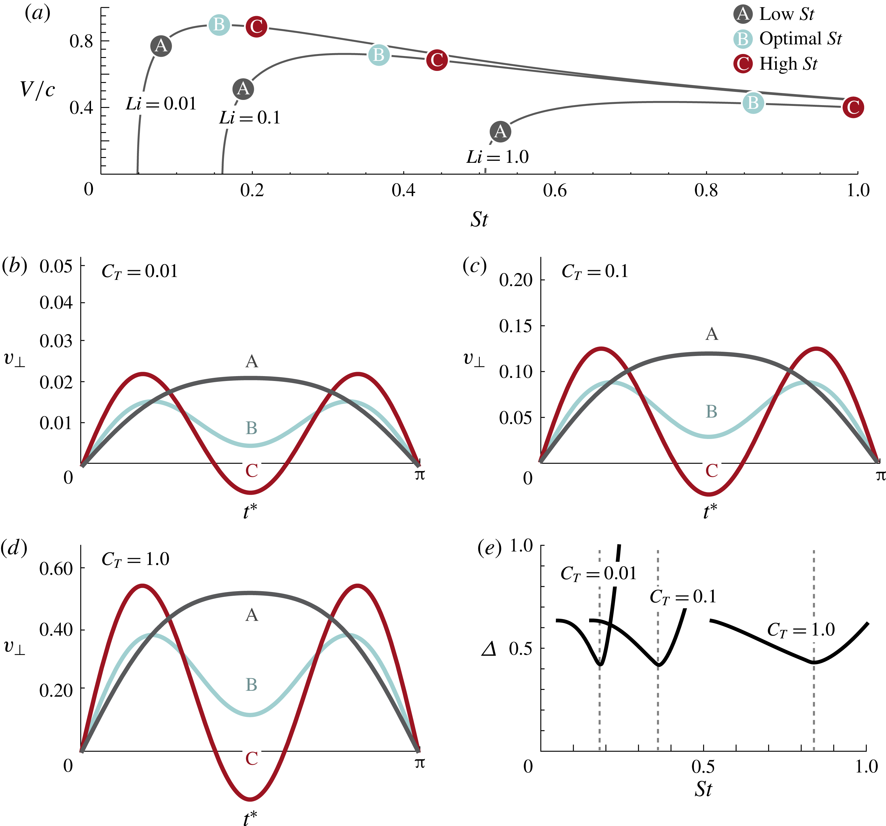
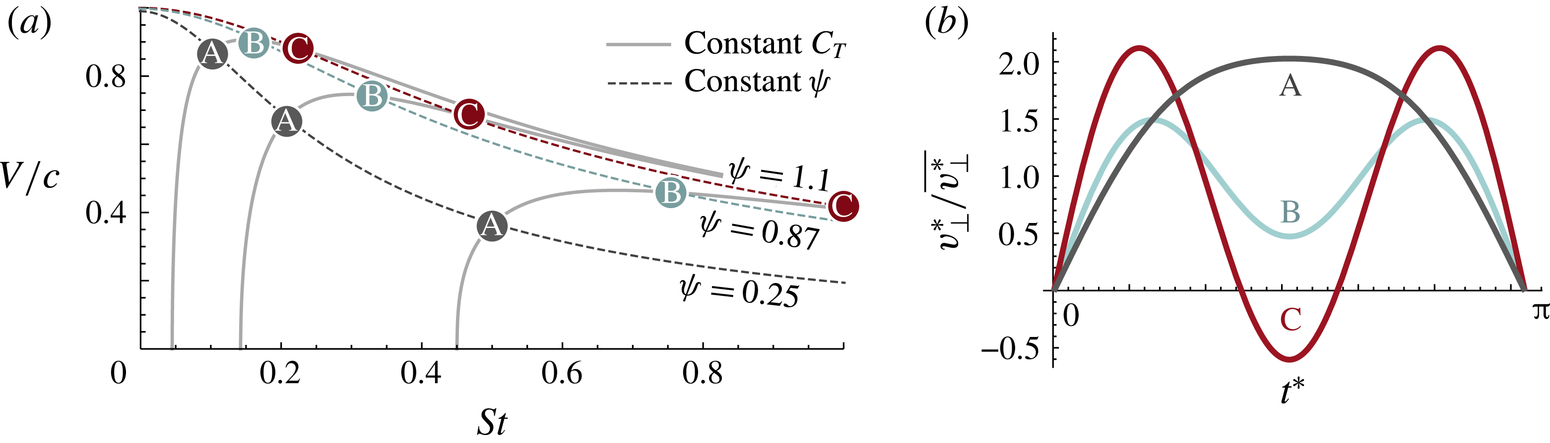
(a) Points are used to identify three distinct swimming regimes along the
 $C_{T}=0.01,\;0.1,\;1$
contours. (b–d) Comparison of
 $v_{\bot }^{\ast }$
profiles for each of the three swimming regimes. (e) Thrust coefficient variation,
 $\unicode[STIX]{x1D6E5}$
, plotted along constant thrust contours. Dashed lines mark points of maximum efficiency.

Based on this, swimming kinematics which generate strong peaks in
 $v_{\bot }^{\ast }$
should be inefficient, while those that yield a relatively flat
 $v_{\bot }^{\ast }$
profile should minimize energy consumption. We examine this relationship in figure 5(b–d), where
 $v_{\bot }$
profiles are plotted at three different points of the
 $C_{T}=0.01,0.1,1$
contours. Since the swimming motion is antisymmetric about
 $t^{\ast }=\unicode[STIX]{x03C0}$
, we show only the first half of the tailbeat cycle (
 $t^{\ast }=0-\unicode[STIX]{x03C0}$
). When
 $St$
is less than the optimal value, the profile exhibits a single large peak throughout each stroke of the tail. When
 $St$
is greater than the optimal value, a large negative trough appears in the centre of each stroke. The optimal
 $St$
value provides a balance between the two limits, producing a profile which oscillates near a mean constant value.
The steadiness of the thrust coefficient can be characterized by comparing its instantaneous value,
 $C_{T}^{i}$
, to its average value,
 $C_{T}$
. This is accomplished through the following metric,
 $\unicode[STIX]{x1D6E5}$
, which quantifies the mean variation in
 $C_{T}$
over each half of the tail beat:
 $$\begin{eqnarray}\unicode[STIX]{x1D6E5}=\frac{1}{\unicode[STIX]{x03C0}C_{T}}\int _{0}^{\unicode[STIX]{x03C0}}|C_{T}^{i}-C_{T}|\,\text{d}t^{\ast }.\end{eqnarray}$$
In figure 5(e),
 $\unicode[STIX]{x1D6E5}$
is plotted along the
 $C_{T}=$
0.01, 0.1, and 1 contours. The resulting curves show that the optimal stroke minimizes the variation of
 $C_{T}$
across all thrust levels.
Conceptually, the kinematics of the optimal solution are similar to the twisted design of a propeller blade. As a propeller rotates, blade sections at the outer radius move faster than those at the inner radius. To counter this effect, each blade is axially twisted such that pitch decreases towards the tip. This allows the propeller to maintain a constant angle of attack along its entire length (von Mises Reference von Mises1959). In the case of fish, the velocity of the tail tip varies in time rather than space, but kinematics are tuned to achieve a similar effect. The time-varying pitch of the tail balances changes in lateral velocity such that the thrust coefficient remains relatively constant throughout the full tail beat.
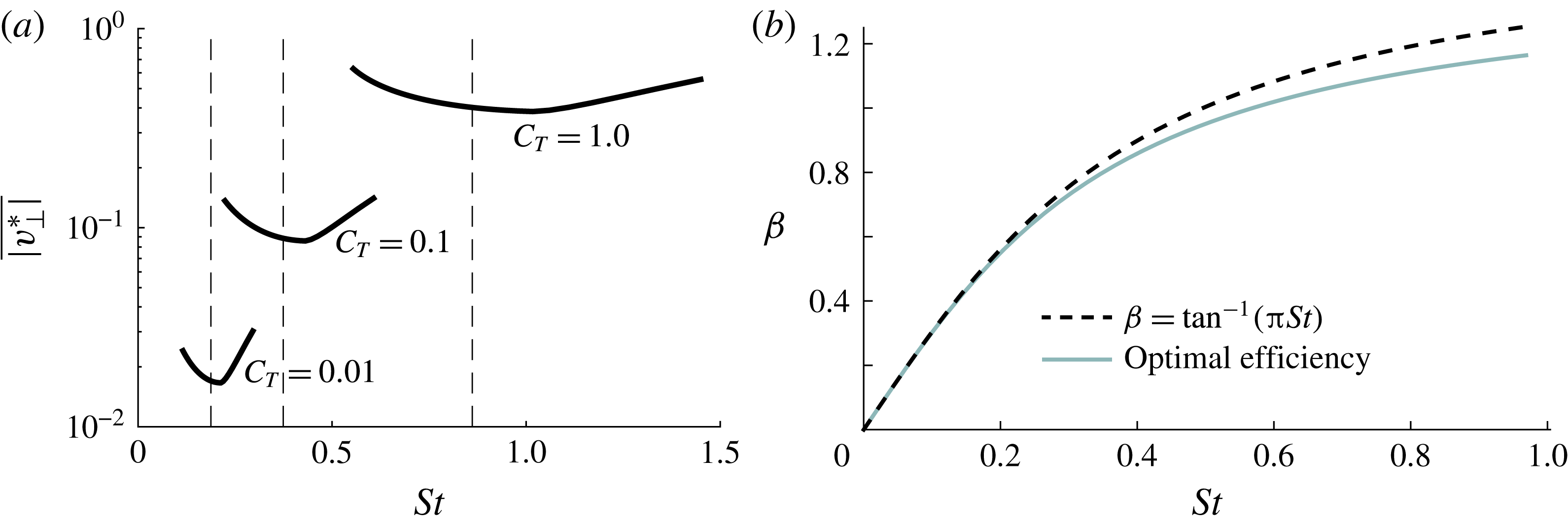
(a) Average magnitude of
 $|v_{\bot }^{\ast }|$
plotted along constant thrust contours. Dashed lines mark the point of optimal efficiency along each contour. (b) Comparison of the negative thrust threshold and the optimal efficiency curve in the
 $\unicode[STIX]{x1D6FD}{-}St$
plane.

In addition to minimizing variations in
 $C_{T}$
, kinematics along the optimal curve also tend to minimize the average magnitude of
 $v_{\bot }^{\ast }$
. We demonstrate this in figure 6(a), where we plot the average value of
 $v_{\bot }^{\ast }$
along the constant thrust contours. If we consider the form of the thrust output in (4.1), (
 $C_{T}=\int _{0}^{2\unicode[STIX]{x03C0}}v_{\Vert }^{\ast }v_{\bot }^{\ast }\sin (\unicode[STIX]{x1D703}(t^{\ast }))\,\text{d}t^{\ast }$
), we see that
 $v_{\bot }^{\ast }$
can be minimized by swimming with a large tail pitch,
 $\unicode[STIX]{x1D703}(t^{\ast })$
, to maximize the projected thrust component of the fluid momentum shed from the tail. However, if the pitch amplitude is too large,
 $v_{\bot }^{\ast }$
can become negative at the midpoint of the tailbeat. This can be observed in the high-
 $St$
profiles of figure 5. During periods where
 $v_{\bot }^{\ast }$
is less than zero, the swimmer produces negative thrust, effectively increasing the overall drag of its body and severely reducing swimming efficiency. The pitch amplitude associated with the onset of negative thrust production can be calculated by setting
 $v_{\bot }^{\ast }$
equal to 0 at
 $t^{\ast }=\unicode[STIX]{x03C0}/2$
. This produces the following relation:
 $$\begin{eqnarray}\unicode[STIX]{x1D6FD}=\tan ^{-1}(\unicode[STIX]{x03C0}St).\end{eqnarray}$$
In figure 6(b) we compare this relation to the efficiency optimum, in the
 $\unicode[STIX]{x1D6FD}{-}St$
plane. From the resulting curves we see that the optimum runs alongside the negative thrust limit. Swimming kinematics in this region maximize the projected thrust component while avoiding periods of negative thrust production.
4.1 Non-harmonic swimming motions
Taking the idea of minimal thrust variation to its limit, a swimming motion which produces perfectly constant thrust should provide the highest possible efficiency. Inspecting the form of our optimization problem, we can see that it supports this hypothesis. The integrands defining the thrust and power coefficients in (3.1) and (3.2) are purely dependent on the instantaneous state of the system. Based on this, it should be possible to maximize efficiency by identifying the tail angle and velocity which minimize power consumption on an instantaneous basis and then maintaining these values throughout each complete stroke of the tail. This motion can be produced by using square waves to define the lateral velocity,
 $\text{d}y/\text{d}t$
, and tail pitch,
 $\unicode[STIX]{x1D703}$
, such that the tail tip traces out a triangular path. In a sense, this result is the high-Reynolds-number equivalent of Lighthill’s optimal triangle wave for low-Reynolds-number swimmers (Lighthill Reference Lighthill1975).
We parametrize this triangle wave such that it is consistent with the rest of our analysis. The constant lateral velocity is defined as
 $\text{d}y/\text{d}t=2\unicode[STIX]{x03C0}fA_{c}$
, which becomes
 $\text{d}y/\text{d}t=\unicode[STIX]{x03C0}St_{c}$
when non-dimensionalized against forward velocity
 $V$
and the constant pitch is defined as
 $\unicode[STIX]{x1D703}=\unicode[STIX]{x1D6FD}_{c}$
. Imposing these motions reduces the thrust and power integrals of (3.1) and (3.2) to simple constants. We can exploit this simplification to analytically solve for the optimal properties of our triangular tail beat as a function of
 $Li$
. To do this, we use the thrust constraint
 $C_{T}=Li$
to eliminate
 $St_{c}$
from the power coefficient and then differentiate the result to solve for the optimal value of
 $\unicode[STIX]{x1D6FD}_{c}$
as follows:
 $$\begin{eqnarray}\frac{\unicode[STIX]{x2202}}{\unicode[STIX]{x2202}\unicode[STIX]{x1D6FD}_{c}}(C_{P}(\unicode[STIX]{x1D6FD}_{c},Li))=0.\end{eqnarray}$$
Solving this equation, we find that efficiency is maximized as
 $St_{c}$
approaches zero and
 $\unicode[STIX]{x1D6FD}_{c}$
approaches
 $\unicode[STIX]{x03C0}/2$
. This corresponds to the tail moving vertically with
 $v_{\bot }$
near zero and compensating with
 $v_{\Vert }$
near infinity, to generate a finite amount of thrust. At this point, efficiency approaches 100 % for all values of
 $Li$
. Clearly, this is not physically meaningful; in reality, factors neglected by Lighthill’s model would make this motion highly inefficient. Nonetheless, this insight is useful in understanding the results presented here. Throughout our analysis the movement of the tail is restricted to a more physically feasible range of sinusoidal motions; Lighthill’s model predicts that a swimmer is most efficient when it tunes these motions to approximate the constant thrust of a triangular wave.
5 A self-similarity along the optimum
Comparing the
 $v_{\bot }^{\ast }$
profiles presented in figure 5 reveals a self-similarity within the optimal swimming problem; the profiles along the higher thrust curves appear to be scaled versions of those at lower thrust values. In the following section, we exploit this insight to construct a similarity variable,
 $\unicode[STIX]{x1D713}$
, which uniquely characterizes the
 $v_{\bot }^{\ast }$
profile of a swimming animal. Using this variable, we then show that the optimal
 $V/c$
–
 $St$
relationship collapses to a simple constant
 $\unicode[STIX]{x1D713}=0.87$
. This point corresponds to a single optimal
 $v_{\bot }^{\ast }$
profile, common to all slender swimming animals.
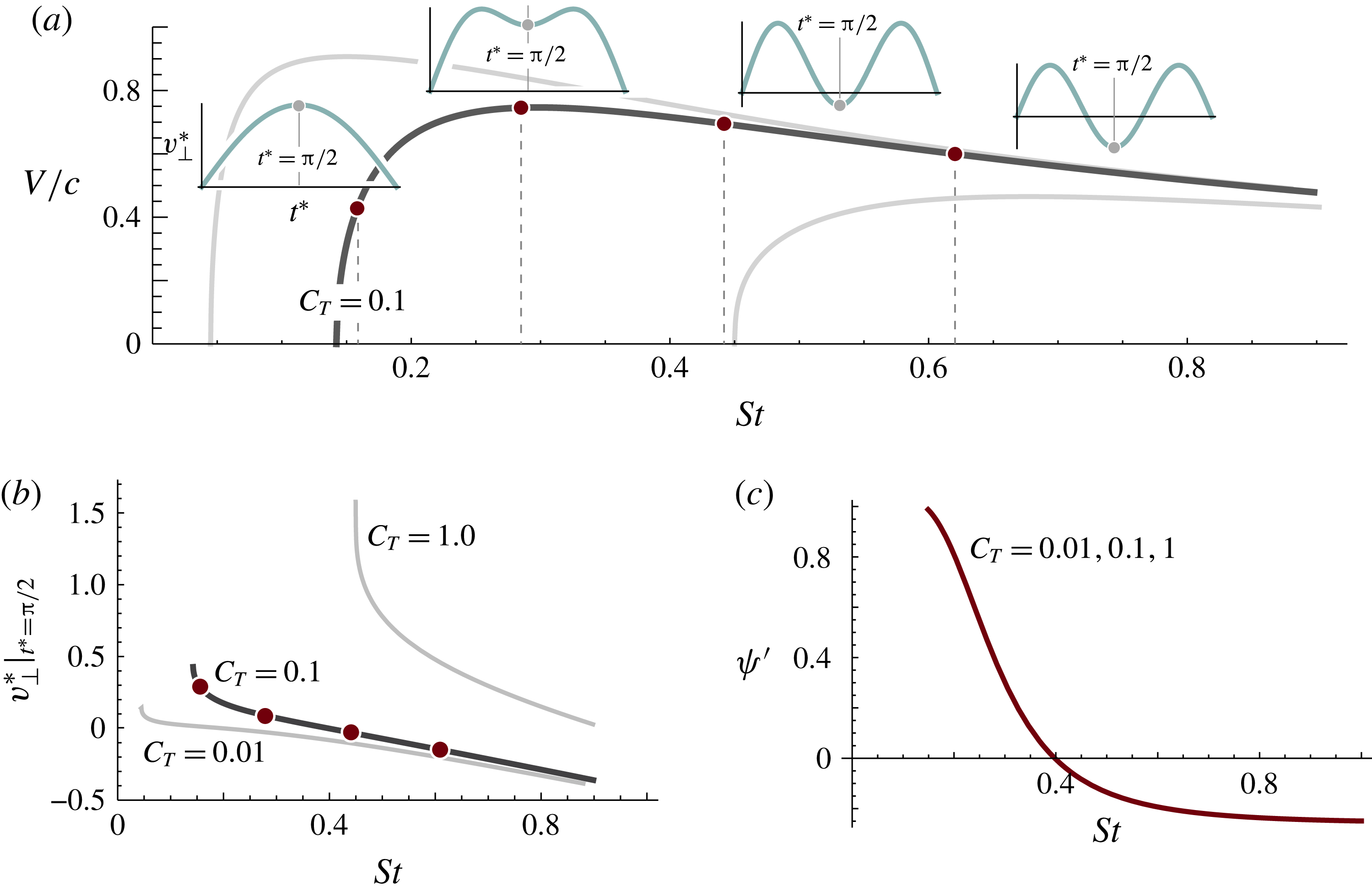
(a) The value
 $v_{\bot }^{\ast }$
at
 $t^{\ast }=\unicode[STIX]{x03C0}/2$
is unique for each point along a given constant thrust curve. (b) Curves of
 $v_{\bot }^{\ast }|_{t^{\ast }=\unicode[STIX]{x03C0}/2}$
versus
 $St$
illustrate the one-to-one mapping between
 $v_{\bot }^{\ast }|_{t^{\ast }=\unicode[STIX]{x03C0}/2}$
and profile shape along each thrust curve. (c) Normalizing
 $v_{\bot }^{\ast }|_{t^{\ast }=\unicode[STIX]{x03C0}/2}$
collapses the curves from the plot in (b) to a single line.

To construct our similarity variable,
 $\unicode[STIX]{x1D713}$
, we begin by selecting a scalar property which uniquely identifies the different
 $v_{\bot }^{\ast }$
profiles along each thrust curve. In figure 7(a) we see that the magnitude of
 $v_{\bot }^{\ast }$
at
 $t^{\ast }=\unicode[STIX]{x03C0}/2$
decreases monotonically as
 $St$
increases. We verify this in figure 7(b), where
 $v_{\bot }^{\ast }|_{t^{\ast }=\unicode[STIX]{x03C0}/2}$
is plotted along three different thrust contours. To collapse these curves to a single line, we normalize
 $v_{\bot }^{\ast }|_{t^{\ast }=\unicode[STIX]{x03C0}/2}$
against its derivative at
 $t^{\ast }=0$
:
 $$\begin{eqnarray}\unicode[STIX]{x1D713}^{\prime }=v_{\bot }^{\ast }|_{t^{\ast }=\unicode[STIX]{x03C0}/2}\left(\frac{\unicode[STIX]{x2202}v_{\bot }^{\ast }}{\unicode[STIX]{x2202}t}\bigg|_{t^{\ast }=0}\right)^{-1}.\end{eqnarray}$$
The collapsed curves are shown in figure 7(c). To complete our similarity variable, we make one last change. Profile shapes relevant to natural swimmers correspond to the range
 $-\infty <\unicode[STIX]{x1D713}^{\prime }<1$
. We apply a change of variables to alter this range to
 $0<\unicode[STIX]{x1D713}<\infty$
for the sake of convenience. This yields the final result:
 $$\begin{eqnarray}\unicode[STIX]{x1D713}=1-\frac{\sin (\unicode[STIX]{x1D6FD})-\unicode[STIX]{x03C0}St\cos (\unicode[STIX]{x1D6FD})}{\unicode[STIX]{x1D6FD}-\unicode[STIX]{x03C0}St},\quad \text{where }\unicode[STIX]{x1D6FD}=\unicode[STIX]{x03C0}\frac{V}{c}St.\end{eqnarray}$$
In figure 8, we can now see that each value of
 $\unicode[STIX]{x1D713}$
corresponds to a single common
 $v_{\bot }^{\ast }$
profile across all thrust contours.
Each value of
 $\unicode[STIX]{x1D713}$
corresponds to a single self-similar
 $v_{\bot }^{\ast }$
profile across all thrust contours. Each set of
 $V/c$
–
 $St$
points identified in (a) corresponds to a
 $v_{\bot }^{\ast }$
profile plotted in (b).

5.1 Solving for optimal
 $\unicode[STIX]{x1D713}$

If the optimal
 $V/c$
–
 $St$
relationship corresponds to a line of fixed profile shape it should reduce to a constant,
 $\unicode[STIX]{x1D713}=\unicode[STIX]{x1D713}_{opt}$
. To solve for the value of this constant we consider the form of the thrust and power coefficients. When expressed in terms of
 $\unicode[STIX]{x1D6FD}$
and
 $St$
they consist of polynomials in
 $St$
with coefficients defined by nonlinear functions of
 $\unicode[STIX]{x1D6FD}$
:
 $$\begin{eqnarray}\displaystyle & \displaystyle C_{T}(\unicode[STIX]{x1D6FD},St)=f_{2}(\unicode[STIX]{x1D6FD})St^{2}+f_{1}(\unicode[STIX]{x1D6FD})St+f_{0}(\unicode[STIX]{x1D6FD}), & \displaystyle\end{eqnarray}$$
 $$\begin{eqnarray}\displaystyle & \displaystyle C_{P}(\unicode[STIX]{x1D6FD},St)=g_{3}(\unicode[STIX]{x1D6FD})St^{3}+g_{2}(\unicode[STIX]{x1D6FD})St^{2}+g_{1}(\unicode[STIX]{x1D6FD})St+g_{0}(\unicode[STIX]{x1D6FD}). & \displaystyle\end{eqnarray}$$
At the optimum, the gradient of the objective,
 $C_{P}$
, is orthogonal to the constraint,
 $C_{T}=Li$
, giving the following optimality condition:
 $$\begin{eqnarray}\unicode[STIX]{x1D735}C_{P}\boldsymbol{\cdot }\unicode[STIX]{x1D64D}\unicode[STIX]{x1D735}C_{T}=0,\quad \text{where }\unicode[STIX]{x1D64D}=\left[\begin{array}{@{}cc@{}}0 & -1\\ 1 & 0\end{array}\right].\end{eqnarray}$$
Using this condition in combination with equations (5.2)–(5.4), we can solve for
 $\unicode[STIX]{x1D713}_{opt}$
in terms of the tail pitch
 $\unicode[STIX]{x1D6FD}$
. From the resulting solution,
 $\unicode[STIX]{x1D713}_{opt}=f(\unicode[STIX]{x1D6FD})$
, we find that the optimum is not analytically self-similar, but the variation in
 $\unicode[STIX]{x1D713}_{opt}$
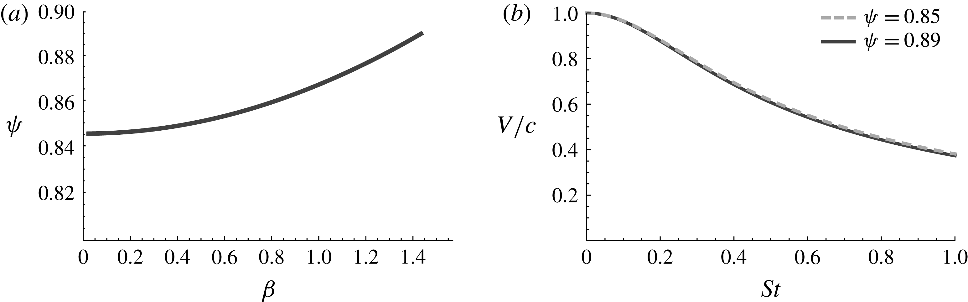
is small enough to be ignored for all practical applications. In figure 9(a), the value of
 $\unicode[STIX]{x1D713}_{opt}$
is plotted over the range of tail pitch relevant to swimming animals,
 $0<\unicode[STIX]{x1D6FD}<\unicode[STIX]{x03C0}/2$
. From the resulting curve we see that
 $\unicode[STIX]{x1D713}_{opt}$
varies from 0.85 to 0.89 with a mean value of 0.87. In figure 9(b), the bounds of
 $\unicode[STIX]{x1D713}_{opt}$
are plotted in the
 $V/c$
–
 $St$
plane, where we can see that they nearly overlap one another. In figure 3, we plot the curve defined by
 $\unicode[STIX]{x1D713}=0.87$
overtop the numerical optimum; the resulting comparison shows that the two solutions are effectively identical.
(a) Optimally efficient value of
 $\unicode[STIX]{x1D713}$
, plotted as a function of
 $\unicode[STIX]{x1D6FD}$
. (b) Comparison of the two limits bracketing the optimal solution. The resulting curves are nearly indistinguishable in the
 $V/c$
–
 $St$
plane.

5.2 Animal behaviour in terms of
$\unicode[STIX]{x1D713}$
and
$St$


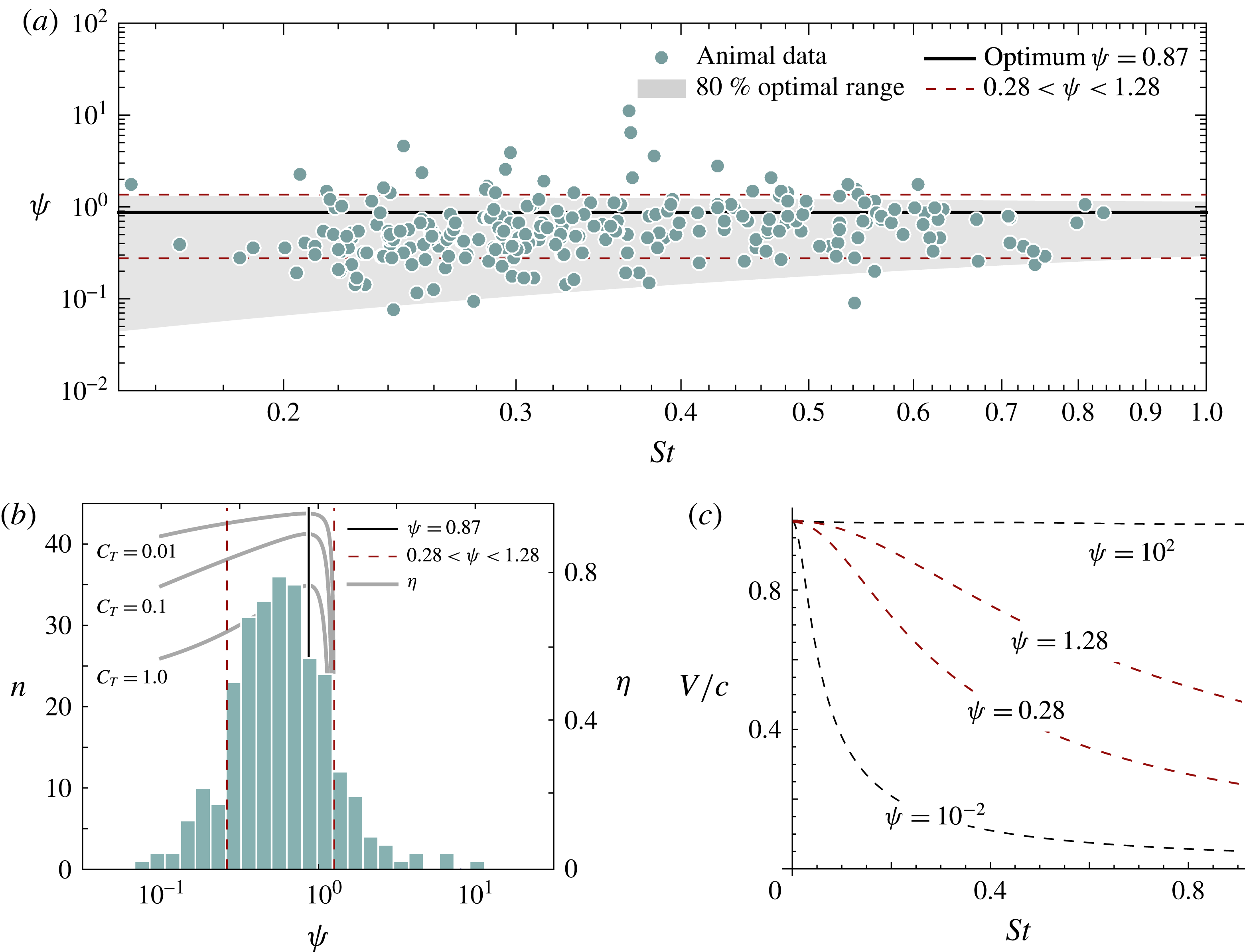
To complete our analysis we revisit the behaviour of natural swimmers in the context of our similarity variable. In figure 10, the animal dataset is presented in terms of
 $\unicode[STIX]{x1D713}$
and
 $St$
. From the resulting plot we see that animal behaviour is distributed along the optimum at
 $\unicode[STIX]{x1D713}=0.87$
, and appears to be independent of
 $St$
, as predicted. There is a relatively large degree of scatter, but this is to be expected given that we have used the slip ratio to approximate the tail pitch of the animals. As stated earlier, slip often varies along the length of the body and different methods of quantifying slip can influence the measured value by up to 10 %–20 % (Webb et al.
Reference Webb, Kostecki and Stevens1984).
(a) Animal data mapped to the
 $\unicode[STIX]{x1D713}$
–
 $St$
plane. (b) Histogram of
 $\unicode[STIX]{x1D713}$
values from animal data (
 $n_{total}=272$
). Efficiency curves are overlaid in grey. (c) Lines of constant
 $\unicode[STIX]{x1D713}$
in the
 $V/c{-}St$
plane are shown to justify the logarithmic scale used for
 $\unicode[STIX]{x1D713}$
.

In figure 10(b), we plot a histogram of
 $\unicode[STIX]{x1D713}$
for the complete dataset. The resulting distribution exhibits a clear peak in the efficient region and is well approximated by a normal distribution centred at
 $\unicode[STIX]{x1D713}=0.58$
with the range
 $\unicode[STIX]{x1D713}=0.28$
–1.28 corresponding to plus or minus one standard deviation (S.D) from the mean. The
 $\pm 1$
S.D. bounds are depicted in each of figure 10(a–c) to illustrate their form in the
 $\unicode[STIX]{x1D713}$
–
 $St$
and
 $V/c$
–
 $St$
planes. The peak at
 $\unicode[STIX]{x1D713}=0.58$
differs from the optimal value of
 $\unicode[STIX]{x1D713}=0.87$
; this can be explained by considering how efficiency varies in relation to
 $\unicode[STIX]{x1D713}$
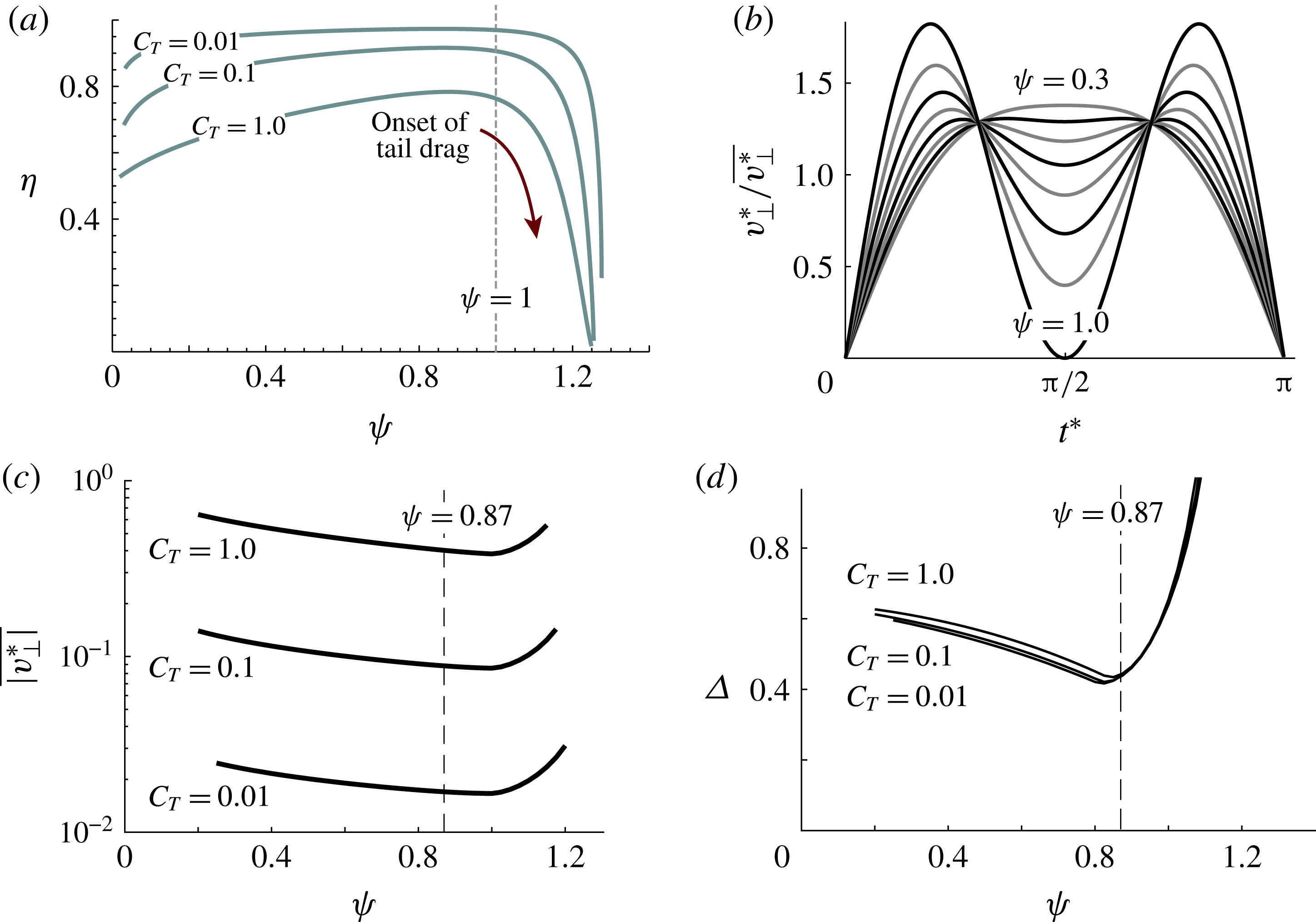
. In figure 11(a) we plot the relationship between efficiency (
 $\unicode[STIX]{x1D702}$
) and
 $\unicode[STIX]{x1D713}$
for three different levels of thrust output. The resulting curves converge to 50 % efficiency at
 $\unicode[STIX]{x1D713}=0$
and drop to 0 % efficiency at
 $\unicode[STIX]{x1D713}\approx 1.27$
, with a broad plateau between these limits. The sharp drop in efficiency past
 $\unicode[STIX]{x1D713}=1$
is caused by the onset of drag production at the tail. Using equation (5.2) it can be shown that
 $\unicode[STIX]{x1D713}=1$
corresponds to the negative thrust threshold defined in (4.5). As discussed in § 4, this threshold marks the point where
 $v_{\bot }^{\ast }|_{t^{\ast }=\unicode[STIX]{x03C0}/2}$
drops below zero and the animal begins to generate negative thrust. When swimming at the theoretically optimal value of
 $\unicode[STIX]{x1D713}=0.87$
, small changes in kinematics can push an animal into this drag production region. We hypothesize that animals insulate themselves from this effect by choosing slightly lower
 $\unicode[STIX]{x1D713}$
values. In this range efficiency is still close to optimal, but far more robust to kinematic deviations.
As highlighted earlier, optimally efficient swimmers tend to minimize both the average magnitude of
 $v_{\bot }^{\ast }$
and variations in thrust output
 $C_{T}^{i}$
. In figure 11(c,d) we plot these quantities along lines of constant thrust, over a range of
 $\unicode[STIX]{x1D713}$
values. From the resulting curves we see that both quantities exhibit a relatively flat region near the optimum at
 $\unicode[STIX]{x1D713}=0.87$
. This is consistent with the broad efficiency plateaus shown in the top left. Although there is a single mathematically optimal
 $v_{\bot }^{\ast }$
profile, in practical terms there is actually a range of self-similar profiles which provide near-optimal performance. The limits of this near-optimal range are dependent on
 $Li$
; however, as a rule of thumb the range
 $\unicode[STIX]{x1D713}=0.3$
–1 provides at least 80 % optimal efficiency across the full range of animals considered here. The
 $v_{\bot }^{\ast }$
profiles within these limits are shown in figure 11(b), where we can see that they range from a single flattened peak, to a double peak with a large central dip.
(a) Efficiency versus
 $\unicode[STIX]{x1D713}$
for three different levels of thrust output. The curves exhibit a plateau in the optimal region with a sharp drop-off at the limits,
 $\unicode[STIX]{x1D713}=0$
and
 $\unicode[STIX]{x1D713}\approx 1.27$
. (b)
 $v_{\bot }^{\ast }$
profiles within the efficient range
 $\unicode[STIX]{x1D713}=0.3$
–1.0. (c) Average magnitude of
 $v_{\bot }^{\ast }$
plotted against
 $\unicode[STIX]{x1D713}$
along constant thrust curves. (d) Average variation in
 $C_{T}$
plotted against
 $\unicode[STIX]{x1D713}$
along constant thrust curves;
 $\unicode[STIX]{x1D6E5}$
is defined in (4.4).

(a,b) Swimming motions and
 $v_{\bot }$
profile of 5 dpf zebrafish larva from open-access dataset of van Leeuwen, Voesenek & Müller (Reference van Leeuwen, Voesenek and Müller2015). Variable
 $L$
corresponds to the body length of the swimmer. (c,d) Normal velocity profiles from individual recordings of 4 and 5 dpf specimens. (e,f) Mean velocity profile across all swimming recordings for 4 and 5 dpf specimens.

The slip ratio and Strouhal number can only provide an approximate description of tail-tip motion; however, the kinematic data required to directly extract full
 $v_{\bot }$
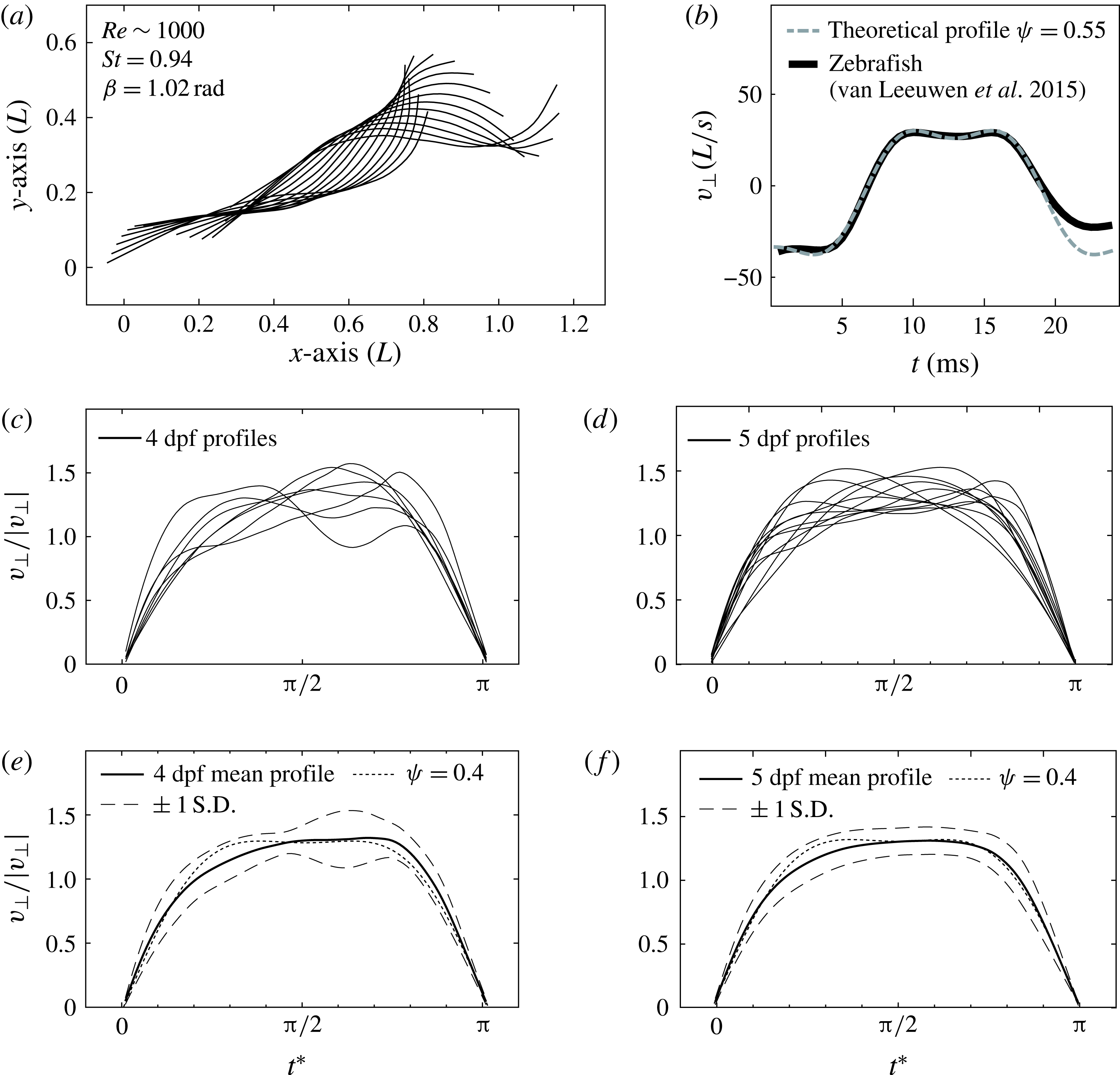
profiles are typically not included in published work. One exception to this is a study by van Leeuwen et al. (Reference van Leeuwen, Voesenek and Müller2015) on the swimming motions of larval zebrafish. Alongside their published analysis, van Leeuwen et al. (Reference van Leeuwen, Voesenek and Müller2015) include a full open-access dataset of steady-swimming video captures. The dataset contains kinematics for larval specimens at various stages of development, ranging from 1 to 5 days postfertilization (dpf). The swimming motions of a 5 dpf specimen are shown in figure 12(a), with the corresponding
 $v_{\bot }$
profile shown in figure 12(b). The central dip associated with optimality under Lighthill’s model is clearly visible; the shape of the measured profile is well approximated by the theoretical profile at
 $\unicode[STIX]{x1D713}=0.55$
. In this particular case the profile is quite clear and symmetric; however, this shape can vary significantly across different swimming recordings. To address this, we consider the average profile produced by the 4 dpf and 5 dpf specimens. These groups are chosen because they consistently swam in the highest Reynolds number range (
 $Re\approx 10^{3}$
) among all specimens. The dataset contains 8 unique recordings of 4 dpf specimens and 11 unique recordings of 5 dpf specimens. The mean profiles measured from each of these recordings are shown in figure 12(c,d). There is significant variation among the profiles; however, the majority of them exhibit the predicted flattened or depressed region at
 $t^{\ast }=\unicode[STIX]{x03C0}/2$
. The average profile for all recordings within each group is shown in figure 12(e,f). The resulting curves exhibit the central plateau associated with efficient swimming and are reasonably approximated by the theoretical profile corresponding to
 $\unicode[STIX]{x1D713}=0.4$
. This value is close to the observed peak in the distribution of figure 10 and falls within the predicted
 $80\,\%$
optimal range.
5.3 Characterizing optimal swimming behaviours
In the case of foil-tailed swimmers, previous work has shown that
 $St$
is strongly linked to optimality through its impact on the vortex wake (Triantafyllou et al.
Reference Triantafyllou, Triantafyllou and Yue2000). In contrast to this, our analysis suggests that for slender swimmers the link between optimality and
 $St$
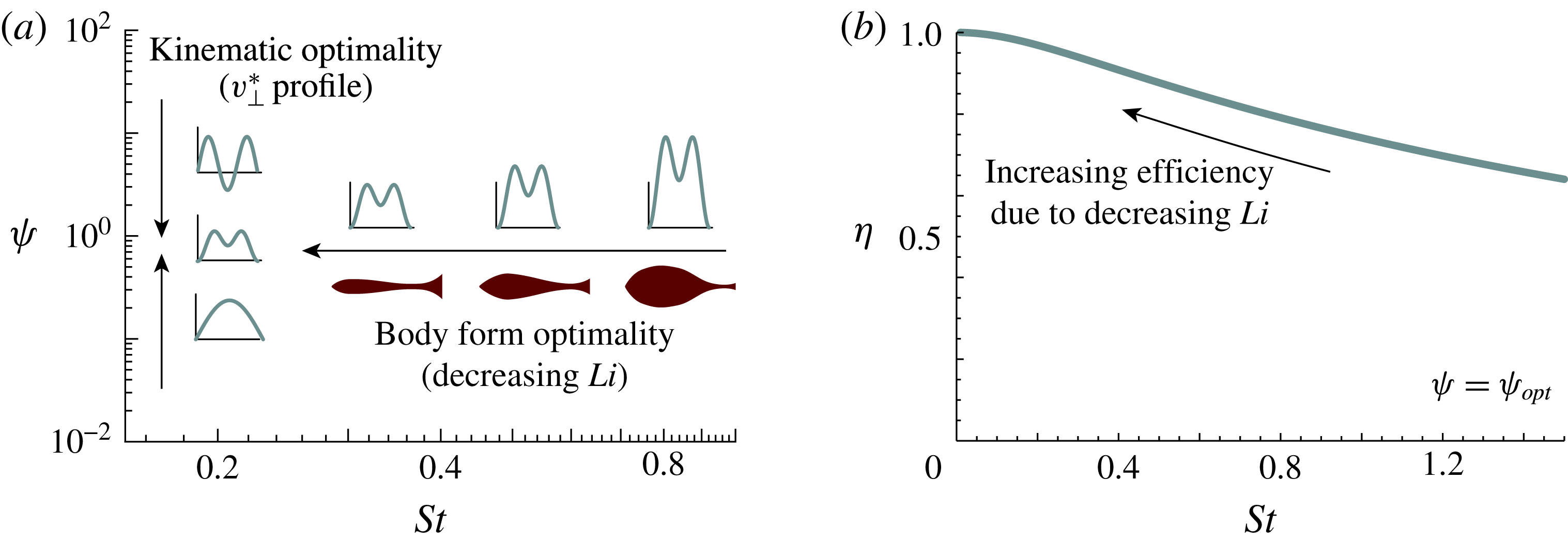
may be much weaker. Within Lighthill’s model the Strouhal number of an optimal swimmer is simply determined by thrust–drag balance. As shown in figure 13(a), the vertical axis of our kinematic space,
 $\unicode[STIX]{x1D713}$
, describes profile shape, while the horizontal axis,
 $St$
, describes profile magnitude. A swimming animal which tunes its undulations to sit in the optimal
 $\unicode[STIX]{x1D713}$
region will naturally settle at an appropriate
 $St$
value, where the thrust output of its tail balances the drag of its body.
That being said, this does not mean that
 $St$
is completely decoupled from swimming performance. As shown in figure 13(b), animals with body shapes and tail sizes which allow them to swim in the lower-
 $St$
range are significantly more efficient than their high-
 $St$
counterparts. Furthermore, figure 10 shows that the
 $\unicode[STIX]{x1D702}>0.8\unicode[STIX]{x1D702}_{max}$
bounds span a much wider range when
 $St$
is low; meaning that animals in this region remain reasonably efficient across a much broader range of kinematics. Within the context of Lighthill’s model,
 $\unicode[STIX]{x1D713}$
and
 $St$
can be thought of as characterizing the optimality of two distinct properties of a swimming animal. While
 $\unicode[STIX]{x1D713}$
describes the optimality of an animal’s swimming movements,
 $St$
describes the optimality of its body form. As shown in figure 13(a), low
 $St$
values indicate that an animal has a streamlined body and large tail, designed for high propulsive efficiency.
(a)
 $\unicode[STIX]{x1D713}$
describes the shape of a swimming animal’s
 $v_{\bot }^{\ast }$
profile, while
 $St$
determines its magnitude. (b) Peak achievable efficiency is higher for animals with a tail loading,
 $Li$
, which allows them to swim at lower
 $St$
values.

6 Conclusion
Throughout the past century researchers have sought a reductionist description of swimming motion. Beginning with Lighthill’s classical small-amplitude analysis, which identified the slip ratio as the central kinematic variable, followed by breakthroughs of Triantafyllou and his collaborators on the significance of the Strouhal number. Here we have shown that, for slender animals, optimally efficient swimming kinematics can be reduced to a new parameter,
 $\unicode[STIX]{x1D713}$
, defined by a function of both
 $V/c$
and
 $St$
. This new variable,
 $\unicode[STIX]{x1D713}$
, characterizes how tail-tip velocity varies throughout the swimming motion. Using Lighthill’s large-amplitude model, we have shown that near-optimal efficiency is achieved in the range
 $0.3<\unicode[STIX]{x1D713}<1.0$
, where the average magnitude of the tail-tip velocity is minimized and the instantaneous thrust coefficient varies as little as possible throughout the swimming stroke.
This link between thrust variation and efficiency is shared by many other biological systems. A classical example is Keller’s analysis of optimal running strategy for human athletes (Keller Reference Keller1974). Keller shows that the best overall strategy for long races is to run at a constant velocity. This result stems from a mathematical problem structure which is similar to the one outlined here. For swimming animals, this result suggests that improved gaits could be developed by including additional harmonics in the tail motion, with the goal of reducing thrust variation. For foil-tail swimmers, Prempraneerach, Hover & Triantafyllou (Reference Prempraneerach, Hover and Triantafyllou2003) demonstrate that modifying kinematics to smooth the angle of attack profile can significantly improve swimming efficiency.
In terms of next steps, significant insight could be gained from an experimental study of the concepts laid out here. There is very little experimental data on the hydrodynamics of undulating elongated bodies; however, a number of parametric studies on flapping foils have produced results that resemble the thrust and efficiency maps predicted by Lighthill’s model. Bandyopadhyay et al. (Reference Bandyopadhyay, Beal, Hrubes and Mangalam2012) study the propulsive performance of a sinusoidally flapping wing over a grid of
 $St$
and
 $\unicode[STIX]{x1D6FD}$
values ranging from
 $St=0.2$
–1.4 and
 $\unicode[STIX]{x1D6FD}=0.25{-}1.5$
. They show that both parameters are required to characterize the efficiency of the foil. The resulting contours of thrust and efficiency are qualitatively similar to those of Lighthill’s model, with the optimally efficient region lying along a
 $St-\unicode[STIX]{x1D6FD}$
curve which is analogous to the
 $St-V/c$
relationship identified here. Hover, Haugsdal & Triantafyllou (Reference Hover, Haugsdal and Triantafyllou2004) conduct a parametric study of flexible foils over a similar parameter range; again the resulting contours and optimal efficiency curve are similar to those predicted by Lighthill’s theory. This correspondence is somewhat surprising given the differences between the two systems. For foil-tailed swimmers, propulsive force is generated in the direct vicinity of vortex shedding. Based on this, wake effects should be critical to the swimming performance of these animals. Lighthill predicts the existence of a similar vortex wake for elongated swimmers, but his analysis takes its effects to be negligible. Since thrust is generated along the entire length of the body, he assumes that vortices shed from the tail propagate away without significantly altering the force distribution over the body surface. Any firm conclusions on the relationship between these systems will undoubtedly require further experimental or computational investigation; however, the striking predictions of Lighthill’s models suggest that it captures at least some of the physical effects which motivate the behaviour of efficient slender animals.
Acknowledgements
This material is based in part upon work supported by the National Science Foundation under grant no. DMS-1517842. Any opinions, findings, and conclusions or recommendations expressed in this material are those of the author(s) and do not necessarily reflect the views of the National Science Foundation.
Supplementary materials
Supplementary materials are available at https://doi.org/10.1017/jfm.2018.14.
Appendix A. Relating tail angle and slip ratio
Within our swimming model we define the motions of the tail’s trailing edge in terms of angle
 $\unicode[STIX]{x1D703}(t)$
and position
 $\boldsymbol{r}(t)$
:
 $$\begin{eqnarray}\boldsymbol{r}(t)=Vt\;\hat{\boldsymbol{e}}_{x}+A\cos (2\unicode[STIX]{x03C0}ft)\;\hat{\boldsymbol{e}}_{y}\;,\quad \text{and}\quad \unicode[STIX]{x1D703}(t)=\unicode[STIX]{x1D6FD}\sin (2\unicode[STIX]{x03C0}ft).\end{eqnarray}$$
The amplitude of the pitching motion is determined by
 $\unicode[STIX]{x1D6FD}$
; however, this kinematic quantity is rarely measured in biological studies. To compare the predictions of the model to existing data we relate the pitching amplitude
 $\unicode[STIX]{x1D6FD}$
to the slip ratio
 $V/c$
which is more commonly recorded. This relation is derived by assuming that the body undulations of swimming animals can be approximated as a sinusoidal wave. Here, we consider two possible mathematical definitions for this wave:
 $$\begin{eqnarray}\displaystyle & \displaystyle y_{1}(x,t)=A(x)\cos \left(2\unicode[STIX]{x03C0}\left(ft-\frac{x}{\unicode[STIX]{x1D706}}\right)\right), & \displaystyle\end{eqnarray}$$
 $$\begin{eqnarray}\displaystyle & \displaystyle y_{2}(s,t)=A(s)\cos \left(2\unicode[STIX]{x03C0}\left(ft-\frac{s}{\unicode[STIX]{x1D706}}\right)\right). & \displaystyle\end{eqnarray}$$
In the first definition, body position is taken to be a sinusoidal function of the inertial coordinate
 $x$
, while in the second it is taken to be a sinusoidal function of the body coordinate
 $s$
. Both approaches provide reasonable approximations of swimming motion; however, they yield slightly different relationships between
 $\unicode[STIX]{x1D6FD}$
and
 $V/c$
. To define these relationships, we first define the body angle in terms of the body wavefunctions:
 $$\begin{eqnarray}\unicode[STIX]{x1D703}_{1}(x,t)=\tan ^{-1}\left(\frac{\unicode[STIX]{x2202}y_{b}}{\unicode[STIX]{x2202}x}\right)\quad \text{and}\quad \unicode[STIX]{x1D703}_{2}(s,t)=\sin ^{-1}\left(\frac{\unicode[STIX]{x2202}y_{b}}{\unicode[STIX]{x2202}s}\right),\end{eqnarray}$$
 $$\begin{eqnarray}\displaystyle & \displaystyle \unicode[STIX]{x1D703}_{1}(x,t)=\tan ^{-1}\left(\frac{2\unicode[STIX]{x03C0}A(x)}{\unicode[STIX]{x1D706}}\sin \left(2\unicode[STIX]{x03C0}\left(ft-\frac{x}{\unicode[STIX]{x1D706}}\right)\right)+\frac{\text{d}A(x)}{\text{d}x}\sin \left(2\unicode[STIX]{x03C0}\left(ft-\frac{x}{\unicode[STIX]{x1D706}}\right)\right)\right), & \displaystyle\end{eqnarray}$$
 $$\begin{eqnarray}\displaystyle & \displaystyle \unicode[STIX]{x1D703}_{2}(s,t)=\sin ^{-1}\left(\frac{2\unicode[STIX]{x03C0}A(s)}{\unicode[STIX]{x1D706}}\sin \left(2\unicode[STIX]{x03C0}\left(ft-\frac{s}{\unicode[STIX]{x1D706}}\right)\right)+\frac{\text{d}A(s)}{\text{d}s}\sin \left(2\unicode[STIX]{x03C0}\left(ft-\frac{x}{\unicode[STIX]{x1D706}}\right)\right)\right). & \displaystyle\end{eqnarray}$$
The amplitude derivative at the trailing edge
 $(s=\ell ,\;x=\ell )$
is assumed to be zero such that the wave is consistent with the motion defined in (A 1).
 $\unicode[STIX]{x1D6FD}$
is taken to be equal to the peak value of the body angle at the tail. This yields the following relations for
 $\unicode[STIX]{x1D6FD}$
and
 $V/c$
:
 $$\begin{eqnarray}\displaystyle & \displaystyle \unicode[STIX]{x1D6FD}_{1}=\arctan \left(\frac{2\unicode[STIX]{x03C0}A(\ell )}{\unicode[STIX]{x1D706}}\right)=\arctan \left(\unicode[STIX]{x03C0}\frac{V}{c}St\right), & \displaystyle\end{eqnarray}$$
 $$\begin{eqnarray}\displaystyle & \displaystyle \unicode[STIX]{x1D6FD}_{2}=\arcsin \left(\frac{2\unicode[STIX]{x03C0}A(\ell )}{\unicode[STIX]{x1D706}}\right)=\arcsin \left(\unicode[STIX]{x03C0}\frac{V}{c}St\right). & \displaystyle\end{eqnarray}$$
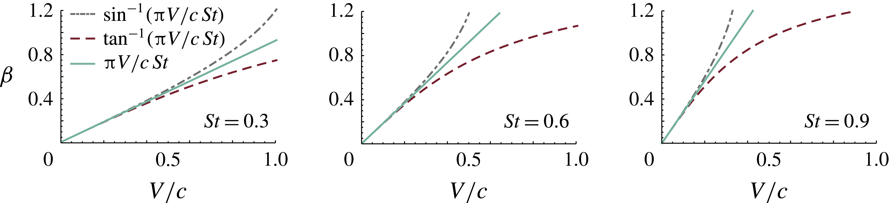
In figure 14 the two relations are compared to one another at three different values of
 $St$
. For
 $\unicode[STIX]{x03C0}V/cSt<1$
the two relations are similar; however, as this term grows the two relations begin to diverge. In each plot we include a third curve representing the simplified relation,
 $\unicode[STIX]{x1D6FD}=\unicode[STIX]{x03C0}V/cSt$
. Over the range of
 $\unicode[STIX]{x1D6FD}$
values relevant to swimming, this simplified relation provides a compromise between the two previously presented alternatives while also being much simpler mathematically. Based on this, we apply the simplified relation for
 $\unicode[STIX]{x1D6FD}$
and
 $V/c$
throughout our analysis.
Comparison of alternative relations for slip ratio and pitch angle amplitude.

Appendix B. How do efficient swimmers generate thrust?
Within Lighthill’s model swimming animals produce thrust through two distinct sources: the normal force (
 $\boldsymbol{F}_{n}$
) and a tangential force (
 $\boldsymbol{F}_{t}$
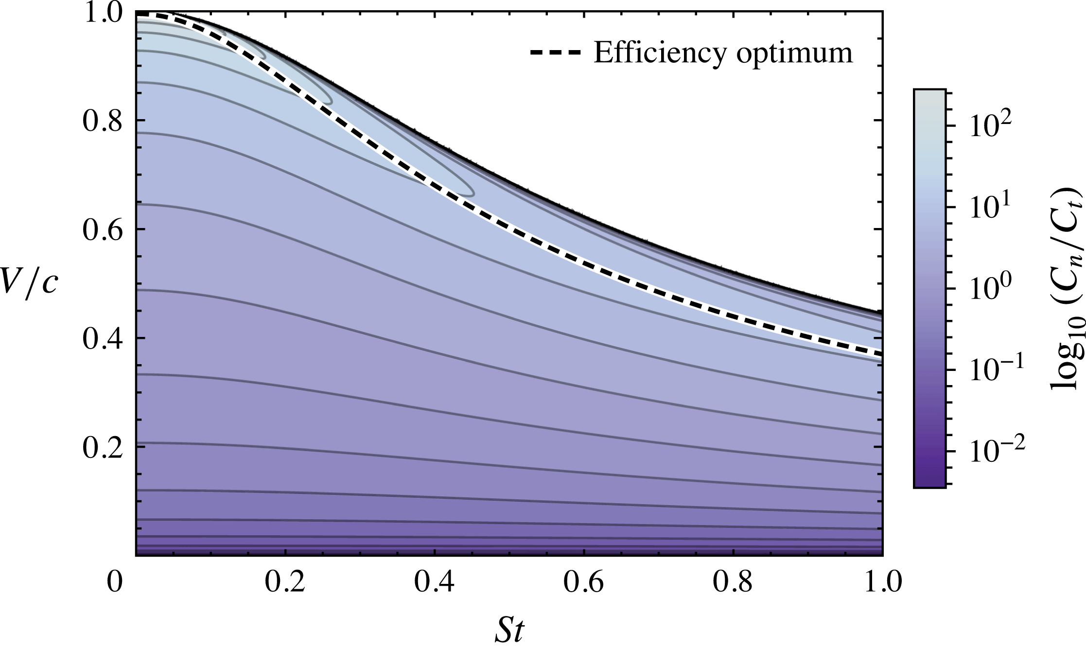
). These two terms compose the thrust coefficient within our optimization problem. In figure 15 we plot the ratio of the thrust components over the
 $St-V/c$
plane. This ratio
 $C_{n}/C_{t}$
is defined as
 $$\begin{eqnarray}\frac{C_{n}}{C_{t}}=\frac{\displaystyle \int _{0}^{2\unicode[STIX]{x03C0}}v_{\Vert }^{\ast }v_{\bot }^{\ast }\sin (\unicode[STIX]{x1D703}(t^{\ast }))\,\text{d}t^{\ast }}{\displaystyle \int _{0}^{2\unicode[STIX]{x03C0}}\frac{1}{2}v_{\bot }^{\ast 2}\cos (\unicode[STIX]{x1D703}(t^{\ast }))\,\text{d}t^{\ast }}.\end{eqnarray}$$
The contours of figure 15 illustrate how the relative contributions of the two thrust sources vary in relation to kinematics. Within the most efficient region of the map, the normal force accounts for almost all of the thrust generated by the animal. The advantage of thrust from this source can be shown by considering the thrust-to-power ratio
 $C_{T}/C_{P}$
:
 $$\begin{eqnarray}\frac{C_{T}}{C_{P}}=\frac{C_{t}}{C_{P}}+\frac{C_{n}}{C_{P}}.\end{eqnarray}$$
The two terms within
 $C_{T}/C_{P}$
represent the thrust-to-power ratio of each thrust source. Under the constraints
 $St\geqslant 0$
and
 $0\leqslant \unicode[STIX]{x1D6FD}\leqslant \unicode[STIX]{x03C0}/2$
, the upper bound of
 $C_{t}/C_{P}$
is one, while the upper bound of
 $C_{n}/C_{P}$
is infinity. Substituting these bounds into (2.15) reveals that thrust from the tangential force can never exceed
 $50\,\%$
efficiency, while thrust from the normal force can approach 100 %.
Ratio of thrust from the tangential and normal forces. In the optimally efficient region, the normal force is roughly 10–100 times greater than tangential force.

Appendix C. Lighthill’s large-amplitude elongated-body theory
The notation used throughout our analysis is differs from that of Lighthill (Reference Lighthill1971). We define the average thrust produced by the swimmer as follows, where
 $m$
is the hydrodynamic mass at the trailing edge:
 $$\begin{eqnarray}\displaystyle & \displaystyle \overline{T}=f\int _{0}^{1/f}\left(\boldsymbol{F}_{n}(t)+\boldsymbol{F}_{t}(t)\right)\boldsymbol{\cdot }\hat{\boldsymbol{e}}_{x}\,\text{d}t, & \displaystyle\end{eqnarray}$$
 $$\begin{eqnarray}\displaystyle & \displaystyle \boldsymbol{F}_{n}(t)=m\;\left(v_{\Vert }^{\ast }v_{\bot }^{\ast }\right)\hat{\boldsymbol{e}}_{\bot }, & \displaystyle\end{eqnarray}$$
 $$\begin{eqnarray}\displaystyle & \displaystyle \boldsymbol{F}_{t}(t)=m\;\left({\textstyle \frac{1}{2}}\;v_{\bot }^{\ast \;2}\right)\hat{\boldsymbol{e}}_{\Vert }, & \displaystyle\end{eqnarray}$$
and
 $$\begin{eqnarray}\hat{\boldsymbol{e}}_{\bot }=[\sin \unicode[STIX]{x1D703}\;\;\cos \unicode[STIX]{x1D703}],\quad \hat{\boldsymbol{e}}_{\Vert }=[-\cos \unicode[STIX]{x1D703}\;\;\sin \unicode[STIX]{x1D703}].\end{eqnarray}$$
Using equation (C 4), the thrust integral reduces to the following scalar result:
 $$\begin{eqnarray}\overline{T}=m\int _{0}^{2\unicode[STIX]{x03C0}}\left(v_{\Vert }v_{\bot }\sin (\unicode[STIX]{x1D703})+\frac{1}{2}v_{\bot }^{2}\cos (\unicode[STIX]{x1D703})\right)\text{d}t.\end{eqnarray}$$
Within Lighthill’s derivation
 $v_{\Vert }$
and
 $v_{\bot }$
are denoted by the variables
 $u$
and
 $w$
and the projections
 $\cos \unicode[STIX]{x1D703}$
and
 $\sin \unicode[STIX]{x1D703}$
are given by the spatial derivatives
 $\unicode[STIX]{x2202}x/\unicode[STIX]{x2202}a$
and
 $\unicode[STIX]{x2202}z/\unicode[STIX]{x2202}a$
, where
 $x$
is equivalent to our
 $x$
coordinate,
 $z$
is equivalent to our
 $y$
coordinate, and
 $a$
is a curvilinear coordinate along the swimmer’s spine. Making these substitutions we see that equation (C 5) is equivalent to the time average of the horizontal thrust component of equation (5) in Lighthill (Reference Lighthill1971):
 $$\begin{eqnarray}\overline{T}=m\int _{0}^{2\unicode[STIX]{x03C0}}\left(uw\frac{\unicode[STIX]{x2202}z}{\unicode[STIX]{x2202}a}+\frac{1}{2}w^{2}\frac{\unicode[STIX]{x2202}x}{\unicode[STIX]{x2202}a}\right)\text{d}t.\end{eqnarray}$$
Equation (7) of Lighthill (Reference Lighthill1971) reduces this to the more compact form
 $$\begin{eqnarray}\overline{T}=m\int _{0}^{2\unicode[STIX]{x03C0}}w\left(\frac{\text{d}z}{\text{d}t}-\frac{1}{2}w\frac{\unicode[STIX]{x2202}x}{\unicode[STIX]{x2202}a}\right)\text{d}t.\end{eqnarray}$$
The details of the reduction process are not included in Lighthill (Reference Lighthill1971); we provide them here to demonstrate the equivalence of the two forms. Starting with (C 5), we begin by separating
 $(1/2)v_{\bot }^{2}\cos \unicode[STIX]{x1D703}$
into two terms and factoring out
 $v_{\bot }$
:
 $$\begin{eqnarray}\overline{T}=m\int _{0}^{2\unicode[STIX]{x03C0}}v_{\bot }\left(v_{\Vert }\sin (\unicode[STIX]{x1D703})+v_{\bot }\cos (\unicode[STIX]{x1D703})-\frac{1}{2}v_{\bot }\cos (\unicode[STIX]{x1D703})\right)\text{d}t.\end{eqnarray}$$
The velocity terms in (C 8) can be expanded as follows:
 $$\begin{eqnarray}v_{\bot }=\frac{\text{d}\boldsymbol{r}}{\text{d}t}\boldsymbol{\cdot }\hat{\boldsymbol{e}}_{\bot },\quad v_{\Vert }=\frac{\text{d}\boldsymbol{r}}{\text{d}t}\boldsymbol{\cdot }\hat{\boldsymbol{e}}_{\Vert },\end{eqnarray}$$
 $$\begin{eqnarray}v_{\bot }=\frac{\text{d}x}{\text{d}t}\sin \unicode[STIX]{x1D703}+\frac{\text{d}y}{\text{d}t}\cos \unicode[STIX]{x1D703},\quad v_{\Vert }=-\frac{\text{d}x}{\text{d}t}\cos \unicode[STIX]{x1D703}+\frac{\text{d}y}{\text{d}t}\sin \unicode[STIX]{x1D703}.\end{eqnarray}$$
Substituting these expressions into (C 8) produces the following result:
 $$\begin{eqnarray}\overline{T}=m\!\int _{0}^{2\unicode[STIX]{x03C0}}\!\!v_{\bot }\!\left(\!-\frac{\text{d}x}{\text{d}t}\cos \unicode[STIX]{x1D703}\sin \unicode[STIX]{x1D703}+\frac{\text{d}y}{\text{d}t}\sin ^{2}\unicode[STIX]{x1D703}+\frac{\text{d}x}{\text{d}t}\sin \unicode[STIX]{x1D703}\cos \unicode[STIX]{x1D703}+\frac{\text{d}y}{\text{d}t}\cos ^{2}\unicode[STIX]{x1D703}-\frac{1}{2}v_{\bot }\cos (\unicode[STIX]{x1D703})\!\right)\!\text{d}t,\end{eqnarray}$$
which then collapses to
 $$\begin{eqnarray}\overline{T}=m\int _{0}^{2\unicode[STIX]{x03C0}}v_{\bot }\left(\frac{\text{d}y}{\text{d}t}-\frac{1}{2}v_{\bot }\cos (\unicode[STIX]{x1D703})\right)\text{d}t.\end{eqnarray}$$
Converting this result to Lighthill’s notation we see that it is equivalent to equation (7) of Lighthill (Reference Lighthill1971):
 $$\begin{eqnarray}\overline{T}=m\int _{0}^{2\unicode[STIX]{x03C0}}w\left(\frac{\text{d}z}{\text{d}t}-\frac{1}{2}w\frac{\unicode[STIX]{x2202}x}{\unicode[STIX]{x2202}a}\right)\text{d}t.\end{eqnarray}$$