Nomenclature
- A-CDM
-
Airport Collaborative Decision Making
- A-SMGCS
-
Advanced Surface Movement Guidance and Control System
- A320
-
Airbus A320 (Medium category in this study)
- A333
-
Airbus A330-300 (Heavy category in this study)
- AC
-
Aircraft (problem instance size, e.g. 40–50 AC)
- ACO
-
Ant Colony Optimisation
- ADS-B
-
Automatic Dependent Surveillance–Broadcast
- AI
-
Artificial Intelligence
- AIP
-
Aeronautical Information Publication
- ATC
-
Air Traffic Control
- ATCo
-
Air Traffic Controller
- ATM
-
Air Traffic Management
- BFOA
-
Bacterial Foraging Optimisation Algorithm
- C550
-
Cessna 550 Citation II (Light category in this study)
- CPS
-
Constrained Position Shifting
- CPU
-
Central Processing Unit
- DMAN
-
Departure Manager
- DSP
-
Departure Sequencing Problem
- DSS
-
Decision Support System
- EASA
-
European Union Aviation Safety Agency
- EI
-
Emission Index (mass of pollutant per mass of fuel, typically g/kg fuel)
- ETA
-
Estimated Time of Arrival
- ETD
-
Estimated Time of Departure
- FAA
-
Federal Aviation Administration
- FCFS
-
First-Come-First-Served
- GDSAA
-
General Directorate of State Airports Authority (Türkiye)
- H/M/L
-
Heavy / Medium / Light aircraft categories
- HC
-
Hydrocarbons (pollutant)
- HMI
-
Human–Machine Interface
- IATA
-
International Air Transport Association
- ICAO
-
International Civil Aviation Organization
- kg
-
kilogram
- kt
-
knot (nautical miles per hour)
- LNS
-
Large Neighbourhood Search
- LP
-
Linear Programming
- LTAI
-
Antalya Airport (ICAO location indicator)
- MACO
-
Multi-Ant Colony Optimisation
- MILP
-
Mixed-Integer Linear Programming
- MPS
-
Maximum Position Shift
- NOx
-
Nitrogen oxides (pollutant)
- NP-hard
-
Non-deterministic Polynomial-time hard
- R&D
-
Research and Development
- RAM
-
Random Access Memory
- SA
-
Simulated Annealing
- STD
-
Scheduled Time of Departure
- TS
-
Tabu Search
- TSAT
-
Target Start-up Approval Time
- TTOT
-
Target Take-Off Time
1.0 Introduction
The exponential expansion of international trade, coupled with the aggressive growth of both legacy and low-cost carriers, has led to a surge in global air traffic that strains the capacity of modern aviation infrastructure [1]. Within this congested environment, efficient air traffic management (ATM) is a necessity for operational safety and sustainability [Reference Yousefzadeh Aghdam, Kamel Tabbakh, Mahdavi Chabok and Kheyrabadi2]. Among the various subsystems of ATM, the management of runway capacity, specifically aircraft scheduling, has emerged as a critical bottleneck.
In daily operations, arrival flights typically take precedence over departures. This inherent prioritisation often forces departing aircraft to wait on the ground, leading to queue spillbacks and substantial delays [Reference Hong3]. Consequently, the departure sequencing problem (DSP) becomes the focal point of airport efficiency. However, optimising the DSP is complex as it requires the simultaneous coordination of aircraft types, sizes, taxi speeds and critical ground phases from pushback to takeoff [Reference Balakrishnan and Chandran4]. The process involves a rigid layer of constraints including wake turbulence separation [5], air traffic control (ATC) time windows, constrained position shifting (CPS) for airline equity and specific precedence rules [Reference Balakrishnan and Chandran6–Reference Simaiakis and Balakrishnan8].
Historically, research into solving the DSP has been polarised. On one side, exact algorithms like MILP are favoured for their ability to model detailed constraints and provide theoretically optimal solutions [Reference Cecen and Çetek9–Reference Solveling, Solak, Clarke and Johnson11]. However, exact methods are computationally expensive for large-scale NP-hard instances [Reference Ikli, Mancel, Mongeau, Olive and Rachelson12, Reference Sun, Wei and Jing13] and generally function as ‘black boxes’ that do not reveal the operational logic behind the schedule, creating a trust barrier for human controllers [Reference Goerigk and Hartisch14–Reference Lumbreras and Ciller16]. On the other side, heuristics and metaheuristics offer speed and understandable steps but traditionally rely on simplified feasibility checks. These simplifications often fail to capture system-wide dynamics such as optimal ground-holding strategies, potentially leading to sub-optimal plans [Reference Gotteland, Durand, Page and Alliot17–Reference García, Berlanga, Molina and Casar19].
To resolve this dichotomy, this study introduces a hybrid MILP-in-the-loop matheuristic framework inspired by recent advances in explainable metaheuristics [Reference Almeida, Soares, Lezama, Limmer, Rodemann and Vale20, Reference Fyvie, McCall, Christie, Brownlee and Singh21] as illustrated in Fig. 1. We develop four specific constraint-aware and adaptive variants of tabu search (TS), simulated annealing (SA), multi-ant colony optimisation (MACO) and bacterial foraging optimisation (BFOA). Unlike standard implementations, these algorithms are engineered with adaptive mechanisms to efficiently explore the search space using interpretable moves while a restricted MILP evaluator guarantees rigorous validation. This aligns with findings that controllers prefer tools that match their mental models [Reference Westin, Borst and Hilburn22], bridging the gap between numerical precision and operational explainability.
Schematic of the matheuristic loop. The metaheuristic proposes a CPS-compliant departure order; the restricted MILP returns optimal timings and holds for that fixed order; the resulting hold-fuel objective is fed back to guide the next move.

Figure 1 Long description
The flowchart depicts the process of optimizing aircraft scheduling in air traffic management using a matheuristic loop. The process begins with a matheuristic search that explores CPS-compliant departure orders via swap/insert moves. This proposed departure order is then evaluated by a restricted MILP evaluator, which optimizes timings and holds under full wake, taxi, and CPS constraints. The resulting hold-fuel cost and feasible schedule are fed back to guide the next move in the matheuristic search. This iterative process continues until the time or evaluation budget is reached. The final output is a controller-facing schedule that includes hold times and locations, CPS-compliant position shifts, runway/taxi conflict status, and deviations from estimated takeoff times.
2.0 Literature review
Matheuristics, a blend of mathematical programming and heuristic methods, have gained prominence in solving complex combinatorial optimisation problems across various domains [Reference Boschetti and Maniezzo23]. This section provides a comprehensive overview of matheuristics in general routing and scheduling applications before focusing on specific implementations in the aviation domain and identifying the gaps addressed by this study.
2.1 Matheuristics in routing, scheduling and logistics
The integration of exact solvers within heuristic frameworks has proven particularly effective in logistics. Archetti and Speranza [Reference Archetti and Speranza24] classify these approaches into decomposition, improvement and column generation-based methods. Solyal and Süral [Reference Solyal and Süral25] addressed the inventory routing problem using a matheuristic that sequentially solves different MILPs, demonstrating that this hybrid approach could outperform existing algorithms and provide new best solutions. Similarly, Boschetti and Maniezzo [Reference Boschetti and Maniezzo26] applied a matheuristic to city logistics by combining a dual ascent procedure with a randomised constructive heuristic, which proved effective in real-world scenarios. Vadseth et al. [Reference Vadseth, Andersson and Stålhane27] presented an iterative matheuristic for inventory routing that emphasised the maximum level replenishment policy and outperformed state-of-the-art exact methods on large benchmark instances. Furthermore, Moura et al. [Reference Moura, Pinto, Alves and de Carvalho28] introduced a hybrid approach for the combined bin packing and vehicle routing problem, demonstrating significant improvements in operational efficiency under real-world constraints.
In the broader context of transportation networks, Chouman and Crainic [Reference Chouman and Crainic29] developed a cutting-plane matheuristic that efficiently computes tight lower bounds, surpassing current best methods in the literature. Villegas et al. [Reference Villegas, Prins, Prodhon, Saldanha-da Gama and Santos-Pereira30] proposed a hybrid method for truck and trailer routing using a set-partitioning formulation that outperformed leading methods and highlighted the robustness of matheuristics. Additionally, Angelelli et al. [Reference Angelelli, Archetti and Peirano31] focused on freight forwarder services and validated their method on real data instances, showing its capability to offer high-quality solutions for large-scale problems within reasonable computing times.
In industrial scheduling, matheuristics often bridge the gap between theory and practice. Dang et al. [Reference Dang, van Diessen, Martagan and Adan32] tackled parallel machine scheduling using a genetic algorithm combined with linear programming, showing significant improvements over current practices. Fanjul-Peyro et al. [Reference Fanjul-Peyro, Perea and Ruiz33] proposed strategies for unrelated parallel machine scheduling that significantly outperformed mathematical models on medium-sized instances. Della Croce and Salassa [Reference Della Croce and Salassa34] introduced a variable neighbourhood search-based matheuristic for nurse rostering and demonstrated that hybrid methods can handle complex resource constraints better than pure solvers. Finally, Karlsson et al. [Reference Karlsson, Rönnberg, Stenberg and Uppman35] presented a matheuristic for large-scale avionic scheduling in integrated modular systems, effectively solving large instances and providing valuable managerial insights.
2.2 Matheuristics in aviation operations
Within the aviation sector, matheuristics have been successfully adapted to various ground and airside operations. Silva et al. [Reference da Silva, Ueno, dos Santos and de Carvalho36] addressed the aircraft landing problem (ALP) using a relax-and-fix approach that proved efficient for instances with a large number of aircraft and offered significant improvements over existing mathematical formulations. In maintenance operations, Zhang et al. [Reference Zhang, Chan, Chung and Fu37] combined ant colony optimisation with set partitioning to handle flexible cruise times. Their approach significantly improved aircraft utilisation and demonstrated high accuracy when validated with Bureau of Transportation Statistics data. Karsu and Solyal [Reference Karsu and Solyal38] employed a matheuristic for gate assignment to minimise passenger walking distances, outperforming existing algorithms in computational tests. Delgado and Mora [Reference Delgado and Mora39] applied column generation-based heuristics to air-cargo recovery and significantly improved profit margins by allowing flexible cargo assignment policies. Kyriakidou [Reference Kyriakidou40] addressed aircraft landing scheduling using variable neighbourhood search combined with interior-point methods, showing substantial improvements over traditional methods through statistical analysis.
2.3 The Gap in DSP: From black-box to explainable optimisation
Despite these successes, there is currently no matheuristic that embeds an exact MILP evaluator directly within the DSP as existing work relies predominantly on pure metaheuristics. Studies by Atkin et al. [Reference Atkin, Burke, Greenwood and Reeson41], Capr
 $\grave{i}$
and Ignaccolo [Reference Capr and Ignaccolo42] and Benlic et al. [Reference Benlic, Brownlee and Burke43] typically enforce feasibility through forward timing rules or ad-hoc repairs rather than through an exact optimisation layer. More recently, constraint-guided search frameworks have been introduced to inject structural information [Reference Riahi, Newton, Polash, Su and Sattar44], yet these still largely lack the rigorous guarantees of a MILP for complex ground-holding couplings.
Conversely, adoption barriers persist for exact methods due to their opacity. Even when a stand-alone MILP offers a detailed solution, the intermediate reordering logic remains hidden inside the branch-and-bound tree, forcing controllers to accept a ‘black box’ output without insight into the operational decisions that led to it. Recent work highlights that such opacity limits trust [Reference Aigner, Goerigk, Hartisch, Liers and Miehlich15, Reference Hurter, Degas, Guibert, Durand, Ferreira, Cavagnetto, Islam, Barua, Ahmed, Begum, Bonelli, Cartocci, Di Flumeri, Borghini, Babiloni and Aricó45] and that controllers prioritise tools aligning with their mental models [Reference Westin, Borst and Hilburn22]. To bridge this divide, this study draws on principles of explainable metaheuristics [Reference Almeida, Soares, Lezama, Limmer, Rodemann and Vale20, Reference Fyvie, McCall, Christie, Brownlee and Singh21], aiming to combine the transparency of trajectory-based search with the precision of mathematical programming.
3.0 Contribution of the study
To address the identified gap, this paper introduces a structured MILP-in-the-loop framework. Unlike previous studies that rely on simplified feasibility checks, we embed a restricted MILP as a high-fidelity evaluator within four enhanced metaheuristics. This architecture allows us to rigorously value candidate solutions while maintaining a transparent search process.
The main contributions of the study are:
-
• MILP-in-the-loop matheuristic framework: We propose a hybrid architecture where adaptive metaheuristics generate candidate sequences and a restricted MILP performs the evaluation. This novel design guarantees that every proposed solution strictly adheres to wake-turbulence, separation and ground-holding constraints, overcoming the feasibility limitations of standard heuristics (see Fig. 1).
-
• Constraint-aware and explainable search: By restricting the MILP to evaluation rather than full search, we expose the decision process. The framework operates via interpretable neighbourhood operators (e.g. CPS-compliant swaps, priority inserts), creating a traceable optimisation log where specific moves are directly linked to hold-fuel savings, addressing the transparency requirements of ATM systems.
-
• Systematic benchmarking of adaptive algorithms: We develop and rigorously compare four metaheuristic variants (enhanced TS, SA, MACO, BFOA) under a unified MILP evaluator. This controlled environment isolates the search efficiency of each algorithm, providing clear insights into their convergence behaviours under identical operational constraints.
-
• Scalability and real-world validation: Validated on calibrated data from Antalya Airport, the framework demonstrates superior scalability compared to stand-alone exact methods. In high-density scenarios where full MILP solvers struggle to close the optimality gap, the proposed algorithms converge to near-optimal solutions within tactical time limits, proving viability for real-time decision support.
-
• Decision-support ready outputs: Beyond sequencing, the model generates granular outputs including exact hold times, queue times, delays and disaggregated fuel and emission estimates (HC, CO, NOx). These metrics are designed to be directly consumable by departure manager (DMAN) tools for environmentally conscious planning.
4.0 Methodology
This section details the proposed matheuristic framework designed to solve the DSP. The central architectural principle is the decoupling of the combinatorial decision (runway sequencing) from the continuous decision (timing and holding). Four enhanced metaheuristics – enhanced TS, SA, MACO and BFOA – are responsible for exploring the discrete space of CPS-compliant departure orders, while a restricted MILP model acts as a sub-routine to optimise timings for each proposed order.
4.1 Evaluation of fixed sequences
The core innovation of our search strategy is the replacement of heuristic objective functions with an exact MILP evaluator. For any candidate permutation generated by the metaheuristic, we solve a simplified version of the DSP model where the binary ordering variables are fixed. This transforms the NP-hard sequencing problem into a computationally tractable linear programming (LP) or reduced MILP problem focusing solely on resource allocation (Fig. 1).
The evaluation protocol proceeds as follows:
-
1) The metaheuristic generates a candidate neighbour order using a constraint-aware move (e.g. a CPS-compliant swap).
-
2) This candidate order is passed to the restricted MILP, where the binary variables defining the sequence are fixed.
-
3) The restricted MILP optimises the remaining continuous variables: reaching times to each point
 $\{{t_i^p}\}$
and hold durations
$\{ {s_i^p}\}$
, ensuring optimal distribution of ground holds across the taxiway network.
-
4) The MILP returns the optimal objective value (total hold fuel) and feasibility status, which are fed back to the metaheuristic to guide the search.
-
5) Steps 1–4 repeat until the time or iteration budget is exhausted.


Frequency of evaluation: In each iteration, the metaheuristic filters candidates using quick feasibility checks (e.g. CPS bounds). Only promising candidates trigger a restricted-MILP solve. To ensure computational efficiency compatible with real-time operations, the MILP solver is warm-started from the previous solution, and the total number of MILP calls is capped by a global budget.
Computing environment: All experiments were performed on a Windows workstation equipped with an 11th Gen Intel® Core
 $^{TM}$
i7-1185G7 CPU (3.00 GHz) and 64 GB of RAM. The algorithms were implemented in Python 3.11 using Pyomo and solved with Gurobi Optimizer (v12.0.3). Default solver parameters were used, except for the TimeLimit, which was kept consistent across all runs to ensure comparability.
4.2 MILP model
We formulate the DSP on a time–space representation of the airport surface. The model minimises total ground-hold fuel while enforcing runway wake separations, multi-point ground conflict separations and CPS. Below we define all sets, indices, parameters and decision variables before presenting the constraints.
Sets and indices:
-
• i
$,j \in I$
: set of aircraft. -
•
$P$
: set of surface/operation points (pushback, conflict points, runway); for clarity we partition
$P = {P^{{\rm{conf}}}} \cup {P^{{\rm{rwy}}}} \cup {P^{{\rm{oth}}}}$
. -
•
${P_i} \subseteq P$
: ordered path of aircraft
$i$
(only the points actually traversed by
$i$
). We write
$q{ \prec _i}p$
if point
$q$
precedes
$p$
on
$i$
’s path. -
•
$O$
: wake-turbulence types (Heavy/Medium/Light);
${\tau _i} \in O$
denotes the type of aircraft
$i$
.


Parameters:
-
•
${\alpha _i}$
[s]: system entry (ready) time of aircraft
$i$
. -
•
${\gamma _i}$
[s]: prescribed gate/pushback delay for
$i$
(treated as a parameter). -
•
$\theta _i^p$
[s]: nominal taxi time for
$i$
to reach point
$p \in {P_i}$
from the previous point on
$i$
’s path. -
•
$\bar s_i^p$
[s]: maximum allowable local ground hold of
$i$
at point
$p \in {P_i}$
. -
•
${{\rm{\Delta }}_p}$
[s]: required time separation at conflict point
$p \in {P^{{\rm{conf}}}}$
(point-dependent). -
•
${W_{{\tau _i},{\tau _j}}}$
[s]: wake separation at the runway when a type-
${\tau _i}$
aircraft is followed by a type-
${\tau _j}$
aircraft. -
•
${\phi _i}$
[kg/s]: hold-fuel rate parameter used to evaluate ground holds of aircraft
$i$
. -
•
${\rm{MPS}}$
: constrained position-shifting limit (max allowed deviation from scheduled order). -
•
$n = \left| I \right|$
,
$M \gt 0$
: a sufficiently large constant (big-
$M$
).


Decision variables:
-
•
$t_i^p$
[s]: time aircraft
$i$
reaches point
$p \in {P_i}$
. -
•
$s_i^p$
[s]: local ground-hold (delay) of aircraft
$i$
at point
$p \in {P_i}$
. -
•
$x_{ij}^p \in \left\{ {0,1} \right\}$
: ordering at point
$p$
(1 if
$i$
is before
$j$
at
$p$
), defined only for
$p \in {P_i} \cap {P_j}$
. -
•
$\pi _i^p$
: position of aircraft
$i$
at point
$p \in {P_i}$
;
$\pi _i^{{\rm{std}}}$
scheduled position;
$\pi _i^{{\rm{fin}}}$
final (runway) position. -
•
${F_i}$
[kg]: fuel consumed by aircraft
$i$
due to ground holds.


Initialization and propagation on paths
 \begin{align} \displaystyle t_i^0 & = {\alpha _i} + {\gamma _i}\qquad\qquad &\forall i &\in I\\[-10pt]\nonumber\end{align}
 \begin{align}\displaystyle t_i^p & = t_i^0 + \mathop \sum \limits_{q{\rm{\;}}{ \prec _i}{\rm{\;}}p} \left( {\theta _i^q + s_i^q} \right) \qquad\qquad\qquad &\forall i &\in I,{\rm{\;\;}}\forall p \in {P_i}\\[-8pt] \nonumber\end{align}
 \begin{align} \displaystyle 0\quad &\le \quad s_i^p \le \bar s_i^p \qquad\qquad\qquad &\forall i &\in I,{\rm{\;\;}}\forall p \in {P_i} \\[10pt] \nonumber\end{align}
Positions, CPS, and consistency
 \begin{align}\displaystyle \pi_{i}^{p} & = n - \mathop\sum\limits_{\begin{matrix}{j \in I} \\ {j \ne i}\end{matrix} }x_{ij}^p \qquad &\forall i &\in I,\quad \forall p \in P_i \\[-10pt] \nonumber\end{align}
 \begin{align}\displaystyle \pi _i^p{\rm{\;\;}} & \le {\rm{\;\;}}\pi _i^q{\rm{\;\;\;\;\;\;\;\;\;\;\;\;\;\;\;\;\;\;\;\;\;\;\;\;\;\;\;\;\;\;\;\;\;\;\;\;\;\;\;\;\;\;\;\;\;\;\;\;\;\;\;\;}}&\forall i &\in I,{\rm{\;\;}} \forall p,q \in {P_i}:{\rm{\;\;}}p{ \prec _i}q \\[-10pt] \nonumber\end{align}
 \begin{align}\displaystyle \left| {\pi _i^{{\rm{fin}}} - \pi _i^{{\rm{std}}}} \right|{\rm{\;}} & \le {\rm{\;\;MPS\;\;\;\;\;\;\;\;\;\;\;\;\;\;\;\;\;\;\;\;\;\;\;\;\;\;\;\;\;\;\;\;\;\;\;\;\;\;\;\;\;\;\;\;\;\;\;\;\;\;\;\;\;\;\;\;}}&\forall i &\in I\\[10pt] \nonumber\end{align}
Conflict and runway separations (only where aircraft meet)
 \begin{align}\displaystyle t_j^p - t_i^p{\rm{\;\;}} &\geqslant {\rm{\;\;}}{{\rm{\Delta }}_p} - M\left( {1 - x_{ij}^p} \right){\rm{\;\;\;\;\;\;\;\;\;\;\;\;\;\;\;\;\;\;\;\;\;\;}}&\forall p &\in {P^{{\rm{conf}}}},{\rm{\;\;}} \forall i \ne j:{\rm{\;\;}}p \in {P_i} \cap {P_j}\\[-10pt] \nonumber\end{align}
 \begin{align}\displaystyle t_i^p - t_j^p{\rm{\;\;}} & \geqslant {\rm{\;\;}}{{\rm{\Delta }}_p} - M{\rm{\;}}x_{ij}^p{\rm{\;\;\;\;\;\;\;\;\;\;\;\;\;\;\;\;\;\;\;\;\;\;\;\;}}&\forall p &\in {P^{{\rm{conf}}}},{\rm{\;\;}} \forall i \ne j:{\rm{\;\;}}p \in {P_i} \cap {P_j}\\[-10pt] \nonumber\end{align}
 \begin{align}\displaystyle t_j^p - t_i^p{\rm{\;\;}} & \geqslant {\rm{\;\;}}{W_{{\tau _i},{\tau _j}}} - M\left( {1 - x_{ij}^p} \right){\rm{\;\;\;\;\;\;\;\;}}&\forall p &\in {P^{{\rm{rwy}}}},{\rm{\;\;}}\forall i \ne j:{\rm{\;\;}}p \in {P_i} \cap {P_j} \\[-10pt] \nonumber\end{align}
 \begin{align}\displaystyle t_i^p - t_j^p{\rm{\;\;}} & \geqslant {\rm{\;\;}}{W_{{\tau _j},{\tau _i}}} - M{\rm{\;}}x_{ij}^p{\rm{\;\;\;\;\;\;\;\;\;\;\;\;\;\;\;\;\;\;\;}}&\forall p &\in {P^{{\rm{rwy}}}},{\rm{\;\;}} \forall i \ne j:{\rm{\;\;}}p \in {P_i} \cap {P_j} \\[10pt] \nonumber\end{align}
Hold Fuel accounting and objective
 \begin{align}\displaystyle {F_i}{\rm{\;}} & = {\rm{\;}}{\phi _i}\mathop \sum \limits_{p \in {P_i}} s_i^p{\rm{\;\;\;\;\;\;\;\;\;\;\;\;\;\;\;\;\;\;\;\;\;\;\;\;\;\;\;\;}} \forall i \in I\\[-10pt] \nonumber\end{align}
 \begin{align} &\displaystyle {\rm{min\;\;\;\;}}\mathop \sum \limits_{i \in I} {F_i}\\[10pt] \nonumber\end{align}
Model overview: Equation (1) sets each aircraft’s pushback time from ready time and a fixed gate delay (parameter). Equation (2) propagates times along the aircraft-specific path
 ${P_i}$
, summing nominal taxi and optimised holds only over points actually traversed. Bounds in Equation (3) cap local holds. Positions
 $\pi $
are derived from order binaries
 $x$
at the points where aircraft meet (Equation (4)), kept nondecreasing along each path (Equation (5)), and restricted by CPS (Equation (6)) to stay close to the scheduled order. Conflict-point separations use the point-dependent parameter
 ${{\rm{\Delta }}_p}$
(Equations (7) and (8)); runway separations use the wake matrix
 ${W_{{\tau _i},{\tau _j}}}$
(Equations (9) and (10)). Fuel is linear in holds (Equation (11)), and the objective minimises total hold fuel (Equation (12)). Emissions (HC/CO/NOx) are reported post-solve from
 ${F_i}$
and type-specific indices. Importantly, if an aircraft does not traverse a point (e.g. different apron), that point is not in
 ${P_i}$
, so timing and separation constraints never apply spuriously. The big-
 $M$
terms appear only in disjunctive separations and do not affect propagation or hold-fuel accounting.
4.3 Tabu search (TS)
The TS is a metaheuristic that explores the solution space by iteratively moving from one potential solution to another, avoiding cycles through a tabu list [Reference Glover46–Reference Cecen and Çetek48]. Our enhanced TS incorporates custom features such as dynamic, reactive tabu tenure adjustment, priority pairs based on ETD values, CPS compliance and a small elite pool with path-relinking/micro-scale large neighbourhood search (LNS) to improve its effectiveness in aircraft sequencing. Dynamic tabu tenure is updated reactively: it increases when the search stagnates and may be relaxed again after diversification steps. Priority pairs are grouped based on estimated time of departure (ETD) values, guiding the search towards feasible solutions that respect temporal constraints. CPS compliance ensures that position shifts for each aircraft do not exceed a certain limit, maintaining fairness and minimising controller workload. The TS also maintains a small elite pool of best sequences and periodically applies path-relinking and a micro-scale LNS between the current and elite solutions, which intensifies the search without violating CPS.
The system initialises the search state, best solution and parameters, generates a neighbourhood of CPS-compliant candidates using allowed swap/insert moves, and evaluates only a small top-
 $k$
subset of them using the MILP model based on heuristic scores, in order to respect the runtime budget. Moves are checked against the tabu list and the aspiration criterion, and the tabu list is updated to prevent cycling back to recent moves. The system adjusts tabu tenure reactively and performs random CPS-compliant shuffles, together with occasional elite-based path-relinking/micro-LNS, to escape local optima. The search stops when a global time limit, a MILP evaluation budget or the maximum number of non-improving iterations is reached. The pseudo-code of the enhanced TS approach is given in Algorithm 1.
Enhanced Tabu Search

Algorithm 1 Long description
The equation outlines an enhanced tabu search algorithm. It initializes the search state, best solution, and parameters. The algorithm generates a neighborhood of CPS-compliant candidates using allowed swap or insert moves and evaluates a small top-k subset of these candidates using a MILP model based on heuristic scores. Moves are checked against a tabu list and an aspiration criterion, and the tabu list is updated to prevent cycling back to recent moves. The system adjusts tabu tenure reactively and performs random CPS-compliant shuffles, along with occasional elite-based path-relinking or micro-LNS, to escape local optima. The search stops when a global time limit, a MILP evaluation budget, or the maximum number of non-improving iterations is reached.
Enhanced Simulated Annealing

Algorithm 2 Long description
The equation outlines the Enhanced Simulated Annealing algorithm. It begins by setting initial parameters such as the initial state, maximum temperature, minimum temperature, alpha, maximum stagnation, maximum no improvement, time limit, and maximum evaluations. The algorithm sets the current solution, best solution, temperature, iteration, stagnation counter, no improvement counter, number of evaluations, and start time. It then enters a loop that continues while the temperature is greater than the minimum temperature, the no improvement counter is less than the maximum no improvement, the current time minus the start time is less than the time limit, and the number of evaluations is less than the maximum evaluations. Within the loop, a new solution is generated, and its cost is evaluated. The delta cost is calculated, and the current solution is updated based on the cost comparison and a random value. The best solution, stagnation counter, and no improvement counter are updated accordingly. The temperature is updated, and if the stagnation counter exceeds the maximum stagnation, a compliant shuffle is performed. The loop continues until the conditions are met, and the best solution is returned.
4.4 Simulated annealing (SA)
The SA algorithm is a simulation technique that draws inspiration from metallurgy, where materials are heated and cooled to achieve a stable crystalline structure [Reference Kirkpatrick, Gelatt and Vecchi49]. It uses a temperature parameter to accept worse solutions and escape local optima. Custom enhancements include an adaptive temperature schedule, CPS-compliant moves and priority-based moves, which balance exploration and exploitation effectively.
The enhanced SA system involves initialisation, generation of new CPS-compliant solutions, evaluation via the restricted MILP, acceptance criteria, temperature update and stagnation check. It balances exploration and exploitation through an adaptive temperature schedule, avoiding premature convergence. CPS-compliant moves ensure feasible and practical solutions, even under complex operational constraints. The system also performs a shuffle if stagnation is detected to escape local optima. In practice, the SA loop is additionally capped by a global wall-clock time limit and a maximum number of MILP evaluations to keep its runtime comparable with the other metaheuristics. The pseudo-code of the enhanced SA approach is given in Algorithm 2.
4.5 Multi-ant colony optimisation (MACO)
Ant colony optimisation (ACO) is a method inspired by ants’ behaviour, where they deposit pheromones on paths to reinforce efficient routes [Reference Dorigo, Di Caro and Gambardella50]. Multi-ACO uses one or more colonies, each searching independently but sharing information periodically, to enhance global search capability [Reference Ting and Chen51]. In our implementation, the number of colonies is kept small, which is sufficient to maintain diversity while staying within the restricted-MILP evaluation budget. Custom enhancements include multiple colonies running in parallel when needed, dynamic pheromone updating and periodic inter-colony communication to propagate good solutions across the search space. These features enhance diversity and reduce the likelihood of premature convergence.
The initialisation process involves setting up multiple colonies, each with its own pheromone matrix and initial state. Ants in a colony use pheromone information and heuristics like CPS compliance and priority pairs to construct solutions. Each constructed sequence is then evaluated either by the restricted MILP or a fast-timing surrogate, depending on the configuration. The pheromone update is a system where pheromones are updated based on the quality of a solution to guide future ants toward better solutions. Inter-colony communication involves sharing the best solutions among colonies to facilitate the spread of beneficial solutions. The global best update updates the global best solution across all colonies. The pseudo-code of the enhanced MACO approach is given in Algorithm 3.
Enhanced Multi-Ant Colony Optimisation

Algorithm 3 Long description
The equation outlines the steps of an enhanced multi-ant colony optimization algorithm. It begins with initializing multiple colonies, each with a pheromone matrix and initial state. Ants within each colony use pheromone information and heuristics such as CPS compliance and priority pairs to construct solutions. Each constructed sequence is evaluated using either a restricted mixed-integer linear programming (MILP) model or a fast-timing surrogate, depending on the configuration. The pheromone update mechanism adjusts pheromone levels based on the quality of the solutions to guide future ants toward better solutions. Inter-colony communication involves sharing the best solutions among colonies to spread beneficial solutions. The global best update ensures that the best solution across all colonies is identified and updated. The pseudo-code for this enhanced MACO approach is detailed in Algorithm 3.
4.6 Bacterial foraging optimisation (BFOA)
BFOA is a method that uses bacteria’s foraging behaviour to find optimal solutions [Reference Passino52]. It involves tumbling and swimming bacteria to find the most nutritious regions. BFOA’s custom enhancements include CPS compliance, adaptive swimming length and dynamic reproduction and elimination-dispersion phases. These features ensure feasible solutions and maintain diversity through adaptive reproduction and elimination-dispersion phases (see Ref. [Reference Niu, Fan, Tan, Rao, Li, Huang, McGinnity, Heutte and Zhang53] for further information about BFOA).
The process involves initialising the bacteria population with feasible solutions and setting parameters for different phases. Each bacterium moves randomly through the solution space, performing a tumble, and then swims toward improved solutions. Similar to the other metaheuristics, BFOA uses the same CPS-compliant swap/insert operators and ETD-based priority pairs when generating new candidate sequences. Reproduction involves retaining and cloning the most efficient bacteria, allowing the rest to be repurposed to concentrate on the most promising areas of the solution space. The elimination-dispersion method introduces diversity by randomly eliminating and redistributing certain bacteria. The global best update updates the global best solution for all bacteria. The enhanced BFOA prevents premature convergence and ensures solutions respect operational constraints like CPS and priority pairs, making them suitable for real-world implementation. The pseudo-code of the enhanced BFOA approach is given in Algorithm 4.
Enhanced Bacterial Foraging Optimisation

Algorithm 4 Long description
The image displays a detailed flowchart outlining the steps of the enhanced bacterial foraging optimization algorithm. It begins with initializing the bacteria population and setting parameters for different phases. Each bacterium performs random tumble and swim movements to explore the solution space. The algorithm uses CPS-compliant swap/insert operators and ETD-based priority pairs for generating new candidate sequences. Reproduction involves retaining and cloning the most efficient bacteria, while the elimination-dispersion method introduces diversity by randomly redistributing bacteria. The global best update ensures the best solution is tracked across all bacteria. This process prevents premature convergence and respects operational constraints, making it suitable for real-world applications.
4.7 Custom features
In our matheuristic approach, several custom features are shared across all algorithms, while others are tailored to specific metaheuristics based on their inherent structure and operational characteristics. Priority pair selection, CPS constraints and hold-fuel-weighted swap logic are universally relevant and applied across all four metaheuristics. In contrast, features like probabilistic acceptance are used only where they are particularly effective (e.g. in SA), while random shuffling is incorporated into algorithms like TS and SA to handle stagnation effectively. This selective application of features ensures that each algorithm operates optimally, leveraging the strengths of its design while remaining adaptable to the DSP.
Priority pair selection: First, priority pairs are determined based on the ETD closeness between aircraft. Aircraft with ETDs within a specified threshold (ETD_threshold = 90 s) are considered priority pairs. This strategy ensures that the algorithm focuses on swaps between aircraft with close departure times, which are likely to have a more significant impact on the overall solution. When no priority pairs remain, the algorithm selects two random aircraft to either swap or insert, maintaining diversity in solution space exploration. The same priority-pair generator is shared across TS, SA, MACO and BFOA so that all algorithms focus first on ETD-critical swaps.
Swap and insert operations: At each step, the algorithm selects either a swap or an insert move. A swap exchanges the positions of two aircraft in the sequence, whereas an insert removes an aircraft from its current position and reinserts it at another position.
CPS compliance: Both swap and insert operations respect CPS constraints, ensuring that the new positions of the aircraft stay within a
 $ \pm 3$
position range relative to their ETD-based positions. This approach helps maintain a feasible sequence while staying close to the FCFS order.
Hold-fuel weight-based swap logic: To further refine the swaps, all metaheuristics use a hold-fuel weight-based swap probability when proposing swap moves. Aircraft with higher hold-fuel weights are given priority in swaps, as these have a more substantial impact on hold-fuel consumption and overall solution quality. The swap probability is computed as the ratio of the fuel weight of the first aircraft to the combined hold-fuel weights of both aircraft:
 \begin{equation*} {\rm{swap}}\_{\rm{probability}} = \frac{{{\rm{holdfuel}}\_{\rm{weigh}}{{\rm{t}}_a}}}{{{\rm{holdfuel}}\_{\rm{weigh}}{{\rm{t}}_a} + {\rm{holdfuel}}\_{\rm{weigh}}{{\rm{t}}_b}}}{\rm{\;}}.\end{equation*}
This logic ensures that more hold-fuel-efficient decisions are prioritised across all neighbourhood generators. The hold-fuel weight data for each aircraft type is obtained from the International Civil Aviation Organisation (ICAO) engine emissions databank [54], providing accurate hold-fuel consumption estimates.
Selection of aircraft for swap: Two aircraft, denoted
 $a$
and
 $b$
, are selected either randomly or based on priority pairs. Their hold-fuel weights are calculated based on their respective aircraft types, and the probability of performing a swap is then determined by the above formula. If a random number generated is less than the calculated swap probability, the swap is executed. Otherwise, the algorithm either performs a swap or an insert operation as part of its regular process.
Probabilistic acceptance of solutions for SA: The SA algorithm employs a probabilistic acceptance function based on the Boltzmann distribution to determine whether to accept a newly generated sequence. This function allows worse solutions to be accepted with a probability that decreases as the temperature drops, helping the algorithm escape local minima. The acceptance probability is computed as:
 \begin{equation*} P = {e^{ - {\rm{\Delta }}E/T}}\end{equation*}
where
 ${\rm{\Delta }}E$
is the change in energy (hold-fuel consumption) between the current and the new solution, and
 $T$
is the current temperature. The probabilistic acceptance mechanism helps explore a wider solution space, increasing the chances of escaping local optima and finding the global optimum.
Stagnation and random shuffle: If the algorithm detects stagnation (i.e. no improvement over a set number of iterations), it performs a CPS-compliant random shuffle to explore new regions of the solution space. This operation swaps aircraft positions within the CPS constraints to ensure feasibility while introducing larger changes to the sequence. Random shuffling is a less-frequent operation compared to regular swaps but is crucial in preventing the algorithm from being stuck in local optima. While the regular swap makes small incremental changes, the random shuffle introduces more substantial variations when necessary.
Termination conditions: All metaheuristics incorporate three key termination criteria: a wall-clock time limit (e.g. 600 s), a cap on the total number of restricted-MILP evaluations per run and a maximum number of iterations without improvement. These criteria ensure that the algorithms run within a practical duration, maintain a fair MILP budget relative to the standalone MILP and prevent infinite loops if no improvement is observed. Once any of these conditions is met, the algorithm terminates and returns the best solution found.
5.0 Case study
Antalya Airport (LTAI), Turkey’s third busiest airport, consistently experiences high delay rates exceeding 70%, with over 400 scheduled departures daily, as evidenced by ADS-B data from Flightradar [55]. This issue largely stems from the prioritisation of arriving flights in ATM protocols. To mitigate further delays, precise scheduling of departures is essential. Serving both domestic and international flights, Antalya Airport faces significant traffic peaks, particularly during the summer season, as reported by GDSAA Turkey [56]. The airport infrastructure includes two parallel runways, adjacent taxiways and three active aprons, as illustrated in Fig. 2 [57].
Ground layout of case airport.

Figure 2 Long description
The diagram illustrates the ground layout of a case airport. It features two runways labeled RWY-1 and RWY-2, with RWY-1 positioned at the top and RWY-2 at the bottom. There are three aprons labeled Apron-1, Apron-2, and Apron-3. Apron-1 is located near RWY-1 and is connected by a dashed line to an airplane. Apron-2 and Apron-3 are positioned below RWY-1 and above RWY-2, each connected to airplanes via dashed lines. Two contact points, CP1 and CP2, are shown above Apron-2 and Apron-3, respectively, connected to the airplanes by dashed lines. The direction of departures is indicated by an arrow pointing to the right at the top right corner of the diagram.
In this study, we focus on the departure operations at Antalya Airport, specifically on a single runway. As presented in Fig. 2, the airport’s ground operations involve two primary conflict points, in addition to the queue of aircraft awaiting takeoff. The first conflict point is at the intersection of aircraft from Apron-1 and Apron-2, while the second involves aircraft from all three aprons. Our analysis includes three types of aircraft: the Airbus A330-300 (A333), the Airbus A320 and the Cessna 550 Citation II, representing high (H), medium (M) and low (L) categories for hold-fuel consumption and emission calculations, based on the ICAO engine emission data bank [54], respectively summarised in Table 1. Although emission factors are listed to characterise the aircraft types, detailed emission reporting is considered out of the scope of this study; given that emissions are directly calculated as a linear function of fuel consumption, the analysis focuses primarily on fuel metrics.
Hold–fuel rate and emission factors used

Nominal taxi speed 15 kt (
 $ \approx $
7.72 m/s) for all types.
The model tests various scheduled departure times (STD) for 40 and 50 aircraft per hour. Departure time distributions, taxi speeds and apron allocations were determined using a uniform distribution to closely replicate real-world operational conditions.
The case study evaluates the effectiveness of a matheuristic approach in optimising departure sequencing at an airport with complex ground operations. The airport, which serves both domestic and international flights, faces traffic peaks during the summer season. The study modeled the airport’s departure operations using a single runway and ground layout, incorporating hold-fuel consumption and emission calculations from three different aircraft categories based on ICAO engine emission data bank [58]. The aircraft classifications include heavy category (Airbus A330-300), medium category (Airbus A320) and light category (Cessna 550 Citation II) to represent these categories.
6.0 Results
We optimise a static batch of 40–50 departures at once. The ‘horizon’ is the time window that spans this batch, from the earliest ready time to the latest (plus fixed taxi segments). Thus, 40–50 is the number of aircraft per solve, not an aircraft-per-hour rate. We initially solved scenarios involving 40 aircraft for an hour horizon, using an ETD sample for each algorithm. The ETD scenario was tested with five runs per algorithm to comprehensively evaluate their solution performance. FCFS and optimal results were also obtained and presented to provide a benchmark for comparison.
Figure 3 shows the iterative convergence results of the four algorithms for Sample 1, which includes 40 AC demand with a 600-s solution time limit.
Algorithm results for each run for sample 1 (40 AC scenario). For fair benchmarking, a uniform 600 s wall-clock time limit was imposed on both the individual metaheuristic runs and the standalone MILP solver. Iteration counts, therefore reflect method-dependent iteration costs.

Figure 3 Long description
The image contains four separate line graphs titled Enhanced TS, Enhanced SA, Enhanced MACO, and Enhanced BFOA. Each graph displays the cost of total hold fuel in kilograms on the y-axis and the number of iterations on the x-axis. The graphs compare the performance of different algorithm runs (Run 1 to Run 5) against benchmarks such as FCFS, MILP OPT, and Avg Best. The Enhanced TS graph shows rapid convergence within 16 iterations, while the Enhanced SA graph takes up to 160 iterations. The Enhanced MACO graph shows convergence within 80 iterations, and the Enhanced BFOA graph converges within 17 iterations. Each graph includes multiple colored lines representing different runs, with dashed lines indicating benchmarks. The MILP OPT value is consistent across all graphs at 144.45 kilograms. The average best values and average optimization times vary for each algorithm.
The convergence patterns illustrated in Fig. 3 validate the robustness of the proposed hybrid matheuristic framework across diverse search strategies. In general, algorithms with aggressive exploitation characteristics, specifically TS and BFOA, demonstrated rapid convergence, locking into near-optimal regions within the very first iterations. In contrast, SA and MACO exhibited a more gradual convergence profile, reflecting their inherent exploration mechanisms; probabilistic acceptance in SA and pheromone-based learning in MACO before stabilising at high-quality solutions. Despite these distinct search trajectories, all four methods successfully converged to the vicinity of the global optimum, confirming the effectiveness of the restricted MILP evaluator in guiding the optimisation process.
Unless otherwise stated, each metaheuristic is executed five independent times on the same DSP instance. All inputs and settings are fixed across runs: ETDs, airport layout and parameters, CPS limit (
 $ \pm 3$
), algorithm hyperparameters and the common MILP-based evaluator (same solver and wall-clock budget). The only difference between runs is the random seed driving stochastic choices (e.g. selection of CPS-compliant swap/insert moves and occasional shuffles in TS/SA, acceptance draws in SA, path construction and pheromone sampling in MACO and chemotaxis/dispersion choices in BFOA).
Figures 3 and 4 highlight the superior performance of the proposed algorithms against the FCFS baseline (
 $203.7$
kg). The enhanced SA and enhanced BFOA algorithms achieved the theoretical optimal value of
 $144.45$
kg in all five runs, demonstrating
 $100{\rm{\% }}$
consistency. The enhanced TS algorithm also performed exceptionally well, with a best solution matching the optimal (
 $144.45$
kg) and an average hold fuel of
 $144.62$
kg (only
 $0.11{\rm{\% }}$
deviation). The enhanced MACO achieved an average of
 $145.93$
kg (approx.
 $1.0{\rm{\% }}$
deviation) and successfully found the optimal solution in its best run.
Box-plot of algorithm results (hold-fuel consumption) for 40 AC sample. For fair benchmarking, a uniform 600 s wall-clock time limit was imposed on both the individual metaheuristic runs and the standalone MILP solver.

Figure 4 Long description
The line graph titled 'Comparison of Fuel Consumption Across Runs for All Algorithms' presents fuel consumption in kilograms on the y-axis and different algorithms on the x-axis. The algorithms include TS, SA, BFOA, and MACO. Two lines are plotted: a red dashed line representing the optimal fuel consumption and a black dashed line representing the FCFS fuel consumption. The optimal fuel consumption line is constant at 144.45 kilograms, while the FCFS line is constant at 203.7 kilograms. Each algorithm's best fuel consumption value is marked with a red dot and labeled. TS has a best value of 144.45 kilograms, SA has a best value of 144.45 kilograms, BFOA has a best value of 144.45 kilograms, and MACO has a best value of 144.45 kilograms. The graph shows that all algorithms achieve the optimal fuel consumption value of 144.45 kilograms, which is significantly lower than the FCFS value of 203.7 kilograms. All values are approximated.
Regarding computational efficiency, the algorithms demonstrated the capability to converge to optimal solutions well within the imposed 600-s (10-min) time limit. The average times to reach the best solutions were
 $53.8$
s for SA,
 $111.7$
s for BFOA,
 $161.8$
s for TS and
 $316.8$
s for MACO. Although these durations exceed the sub-second solve time of a standalone MILP for this specific small-scale instance, they remain highly compatible with the pre-tactical planning horizon (typically spanning 15 min to several hours). In this operational context, a computation time of 1 to 5 min is negligible, especially given the trade-off: unlike the ‘black-box’ nature of a direct MILP solver, the iterative matheuristic process provides a transparent, traceable log of decision-making (e.g. specific swaps), which is essential for explainability in real-world ATM systems. Overall, all four algorithms provided a reduction of approximately
 $29.1{\rm{\% }}$
compared to the FCFS baseline, proving both the robustness and operational feasibility of the matheuristic evaluator.
To evaluate the limits of the proposed approach, we solved a high-density 50-aircraft scenario under a strict 600-s time limit. The FCFS baseline for this instance incurred a total hold-fuel consumption of
 $974.44$
kg. The classical MILP solver, despite failing to prove global optimality (optimality gap
 $40.31{\rm{\% }}$
), established a strong ‘best incumbent’ solution of
 $520.10$
kg.
Figure 5 illustrates the performance of the matheuristic algorithms. Among them, the MACO achieved the closest result to the MILP benchmark with a best solution of
 $539.62$
kg (gap
 $3.75{\rm{\% }}$
), followed by the TS at
 $545.18$
kg (gap
 $4.82{\rm{\% }}$
). SA and BFOA algorithms lagged further behind, with gaps of approximately
 $14.8{\rm{\% }}$
and
 $10.9{\rm{\% }}$
, respectively.
Box-plot of algorithm results (hold-fuel consumption) for 50 AC sample comparing against FCFS baseline. For fair benchmarking, a uniform 600 s wall-clock time limit was imposed on both the individual metaheuristic runs and the standalone MILP solver.

Figure 5 Long description
A box-and-whisker plot compares fuel consumption across different algorithms. The x-axis represents the algorithms, including TS, SA, BFOA, and MACO, while the y-axis measures fuel consumption in kilograms. The plot includes a dashed line for the FCFS baseline at 974.4 kilograms and a red dashed line for the MILP Best at 520.1 kilograms. Each box plot shows the average and best fuel consumption values for the respective algorithms. TS has an average of 557.70 kilograms and a best of 545.18 kilograms. SA has an average of 610.01 kilograms and a best of 596.87 kilograms. BFOA has an average of 619.34 kilograms and a best of 576.64 kilograms. MACO has an average of 590.42 kilograms and a best of 539.62 kilograms. The plot highlights the performance of each algorithm in reducing fuel consumption compared to the FCFS baseline.
This experiment highlights a critical computational trade-off. In the 40-aircraft scenario, the ‘restricted MILP evaluator’ was fast enough to allow extensive search exploration. However, in the 50-aircraft scenario, the computational cost of solving a MILP sub-problem at every iteration increased significantly. This overhead limited the total number of iterations the metaheuristics could perform within the 600-s budget, preventing them from surpassing the standalone MILP’s incumbent solution. Consequently, for very high-density instances, the pure matheuristic approach faces a scalability challenge due to the cumulative cost of its hybrid evaluator.
6.1 Sensitivity to evaluator time limit
To assess how much the matheuristics benefit from a larger MILP evaluator budget, we repeated the 50–aircraft experiments by doubling the time limit from 600 s (Fig. 5) to 1,200 s (Fig. 6). Overall, all four algorithms obtain lower fuel values when given more time, but the gains are incremental compared with the large improvement they already achieve over the FCFS baseline (974.44 kg). With a 600 s limit, the best solutions found by TS, SA, BFOA and MACO lie between 545.18 kg and 539.62 kg, i.e. roughly 40–45% below FCFS and within about 4–6% of the MILP optimum at 520.10 kg. When the limit is increased to 1200 s, TS benefits the most: its best run improves to 525.32 kg (about 46% below FCFS and only
 $ \approx $
1% above the MILP optimum), and its average fuel drops by roughly 4%. SA and BFOA also tighten their distributions, reducing average fuel by about 6–7% and bringing their best runs to within 3–6% of the optimum. MACO shows smaller marginal gains in the average (around 2%), and due to stochastic variability its single best run is slightly worse than under the 600 s setting, although it remains close to the other methods. These results indicate that a moderate evaluator budget (600 s) already captures most of the achievable savings, while a larger budget mainly sharpens the solutions and allows at least one algorithm (TS) to approach the offline MILP optimum, without changing the qualitative behaviour or interpretability of the matheuristic search.
Comparison of hold-fuel consumption across runs for the 50–aircraft instance. For fair benchmarking, a uniform 1,200 s wall-clock time limit was imposed on both the individual metaheuristic runs and the standalone MILP solver.

Figure 6 Long description
The box-and-whisker plot compares fuel consumption across different algorithms for a 50-aircraft instance. The x-axis represents different algorithms: TS, SA, BFOA, and MACO. The y-axis measures fuel consumption in kilograms, ranging from 500 to 1000 kilograms. Each box plot shows the distribution of fuel consumption for the respective algorithm. The TS algorithm has an average fuel consumption of 536.71 kilograms and a best value of 525.32 kilograms. The SA algorithm has an average fuel consumption of 576.92 kilograms and a best value of 538.60 kilograms. The BFOA algorithm has an average fuel consumption of 570.01 kilograms and a best value of 551.48 kilograms. The MACO algorithm has an average fuel consumption of 577.08 kilograms and a best value of 549.02 kilograms. The plot also includes two reference lines: a dashed black line representing FCFS with a fuel consumption of 974.4 kilograms and a dashed red line representing MILP Best with a fuel consumption of 520.10 kilograms and a GAP of 34.7 percentage. The box plots indicate the median, lower quartile, and upper quartile values, with whiskers extending to the minimum and maximum values. Outliers are marked with red dots. The plot highlights the differences in fuel consumption across the algorithms, with the TS algorithm showing the lowest average and best values. All values are approximated.
6.2 Operational traceability and explainability analysis
A major barrier to the adoption of automated decision-support tools in ATM is the black-box character of traditional optimisation. A stand-alone MILP solver returns an optimal sequence and timing vector, but the intermediate reordering logic (which aircraft is moved where, and why) remains hidden inside the branch-and-bound tree. Human controllers, however, must be able to relate a recommended sequence to tangible operational actions such as swapping two departures or slightly reordering flows from different aprons.
The proposed matheuristic framework directly addresses this gap. Each metaheuristic step is an explicitly logged, constrained neighbourhood move (swap or insert) applied to the FCFS queue, and every candidate sequence is then evaluated by the restricted MILP. This design has two important consequences. First, every cost value shown to the user is numerically precise, because it comes from solving the full MILP with the runway order fixed. Second, the search trajectory itself becomes a sequence of interpretable edits to the departure list that can be traced back to aircraft attributes such as wake-turbulence category, apron of origin and ETA. In other words, the solution process is no longer an opaque branch-and-bound trace, but a chain of small, human-readable queue adjustments whose marginal impact on fuel and delay is exactly quantified.
To illustrate this property, we examine a representative run of the TS algorithm in the 50-aircraft scenario. Starting from the FCFS baseline (
 $974.44$
kg), TS performs a series of CPS-compliant moves that gradually reduce the objective. Table 2 reports the first nine accepted moves. For each step we log the total hold fuel after the move, the type of neighbourhood operation, the queue indices involved and the marginal saving
 ${\rm{\Delta }}$
relative to the previous best. Although each move directly touches only two positions (for swaps) or one block (for inserts), its effect propagates to three or four neighbouring aircraft through wake-separation and taxi-out interactions. Figure 7 visualises these savings.
Operational traceability log for a TS run in the 50-aircraft scenario (first nine accepted moves)

Table 2 Long description
The table presents an operational traceability log for a Tabu Search (TS) run in a 50-aircraft scenario, detailing the first nine accepted moves. It consists of five columns and ten rows, including a header row. The columns are labeled Step, Total fuel (kg), Action type, Queue indices, and Marginal saving (Δ kg). The table starts with the FCFS baseline of 974.44 kilograms of fuel. Each subsequent row logs the total fuel after each move, the type of neighborhood operation performed, the queue indices involved, and the marginal saving in kilograms relative to the previous best. Notable trends include significant fuel savings in the initial steps, with the largest saving of 134.29 kilograms occurring in the first move. The actions alternate between insert and swap operations, with varying degrees of fuel savings. The marginal savings decrease as the process continues, indicating diminishing returns with each move.
Waterfall chart of the TS run corresponding to Table 2. Starting from the FCFS baseline (
 $974.44$
kg), each bar represents an accepted neighbourhood move, with its height equal to the marginal saving achieved by the restricted MILP evaluator. The sequence of interpretable swaps and inserts gradually closes the gap towards the best MILP incumbent (
 $520.10$
kg), providing a transparent, step-by-step explanation of how fuel savings emerge from specific operational adjustments to the departure queue.

Figure 7 Long description
The line graph titled 'Traceability of Decision-Making: Evolution of Fuel Savings' displays the total hold fuel in kilograms on the y-axis and operational moves on the x-axis. The graph includes three data lines: a blue dashed line representing cumulative cost, a black dashed line indicating the FCFS baseline at 974.4 kilograms, and a red dashed line showing the MILP incumbent at 520.1 kilograms with a 40.31% gap. Each bar represents an accepted neighborhood move, with its height equal to the marginal saving achieved. The sequence of interpretable swaps and inserts gradually reduces the total hold fuel, demonstrating how specific operational adjustments to the departure queue lead to fuel savings. The graph starts at the FCFS baseline and progresses through various moves, such as inserts and swaps, ultimately approaching the best MILP incumbent. All values are approximated.
By cross-referencing the queue indices in Table 2 with the scenario data (ETA, wake-turbulence type, apron), we can interpret the dominant sources of savings. Aircraft types are encoded as Type 1 (Heavy), Type 2 (Medium) and Type 3 (Light), and the wake-turbulence separation matrix
 ${\rm{SEP}}\left( {i,j} \right)$
enforces a 120 s separation whenever a heavier aircraft is followed by a lighter one (pairs
 $\left( {1,2} \right)$
,
 $\left( {1,3} \right)$
and
 $\left( {2,3} \right)$
), and 60 s otherwise.
Wake-turbulence driven moves. The two largest improvements (Steps 2 and 7) align closely with this separation logic. In Step 2 the algorithm swaps the aircraft at queue indices 36 and 37: a Type 1 (Heavy) with ETA 4,700 s from Apron 2, and a Type 2 (Medium) with ETA 4,755 s from the same apron. In the FCFS order the local pattern is Medium
 $ \to $
Medium
 $ \to $
Heavy
 $ \to $
Medium
 $ \to $
Heavy, which contains a penalising Heavy–Medium pair requiring 120 s separation. After the swap the pattern becomes Medium
 $ \to $
Medium
 $ \to $
Medium
 $ \to $
Heavy
 $ \to $
Heavy, replacing the Heavy–Medium pair by Medium–Heavy and Heavy–Heavy, both of which require only 60 s. Although the move explicitly exchanges only two neighbours, it simultaneously shortens the required separation over a block of three consecutive pairs, and the MILP evaluator reports a global saving of 103.9 kg of hold fuel.
A similar mechanism appears in Step 7, which swaps the aircraft at indices 41 and 42: a Type 3 (Light) from Apron 1 with ETA 4,963 s and a Type 1 (Heavy) from Apron 2 with ETA 5,101 s. Around these positions, the FCFS queue forms a Heavy (index 40)
 $ \to $
Light (41)
 $ \to $
Heavy (42)
 $ \to $
Light (43) pattern. This configuration pays the maximum 120 s separation twice (Heavy–Light at 40–41 and Heavy–Light at 42–43). After the swap we obtain Heavy
 $ \to $
Heavy
 $ \to $
Light
 $ \to $
Light, in which only one Heavy–Light pair remains and the other transitions use the cheaper 60 s standard. Again, this two-aircraft swap reconfigures the wake interaction of four aircraft at once, and the MILP quantifies the resulting reduction as 71.42 kg.
Apron and ETA-driven moves. Other moves are mainly driven by taxi-out interactions and merge ordering between aprons, rather than by wake alone. In Step 1, for instance, an insert move involving queue positions 32 and 33 reorders a Medium aircraft from Apron 3 (ETA 4,554 s) and a Light aircraft from Apron 1 (ETA 4,582 s) deep in the queue. This pair sits near a merge of different apron flows; by slightly re-timing which aircraft enters the main taxiway first, the algorithm removes a local gridlock that was causing several aircraft behind them to idle. The resulting saving of 134.29 kg cannot be explained by the wake matrix alone, but it is fully captured by the MILP, which models both separation and taxi network congestion. A similar pattern occurs in Step 6, where swapping positions 1 and 3 reshapes the head of the queue by reordering Heavy and Light departures coming from different aprons. The individual aircraft move by only two positions, consistent with the CPS limits, yet the MILP reports a meaningful 20.38 kg saving due to smoother initial merging and reduced stop-and-go taxiing.
Incremental refinements. The remaining steps (3, 4, 5, 8 and 9) contribute smaller but still interpretable improvements (typically 10–40 kg each). These moves fine-tune local precedence relations and merge orders while respecting CPS bounds, often turning near-ties in ETA into sequences that better exploit natural time gaps or cluster similar wake types together. Importantly, even these incremental changes are not heuristic guesses: for each candidate sequence the restricted MILP recomputes the full set of departure times, holds and separation-induced delays, ensuring that the reported marginal gains are exact and operationally feasible.
Overall, this analysis shows how the proposed matheuristic turns a mathematically exact but opaque optimisation process into a sequence of small, understandable decisions (‘swap these two departures’, ‘insert this aircraft slightly later’) whose effects on fuel and delay can be inspected and discussed with controllers. This level of traceability is essential for building trust in automated Decision Support System (DSS) and for enabling human-in-the-loop use, where operators can approve, reject or adapt individual moves while retaining the numerical guarantees of an exact MILP evaluator.
7.0 Discussion and conclusion
This study tackled the DSP by proposing a matheuristic framework that combines four enhanced metaheuristics (TS, SA, MACO, BFOA) with a restricted MILP model. Instead of letting the MILP search over all permutations, the metaheuristics explore the discrete space of CPS-compliant departure orders using constraint-aware neighbourhoods (swaps and inserts), while the MILP is used as an evaluator that optimises continuous timings and holds for each fixed sequence. This MILP-as-oracle design preserves the exact treatment of wake-turbulence separation and complex taxi interactions, but at a computational cost that remains manageable for pre-tactical planning horizons.
The 40-aircraft experiments show that the proposed matheuristic architecture can fully exploit this evaluator. All four algorithms reached the MILP optimum or remained within about 1% in every run, delivering an average reduction of roughly 29% in ground-hold fuel compared with the FCFS baseline. Enhanced SA and enhanced BFOA were particularly consistent, repeatedly attaining the optimal solution despite operating in a discrete, highly constrained search space. These findings challenge the perception that population-based or stochastic methods are ill-suited for detailed sequencing tasks; when supplied with an exact MILP evaluator and CPS-compliant moves, they become reliable high-quality optimisers rather than coarse heuristics.
The 50-aircraft case highlights a different aspect: the limits of a monolithic exact approach. The standalone MILP solver produced a strong best incumbent of 520.10 kg but was unable to close the optimality gap (40.31%) within the 600 s time limit. Under the same wall-clock budget, the matheuristics – especially MACO and TS – consistently generated solutions within about 5% of this incumbent. In other words, once the instance becomes large enough that even the exact solver can no longer certify optimality, the hybrid methods provide competitive fuel performance while retaining the operational structure imposed by CPS and wake constraints.
The time-limit sensitivity analysis (600 s vs. 1,200 s total evaluator budget; see Fig. 6) further clarifies the trade-off. Doubling the CPU time shifts the entire distribution of objective values closer to the MILP incumbent and tightens the spread across runs. TS benefits most strongly, with both its mean and best-of-run hold-fuel consumption approaching the MILP benchmark, while SA, BFOA and MACO exhibit smaller but still visible gains. From an operational perspective this suggests that a 600 s budget already captures a large fraction of the attainable improvement, and that longer runs are mainly justified in pre-tactical planning contexts where additional computation is available.
Perhaps the most distinctive feature of the proposed framework is its operational explainability. Because each metaheuristic move is a logged CPS-compliant swap or insertion and each candidate is scored by the same restricted MILP, the solution process becomes a traceable sequence of small, interpretable edits to the departure queue rather than an opaque branch-and-bound path. The traceability analysis in Section 6.2 showed how a handful of local swaps (e.g. Heavy–Medium and Heavy–Light patterns) can be directly linked to specific reductions in wake-induced holds and taxi-gridlock, with marginal savings precisely quantified in kilograms of fuel. This level of transparency is crucial for human-in-the-loop adoption: controllers can understand why a given sequence is recommended and can discuss, accept or adapt individual moves without losing the guarantees provided by the MILP evaluator.
7.1 Application of model results in real operations
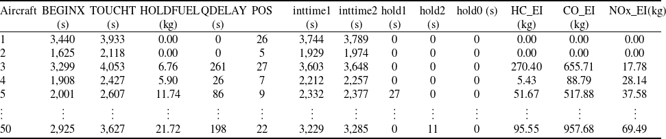
Beyond global performance indicators, the restricted MILP produces detailed aircraft-level outputs (Table 3), including start and take-off times (BEGINX, TOUCHT), queueing delays (QDELAY), final sequence position (POS), location-specific holds (hold0/1/2) and associated emissions (HC, CO, NOx). These fields are directly compatible with the information needs of pre-tactical tools such as a DMAN operating within the airport collaborative decision making (A-CDM) framework. Given a set of off-block intentions, the model can be used to generate target take-off times (TTOT) and target start-up approval times (TSAT) that are both fuel-efficient and CPS-compliant, and that can be refreshed in pre-tactical time frame on the order of tens of minutes as conditions change [59].
Sample aircraft-level outputs from the restricted-MILP evaluator for a single optimised sequence

Table 3 Long description
The table presents detailed aircraft-level outputs from a restricted Mixed-Integer Linear Programming (MILP) evaluator for a single optimized sequence. It includes columns for start time (BEGINX), take-off time (TOUCHT), hold fuel (HOLDFUEL), queueing delay (QDELAY), final sequence position (POS), intermediate times (inttime1, inttime2), hold times (hold1, hold2, hold0), and emissions (HC_EI, CO_EI, NOx_EI). The table has 50 rows and 13 columns. Each row represents an aircraft, with values for each of the mentioned parameters. Notable trends include varying hold fuel and emissions across different aircraft, with some aircraft having significant queueing delays and hold times. The emissions data shows a range of values for hydrocarbons (HC_EI), carbon monoxide (CO_EI), and nitrogen oxides (NOx_EI), indicating the environmental impact of each aircraft's operations.
Implications for air traffic controllers (ATCos). For controllers, the main value of the framework lies in its ability to translate a complex optimisation into a small number of interpretable and schedulable moves.
-
• Where and when to delay aircraft: Explicit hold durations at named locations (e.g. hold1, hold2) allow ATCos to see where delay is absorbed and to verify that separation standards are met without overusing runway-adjacent holding points.
-
• Position shifting within CPS limits: The POS and CPS structure make it clear which flights have been advanced or deferred relative to FCFS and by how many positions, supporting fairness and equity discussions with airlines.
-
• Final sequence validation: Because every candidate is evaluated by a full MILP, controllers know that the proposed ordering is globally feasible with respect to separation and taxi network interactions, rather than being the result of a local repair heuristic.
These properties enable the design of DSS interfaces where ATCos can inspect the proposed queue, highlight individual swaps or inserts and immediately see the effect on fuel, delay and emissions, instead of being asked to trust a purely numerical ‘optimal’ solution. The conflict-visualisation work in Ref. [Reference Dönmez60] demonstrates how similar outputs from the same Antalya model can be mapped onto taxiway layouts and runway timelines, further reinforcing situational awareness.
Implications for airport and airline operators. For airport and airline stakeholders, the aircraft-level outputs support both tactical decisions and longer-term performance monitoring.
-
• Hold-fuel management and costs: HOLDFUEL values quantify the additional fuel burned due to ground holding and queueing, enabling airlines to estimate cost impacts and airports to evaluate the benefit of improved sequencing policies.
-
• Emission monitoring: HC, CO and NOx emission estimates along the taxi-out phase provide a basis for environmental reporting, sustainability key performance indicators (KPIs) and scenario comparisons (e.g. evaluating alternative cost-weightings between fuel and delay).
-
• Delay and bottleneck analysis: QDELAY and POS information can be aggregated over time to identify recurrent choke points in the ground operation and to inform infrastructure or procedural investments.
Overall, the proposed matheuristic approach provides numerically precise, operationally explainable schedules that can feed directly into decision-support tools for ATCos, airport operators and airlines. It thereby bridges the long-standing gap between exact but opaque optimisation and fast but oversimplified heuristic rules.
8.0 Future work
The present work focuses on departure scheduling for a single runway and a one-hour traffic sample calibrated for Antalya Airport. Several extensions are worth pursuing to increase realism and operational impact.
Antalya typically operates its parallel runways in a segregated fashion during busy periods, with departures and arrivals predominantly assigned to different runways; hence, arrivals do not interleave with the departure stream optimised in this study (see Fig. 31 in Ref. [Reference Dönmez61]). When mixed-mode operations are required in future work, the existing formulation can be extended by treating arrivals as exogenous runway-blocking windows: for each landing
 $\ell $
with touchdown time
 ${\tau _\ell }$
, we reserve an interval
 $\left[ {{\tau _\ell } - {\delta ^{{\rm{in}}}},{\tau _\ell } + {\delta ^{{\rm{out}}}}} \right]$
and constrain departure touchdown times to lie outside these windows via standard disjunctive (big-
 $M$
) constraints. This preserves CPS and wake-separation rules while explicitly accounting for arrival interference. A natural next step is to validate such a mixed-mode extension on busier hubs where arrival–departure interleaving is unavoidable.
A key limitation of the current study is the lack of access to proprietary surface-movement data for Antalya Airport, which prevents a direct comparison between optimised sequences and realised departure streams, taxi-out profiles and fuel consumption. Securing access to A-CDM logs, advanced surface movement guidance and control system (A-SMGCS) trajectories or automatic dependent surveillance–broadcast (ADS-B) data would enable (i) statistical calibration of taxi-time and fuel models, (ii) retrospective replay of historical traffic under alternative sequencing policies and (iii) out-of-sample validation of the matheuristic recommendations against real operational outcomes.
In this paper, all metaheuristic variants are evaluated using the same restricted MILP; ‘pure’ TS/SA/MACO/BFOA configurations without the MILP have not been reported. This is intentional: our comparison principle is that every candidate order should be scored by the same feasibility and timing engine so that all methods are assessed under an identical, operationally valid objective. Removing the MILP would require designing an alternative evaluator – typically a deterministic forward-propagation model plus conflict-repair rules – which would change the scoring function and undermine strict comparability with FCFS and the MILP-backed matheuristics. A fair MILP-free benchmark would need (i) a precisely specified propagation model, (ii) explicit repair policies for separation violations, (iii) identical wall-clock budgets and (iv) additional metrics such as feasibility rate and violation duration. Developing such baselines, and combining the current restricted-MILP approach with other metaheuristics (e.g. genetic algorithms or large neighbourhood search), is a promising avenue for future research.
While we reported a first time-limit sensitivity experiment, a more systematic analysis of model parameters remains to be done. Future work should examine the effect of CPS bounds, wake-separation standards, emission cost weights and uncertainty in ETD/taxi-time predictions on both solution quality and algorithm behaviour. Scenario-based or stochastic variants of the restricted MILP could be used to hedge against variability in demand or surface conditions. Similarly, multi-objective formulations that trade off fuel, delay, fairness (CPS) and emissions could be explored, with the metaheuristics operating on weighted sums or Pareto-based dominance criteria.
Finally, the current framework optimises static one-hour snapshots. In real operations, departure streams evolve as new flight information arrives, aircraft miss slots or runway configuration changes. Embedding the restricted-MILP matheuristics in a rolling-horizon controller that periodically re-optimises the sequence while preserving stability (e.g. through additional position-locking constraints) would bring the method closer to a deployable DMAN module. Coupling this with the explainable move-by-move outputs developed in this paper would enable human-in-the-loop controllers to monitor and selectively apply recommended adjustments in real time.
In summary, the proposed matheuristic framework offers a balanced compromise between exactness, computational tractability and operational explainability for departure sequencing. Building on these foundations through richer data, extended models and online control architectures has the potential to deliver more efficient, sustainable and resilient airport operations.
Acknowledgment
This research received no specific grant from any funding agency in the public, commercial or not-for-profit sectors.
Declaration of generative AI and AI-assisted technologies in the writing process
During the preparation of this work the author(s) used ChatGPT in order to improve language and readability, with caution. After using this tool/service, the author(s) reviewed and edited the content as needed and take(s) full responsibility for the content of the publication.


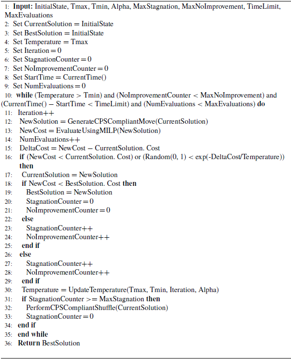
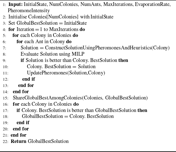
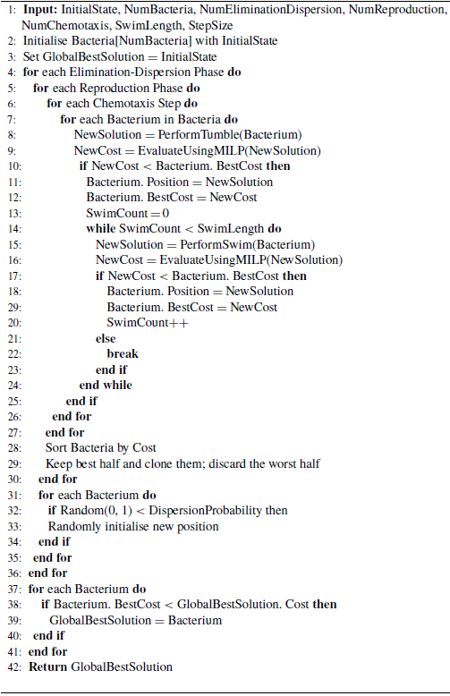
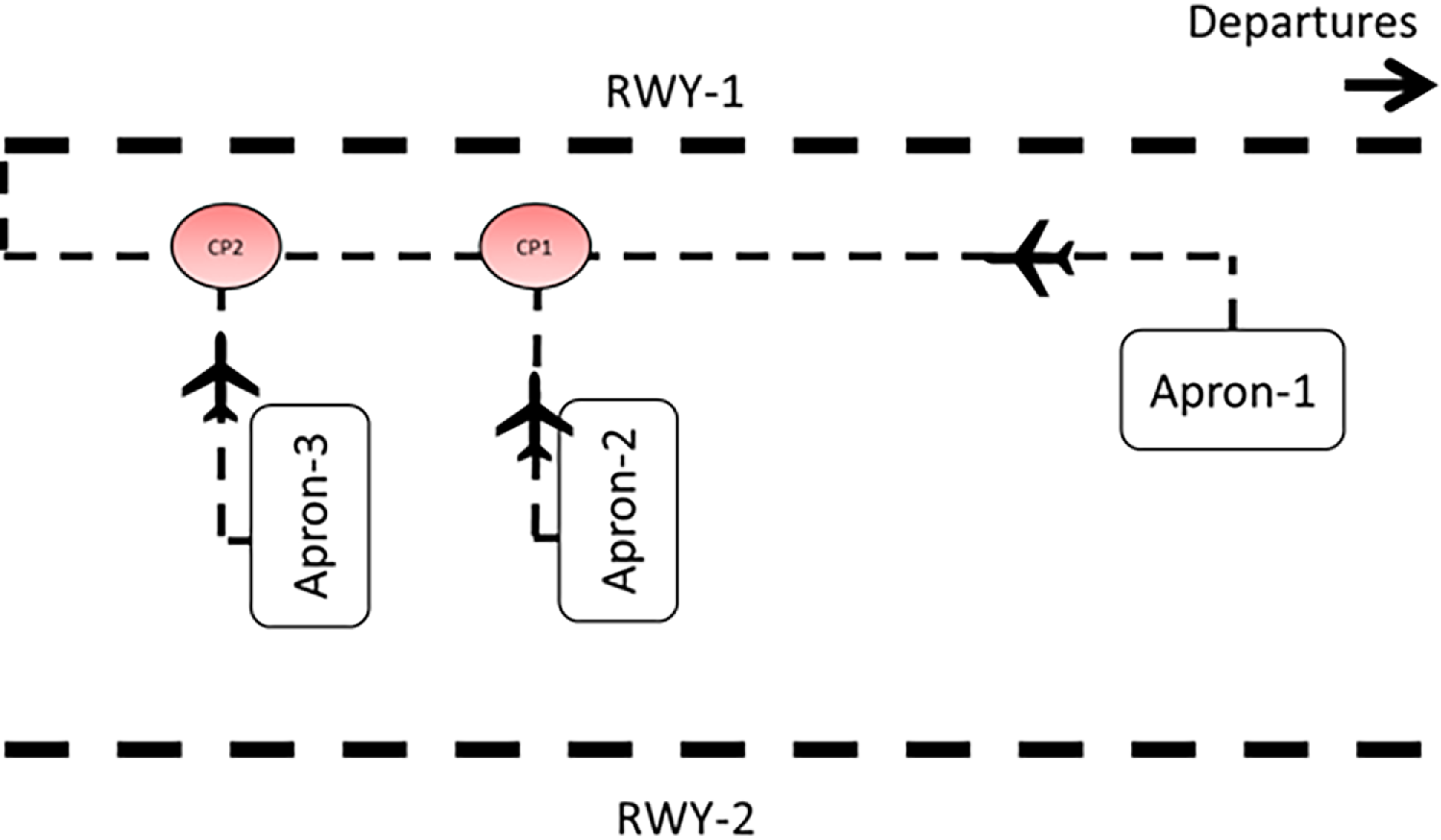



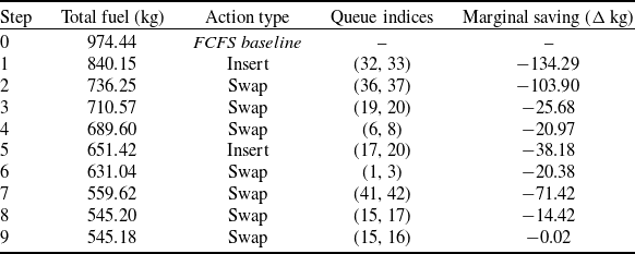

 974.44
 520.10