1 Introduction
Stratified plane Couette flow is bounded by two horizontal walls moving in opposite directions with a constant velocity. The fluid density at each wall is held at a constant value with a lower density at the upper wall, resulting in a stably stratified system. Stratified plane Couette flow is one of several canonical geometries used to investigate the dynamics of stratified shear flows. Much of the research on stratified plane Couette flow has focused on transition and coherent structures (Deusebio, Caulfield & Taylor Reference Deusebio, Caulfield and Taylor2015; Eaves & Caulfield Reference Eaves and Caulfield2015), turbulent characteristics (García-Villalba, Azagra & Uhlmann Reference García-Villalba, Azagra, Uhlmann and Nagel2011a ) and diapycnal mixing (Caulfield, Tang & Plasting Reference Caulfield, Tang and Plasting2004; Tang, Caulfield & Kerswell Reference Tang, Caulfield and Kerswell2009; García-Villalba, Azagra & Uhlmann Reference García-Villalba, Azagra and Uhlmann2011b ; Deusebio et al. Reference Deusebio, Caulfield and Taylor2015; Scotti Reference Scotti2015). In this paper, we consider the dynamical properties of turbulent stratified plane Couette flow. Our consideration has three main themes: (i) the effects of varying Prandtl number; (ii) the applicability of Monin–Obukhov similarity theory; and (iii) the parameterization of diapycnal mixing in stratified plane Couette flows. Each of the themes is associated with key open questions in the literature.
A stratified plane Couette flow can be characterized by three external parameters: the bulk Reynolds number
 $Re$
; the bulk Richardson number
 $Ri$
; and the Prandtl (Schmidt) number
 $Pr\equiv \unicode[STIX]{x1D708}/\unicode[STIX]{x1D705}$
(or
 $Sc$
), where
 $\unicode[STIX]{x1D705}$
is the scalar diffusivity and
 $\unicode[STIX]{x1D708}$
is the kinematic viscosity. While existing stratified plane Couette flow research spans a considerable range of
 $Re$
and
 $Ri$
, the
 $Pr$
(or equivalently
 $Sc$
) values examined have heretofore been limited to order unity. On the other hand, there has been growing evidence indicating that
 $Pr$
(or
 $Sc$
) can indeed have some first-order effects on stratified shear flows. For example, the effects of
 $Pr$
on the characteristics of secondary instabilities and diapycnal mixing were reported by Salehipour, Peltier & Mashayek (Reference Salehipour, Peltier and Mashayek2015) through simulations of growing Kelvin–Helmholtz instabilities. Motivated by these observations, we aim to investigate the effects of variations in
 $Pr$
systematically in stratified plane Couette flows through direct numerical simulation (DNS), and this investigation constitutes the first theme of this paper.
Stratified plane Couette flows transfer momentum and heat fluxes across the upper and lower walls which provide shear and stratification to the system. In fully developed statistically stationary turbulent stratified plane Couette flows, which are the focus of the present study, the total momentum and active scalar fluxes are constant in the wall-normal (vertical) direction
 $y$
. The very fact that these fluxes are constant in
 $y$
contrasts stratified plane Couette flows with other wall-bounded flows, such as channel flows (Armenio & Sarkar Reference Armenio and Sarkar2002; García-Villalba & del Álamo Reference García-Villalba and del Álamo2011; Karimpour & Venayagamoorthy Reference Karimpour and Venayagamoorthy2014, Reference Karimpour and Venayagamoorthy2015), where the total momentum flux is maximized at the walls and zero at midchannel (see e.g. Armenio & Sarkar Reference Armenio and Sarkar2002). Turner (Reference Turner1973) argued that stably stratified flows may adjust to a tuned vertical flux from rearrangement of the mean flow and scalar profiles, and the turbulent characteristics in such generic constant-flux layers warrant further study.
For decades (see Foken Reference Foken2006 for a review), the Monin–Obukhov similarity theory has provided a powerful tool to characterize such constant-flux layers. More recently, Monin–Obukhov theory has also been used to interpret stratified turbulence characteristics in homogeneous shear flows (Chung & Matheou Reference Chung and Matheou2012). In the context of stratified plane Couette flows, Deusebio et al. (Reference Deusebio, Caulfield and Taylor2015) demonstrated the usefulness of Monin–Obukhov scaling by delineating the intermittency boundary in
 $(Re,Ri)$
parameter space at a single Prandtl number
 $Pr=0.7$
. The Obukhov length scale
 $$\begin{eqnarray}L\equiv \frac{u_{\unicode[STIX]{x1D70F}}^{3}}{k_{m}g\unicode[STIX]{x1D6FC}_{V}q_{w}},\end{eqnarray}$$
was found to be of dynamical significance in stratified plane Couette flows. Here,
 $u_{\unicode[STIX]{x1D70F}}$
is the friction velocity,
 $k_{m}$
is the von Kármán constant for momentum,
 $g$
is gravity,
 $\unicode[STIX]{x1D6FC}_{V}$
is the thermal expansion coefficient relating fluid temperature
 $\unicode[STIX]{x1D703}$
to density
 $\unicode[STIX]{x1D70C}$
via a linear equation of state
 $$\begin{eqnarray}\unicode[STIX]{x1D70C}=\unicode[STIX]{x1D70C}_{0}(1-\unicode[STIX]{x1D6FC}_{V}\unicode[STIX]{x1D703}),\end{eqnarray}$$
with
 $\unicode[STIX]{x1D70C}_{0}$
being the reference density and
 $q_{w}$
is the wall heat flux. The ratio of length scales,
 $$\begin{eqnarray}L^{+}\equiv \frac{L}{\unicode[STIX]{x1D6FF}_{\unicode[STIX]{x1D708}}},\end{eqnarray}$$
where
 $\unicode[STIX]{x1D6FF}_{\unicode[STIX]{x1D708}}\equiv \unicode[STIX]{x1D708}/u_{\unicode[STIX]{x1D70F}}$
is the near-wall viscous length scale, needs to be above approximately 200 for a stratified plane Couette (SPC) flow to stay fully turbulent, while when
 $L^{+}<200$
the flows become intermittent, i.e. laminar and turbulent flow patches coexist. This observation is consistent with Flores & Riley (Reference Flores and Riley2011) who reported similar behaviour in stably stratified boundary layers. Consistent with the
 $L^{+}$
criterion, Deusebio et al. (Reference Deusebio, Caulfield and Taylor2015) were not able to find fully developed turbulence (see their figure 18) in the SPC system for
 $Ri>0.2$
even for
 $Re$
up to 280 000, as the flow inevitably relaminarizes due to the strong buoyancy effects, although it is important to appreciate that the simulations had imposed periodicity in the streamwise and spanwise directions, and the extent of the computational domain may play a non-trivial role. Subsequently, Scotti & White (Reference Scotti and White2016) also used Monin–Obukhov similarity theory to consider, among other issues, the mixing properties of stratified plane Couette flow, but they restricted their attention to five simulations at relatively low
 $Ri\leqslant 0.1$
for
 $14\,250\leqslant Re\leqslant 55\,000$
, using our conventions, and the single value of
 $Pr=1$
, and so did not consider the parameter regime where this intermittency at high
 $Re$
for sufficiently high
 $Ri$
appears to arise.
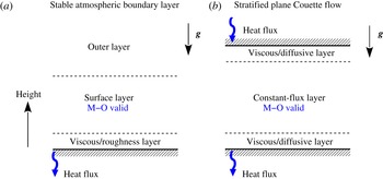
In this paper, we employ Monin–Obukhov similarity theory to formulate scalings for relevant stratified flow diagnostics in stratified plane Couette flows, which forms the second theme of the paper. It is important to contrast the behaviour of stratified plane Couette flows with the more geophysically realistic flow in a stable atmospheric boundary layer, where the flow is only wall bounded from below. In stable atmospheric boundary layers, Monin–Obukhov theory is only valid for the ‘weakly stable’ regime in the surface layer where the momentum and buoyancy fluxes do not vary with height, as shown in figure 1(a). Monin–Obukhov theory does not apply, for example, in the overlying outer layer, or in the ‘very stable’ regime where the constant-flux surface layer does not exist (see e.g. Mahrt Reference Mahrt2014). However, in the doubly bounded set-up of stratified plane Couette flows, as shown in figure 1(b), the momentum and buoyancy fluxes do not vary over height under the condition of statistical stationarity, and Monin–Obukhov theory is indeed expected to hold throughout the domain, crucially because the flow is wall bounded above and below, and so there is a
 $y$
-independent vertical flux through the domain.
One of the specific goals of the paper is to examine whether stratified plane Couette flow (or any stable constant-flux layer to which Monin–Obukhov scaling applies) supports the strongly stratified turbulence regime (Lilly Reference Lilly1983; Billant & Chomaz Reference Billant and Chomaz2001; Brethouwer et al.
Reference Brethouwer, Billant, Lindborg and Chomaz2007; Riley & Lindborg Reference Riley, Lindborg, Davidson, Kaneda and Sreenivasan2012), a regime which requires
 $Re_{b}\gg 1$
and
 $Fr_{h}\ll 1$
, where
 $Re_{b}$
is the buoyancy Reynolds number and
 $Fr_{h}$
is the horizontal turbulent Froude number.
 $Re_{b}$
and
 $Fr_{h}$
are defined as
 $$\begin{eqnarray}Re_{b}\equiv \frac{\unicode[STIX]{x1D700}}{\unicode[STIX]{x1D708}N^{2}}\quad \text{and}\quad Fr_{h}\equiv \frac{U^{\prime }}{N\ell _{h}},\end{eqnarray}$$
where
 $\unicode[STIX]{x1D700}$
is the dissipation rate,
 $N$
is the buoyancy frequency,
 $U^{\prime }$
is a characteristic turbulent horizontal velocity and
 $\ell _{h}$
is the horizontal integral scale of the turbulence. Such a strongly stratified regime can be reached numerically in homogeneous and stationary flows with body forcing (Brethouwer et al.
Reference Brethouwer, Billant, Lindborg and Chomaz2007; de Bruyn Kops Reference de Bruyn Kops2015), and in unforced non-stationary flows with specific initial conditions (Riley & de Bruyn Kops Reference Riley and de Bruyn Kops2003; Diamessis, Spedding & Domaradzki Reference Diamessis, Spedding and Domaradzki2011; Maffioli & Davidson Reference Maffioli and Davidson2015; Zhou Reference Zhou2015). However, the existence of the strongly stratified regime has not been reported in wall-bounded stratified flows (García-Villalba & del Álamo Reference García-Villalba and del Álamo2011; García-Villalba et al.
Reference García-Villalba, Azagra, Uhlmann and Nagel2011a
; Deusebio et al.
Reference Deusebio, Caulfield and Taylor2015). Whether this regime is realizable in such flows is a key issue that we investigate in this paper. As demonstrated in Scotti & White (Reference Scotti and White2016), Monin–Obukhov scaling allows the construction of an estimate for
 $Re_{b}$
, and so for flows exhibiting Monin–Obukhov scaling there is a convenient theoretical approach to consider the realizability of the strongly stratified regime.
Comparison of a ‘weakly stable’ atmospheric boundary layer (see e.g. Mahrt Reference Mahrt2014) and a stratified plane Couette flow. The heights of various layers are not drawn to scale.

Diapycnal mixing in stratified flows is a focal point of research (see the reviews of Linden (Reference Linden1979), Fernando (Reference Fernando1991), Peltier & Caulfield (Reference Peltier and Caulfield2003), Ivey, Winters & Koseff (Reference Ivey, Winters and Koseff2008)). Existing parameterizations of the diapycnal diffusivity
 $\unicode[STIX]{x1D705}_{t}$
, when normalized by the molecular viscosity
 $\unicode[STIX]{x1D708}$
, often involve
 $Re_{b}$
as a parameter (Shih et al.
Reference Shih, Koseff, Ivey and Ferziger2005; Bouffard & Boegman Reference Bouffard and Boegman2013), although it has been widely debated if
 $Re_{b}$
is the only parameter of relevance. For example, the additional effects of
 $Ri_{g}$
and
 $Pr$
have been highlighted by laboratory and numerical studies (Barry et al.
Reference Barry, Ivey, Winters and Imberger2001; Mater & Venayagamoorthy Reference Mater and Venayagamoorthy2014; Salehipour & Peltier Reference Salehipour and Peltier2015; Salehipour et al.
Reference Salehipour, Peltier and Mashayek2015; Maffioli, Brethouwer & Lindborg Reference Maffioli, Brethouwer and Lindborg2016; Scotti & White Reference Scotti and White2016) in parameterizing
 $\unicode[STIX]{x1D705}_{t}$
, where
 $Ri_{g}$
is the gradient Richardson number defined as
 $$\begin{eqnarray}Ri_{g}\equiv \frac{N^{2}}{S^{2}},\end{eqnarray}$$
with
 $S$
being an appropriate mean vertical shear. A recent study by Maffioli et al. (Reference Maffioli, Brethouwer and Lindborg2016) proposed an alternative scaling based upon the turbulent Froude number
 $Fr_{h}$
defined in (1.4). Stratified plane Couette flow is an effective test bed for these parameterizations, as the parameters
 $(Re_{b},Ri_{g},Pr,Fr_{h})$
can be varied readily by adjusting the external properties (such as wall velocity, density difference, viscosity, etc.) in simulations of stratified plane Couette flow. The final theme of this paper is, therefore, to characterize the diapycnal mixing due to stratified turbulence in stratified plane Couette flow at as large a range of
 $Ri_{g}$
,
 $Re_{b}$
and
 $Pr$
as possible and to identify the relevant parameters in determining the turbulent diffusivities in such flows.
In summary, the three main aims of this paper and the corresponding open questions are as follows.
-
(i) Prandtl number effects. For given values of
 $(Re,Ri)$
, how do the mean flow and temperature profiles depend on
$Pr$
? How do the wall fluxes of momentum and heat depend on
$Pr$
? How does the intermittency boundary in
$(Re,Ri)$
parameter space vary with
$Pr$
?
-
(ii) Similarity scaling. How well does Monin–Obukhov theory characterize fully developed stratified plane Couette flow? How do diagnosed quantities such as
$Ri_{g}$
,
$Re_{b}$
and
$Fr_{h}$
, arising as outputs of the simulations, relate to the wall fluxes? How do those diagnostics relate to each other? Is the strongly stratified regime accessible in stratified plane Couette flows? -
(iii) Mixing parameterization. How should one parameterize the turbulent diffusivities in stratified plane Couette flows? Which of the possible parameters
$(Re_{b},Ri_{g},Pr,Fr_{h})$
play a role in these flows? Are these parameters independent of each other?



To address these questions, the rest of the paper is structured as follows. In § 2 we describe our numerical simulations of stratified plane Couette flows. In § 3, we review Monin–Obukhov similarity theory and develop a mixing length model incorporating Monin–Obukhov theory at various Prandtl numbers and applying near-wall corrections (unlike the
 $Pr=1$
model presented in Scotti & White (Reference Scotti and White2016) not specifically focussed on stratified plane Couette flow), to predict the wall fluxes in stratified plane Couette flow as a function of external parameters
 $(Re,Ri,Pr)$
. In § 4 we present the Prandtl number effects in stratified plane Couette flows through the modification of the near-wall layer and thus the wall fluxes, and explore the implications of these effects for the intermittency boundary in the
 $(Re,Ri)$
plane. In § 5 we employ Monin–Obukhov similarity theory to characterize the turbulence in the channel gap interior and formulate scalings for various flow diagnostics. In § 6 we develop parameterizations for turbulent diffusivities in the channel gap interior and discuss the results in the context of Monin–Obukhov scalings presented in § 5 and existing parameterizations in the literature. In § 7 we provide some concluding remarks.
2 Numerical simulations
In this section we describe DNS of stratified plane Couette flows considered in this paper. These simulations follow closely those of Deusebio et al. (Reference Deusebio, Caulfield and Taylor2015) (hereinafter referred to as DCT). With a brief summary provided here, we refer the interested reader to DCT for further details on the formulation of the stratified plane Couette simulations. Full descriptions of the DNS algorithms can be found in Taylor (Reference Taylor2008) and Bewley (Reference Bewley2010).
Consider the velocity vector
 $\boldsymbol{u}=(u,v,w)$
in the coordinate system
 $(x,y,z)$
, where
 $x$
and
 $z$
are the periodic (horizontal) directions and
 $y$
the wall-normal (vertical) direction. Two non-slip solid walls, moving in opposite directions in the
 $x$
-direction at velocity
 $\pm U_{w}$
, are located at
 $y=\pm h$
respectively. The temperatures
 $\unicode[STIX]{x1D703}$
at the upper and lower walls are fixed at
 $\pm T_{w}$
respectively, resulting in a statically stable stratified system. We consider the incompressible Navier–Stokes equations under the Boussinesq approximation with a linear equation of state as given in (1.2):
 $$\begin{eqnarray}\displaystyle & \displaystyle \frac{\unicode[STIX]{x2202}\boldsymbol{u}}{\unicode[STIX]{x2202}t}+\boldsymbol{u}\boldsymbol{\cdot }\unicode[STIX]{x1D735}\boldsymbol{u}=-\frac{\unicode[STIX]{x1D735}p}{\unicode[STIX]{x1D70C}_{0}}+\unicode[STIX]{x1D708}\unicode[STIX]{x1D6FB}^{2}\boldsymbol{u}-\unicode[STIX]{x1D6FC}_{V}\unicode[STIX]{x1D703}\boldsymbol{g}, & \displaystyle\end{eqnarray}$$
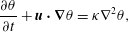 $$\begin{eqnarray}\displaystyle & \displaystyle \frac{\unicode[STIX]{x2202}\unicode[STIX]{x1D703}}{\unicode[STIX]{x2202}t}+\boldsymbol{u}\boldsymbol{\cdot }\unicode[STIX]{x1D735}\unicode[STIX]{x1D703}=\unicode[STIX]{x1D705}\unicode[STIX]{x1D6FB}^{2}\unicode[STIX]{x1D703}, & \displaystyle\end{eqnarray}$$
 $$\begin{eqnarray}\displaystyle & \displaystyle \unicode[STIX]{x1D735}\boldsymbol{\cdot }\boldsymbol{u}=0, & \displaystyle\end{eqnarray}$$
 $\unicode[STIX]{x1D708}$
and
 $\unicode[STIX]{x1D705}$
are the kinematic viscosity and thermal diffusivity respectively, and
 $\boldsymbol{g}\equiv -g\boldsymbol{e}_{y}$
represents gravity. (It is important to remember that the vertical axis in which gravity acts is denoted by
 $y$
as is conventional in engineering wall-bounded flow contexts, whereas in geophysical contexts this direction is often denoted by
 $z$
.)
Stratified plane Couette flows are characterized by three external parameters:
 $$\begin{eqnarray}Re\equiv \frac{U_{w}h}{\unicode[STIX]{x1D708}},\quad Ri\equiv \frac{\unicode[STIX]{x1D6FC}_{V}T_{w}gh}{U_{w}^{2}}\quad \text{and}\quad Pr\equiv \frac{\unicode[STIX]{x1D708}}{\unicode[STIX]{x1D705}}.\end{eqnarray}$$
We denote the mean velocity and temperature by
 $$\begin{eqnarray}U\equiv \langle u\rangle \quad \text{and}\quad \unicode[STIX]{x1D6E9}\equiv \langle \unicode[STIX]{x1D703}\rangle ,\end{eqnarray}$$
respectively, where
 $\langle \cdots \rangle$
represents horizontal averages over the statistically homogeneous
 $x$
–
 $z$
plane. The friction velocity
 $u_{\unicode[STIX]{x1D70F}}$
and temperature
 $\unicode[STIX]{x1D703}_{\unicode[STIX]{x1D70F}}$
are defined as
 $$\begin{eqnarray}u_{\unicode[STIX]{x1D70F}}^{2}\equiv \frac{\unicode[STIX]{x1D70F}_{w}}{\unicode[STIX]{x1D70C}_{0}}=\unicode[STIX]{x1D708}\left|\frac{\unicode[STIX]{x2202}U}{\unicode[STIX]{x2202}y}\right|_{y=\pm h}\quad \text{and}\quad \unicode[STIX]{x1D703}_{\unicode[STIX]{x1D70F}}\equiv \frac{q_{w}}{u_{\unicode[STIX]{x1D70F}}}\end{eqnarray}$$
respectively, where
 $\unicode[STIX]{x1D70F}_{w}\equiv \unicode[STIX]{x1D70C}_{0}u_{\unicode[STIX]{x1D70F}}^{2}$
is the wall shear stress and
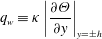 $$\begin{eqnarray}q_{w}\equiv \unicode[STIX]{x1D705}\left|\frac{\unicode[STIX]{x2202}\unicode[STIX]{x1D6E9}}{\unicode[STIX]{x2202}y}\right|_{y=\pm h}\end{eqnarray}$$
is the wall heat flux. The Obukhov length scale
 $L$
, defined in (1.1), is the only (up to a multiplicative constant) length scale that can be formed using
 $u_{\unicode[STIX]{x1D70F}}^{2}$
and
 $q_{w}$
, the wall momentum and heat fluxes, along with the buoyancy parameter
 $g\unicode[STIX]{x1D6FC}_{V}$
, where
 $\unicode[STIX]{x1D6FC}_{V}$
relates temperature to buoyancy via the linear equation of state (1.2). The friction velocity
 $u_{\unicode[STIX]{x1D70F}}$
can be used to form the friction Reynolds number
 $$\begin{eqnarray}Re_{\unicode[STIX]{x1D70F}}\equiv \frac{u_{\unicode[STIX]{x1D70F}}h}{\unicode[STIX]{x1D708}},\end{eqnarray}$$
and
 $q_{w}$
can be made dimensionless to form the Nusselt number
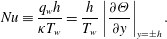 $$\begin{eqnarray}Nu\equiv \frac{q_{w}h}{\unicode[STIX]{x1D705}T_{w}}=\frac{h}{T_{w}}\left|\frac{\unicode[STIX]{x2202}\unicode[STIX]{x1D6E9}}{\unicode[STIX]{x2202}y}\right|_{y=\pm h}.\end{eqnarray}$$
 $Re_{\unicode[STIX]{x1D70F}}$
and
 $Nu$
are not known a priori, but are rather output parameters which vary with the external parameters
 $(Re,Ri,Pr)$
.
In order to investigate the flow properties as the external parameters vary in the three-dimensional parameter space
 $(Re,Ri,Pr)$
, we first revisit the existing simulations performed by DCT who focused on a fixed
 $Pr=0.7$
and varied
 $Re$
and
 $Ri$
extensively. A set of simulations performed by DCT at a wide range of
 $Re$
from 865 to 280 000 are reanalysed in the present study, and the parameters covered are listed in table 1. In addition, new simulations are performed at a fixed Reynolds number
 $Re=4250$
for various
 $Pr$
and
 $Ri$
. The
 $Re$
value in the new simulations is large enough to support fully developed turbulence at finite values of
 $Ri$
, (i.e. there is no observed spatial or temporal intermittency in the turbulent flow in this geometry) and yet the
 $Re$
value is small enough to allow, within available computing resources, a parametric study in the
 $(Ri,Pr)$
parameter space through DNS, which is one of the main aims of this paper.
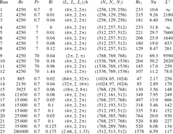
Summary of numerical simulations of stratified plane Couette flows. Simulations 1–12 are performed specifically for the present study with a fixed
 $Re=4250$
and varying
 $Pr$
and
 $Ri$
, and simulations 13–23 were first reported by Deusebio et al. (Reference Deusebio, Caulfield and Taylor2015) with a fixed
 $Pr=0.7$
and varying
 $Re$
and
 $Ri$
. The computational domains are of dimensions
 $(L_{x},L_{y},L_{z})$
, and the number of grid points in each direction is
 $(N_{x},N_{y},N_{z})$
respectively.
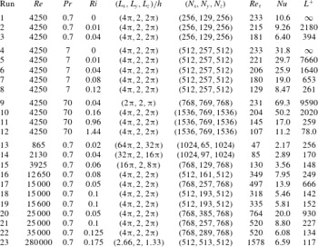
The input and output parameters of these simulations, both newly performed (simulations 1–12) and reanalysed from the work of DCT (simulations 13–23), are tabulated in table 1.
 $Pr$
values spanning two orders of magnitude, i.e.
 $Pr\in \{0.7,7,70\}$
, are considered in this paper. The choices of the first two
 $Pr$
values correspond to the geophysically relevant scenarios of heat (as the active scalar) in air (
 $Pr=0.7$
) and heat in water (
 $Pr=7$
) respectively. While the direct geophysical relevance of the third examined value of
 $Pr=70$
is not immediately apparent, it has been chosen as an intermediate value between 7 and 700, the latter of which corresponds to the relevant Schmidt number
 $Sc$
of salt in water. Simulation of flows with
 $Sc=700$
incurs prohibitive computational costs presently. The
 $Pr=70$
simulations are examined in an attempt to probe the extremely poorly conductive/diffusive regime expected to occur for
 $Sc=700$
.
In addition to the requirements to resolve the near-wall dynamics adequately, which dynamics was described by DCT, the elevated
 $Pr$
values impose their own requirement on the spatial resolution of the DNS, i.e. to resolve adequately the Batchelor scale of the scalar field
 $\ell _{B}$
(Batchelor Reference Batchelor1959), where
 $\ell _{B}$
is defined as
 $$\begin{eqnarray}\ell _{B}\equiv \frac{\unicode[STIX]{x1D702}}{Pr^{1/2}},\end{eqnarray}$$
and
 $\unicode[STIX]{x1D702}\equiv (\unicode[STIX]{x1D708}^{3}/\unicode[STIX]{x1D700})^{1/4}$
is the Kolmogorov scale. Equation (2.8) suggests that the grid resolution needs to be approximately tripled when
 $Pr$
is increased by one order of magnitude, given a fixed
 $\unicode[STIX]{x1D702}$
. In setting up our simulations, simulation 3 (which is replicated from DCT’s simulation 9 as tabulated in their table 1) with
 $(Re,Ri,Pr)=(4250,0.04,0.7)$
, is used as a reference. When
 $Pr$
is increased from 0.7 (as in DCT’s simulations) to 7 (as in our simulations 4–8), the resolution is only doubled. However, grid independence tests at
 $Pr=7$
employing a
 $384\times 193\times 384$
grid yield no significant differences in the turbulence statistics, suggesting that the resolutions of our
 $Pr=7$
simulations are sufficient. When
 $Pr$
is increased from 7 to 70 in simulations 9–12, the resolution is tripled, as required by (2.8).
In stratified plane Couette flow simulations, the size of the computational domain may affect the results when the flow is intermittent, as suggested by DCT. All but one of the new simulations (1–12) performed have horizontal domain dimensions of
 $(L_{x},L_{z})=(4\unicode[STIX]{x03C0}h,2\unicode[STIX]{x03C0}h)$
, following the baseline cases adopted by DCT (i.e. simulations 16–22). Due to the constraint of computational resources, however, the simulation of
 $(Ri,Pr)=(0.04,70)$
(simulation 9) is performed with the domain dimensions in
 $x$
and
 $z$
reduced to 50 % of the other simulations, while keeping the same spatial resolution. As reported by DCT, the turbulence statistics are not expected to be sensitive to the domain size if the flow is fully turbulent, which is the case of simulation 9. Throughout this paper, we focus on examining the turbulence characteristics during the statistically stationary phase of the simulations where key statistics such as
 $\text{d}U/\text{d}y$
,
 $\text{d}\unicode[STIX]{x1D6E9}/\text{d}y$
and
 $\unicode[STIX]{x1D700}$
are observed to have reached a steady state. The spatially averaged statistics may fluctuate weakly with time (see DCT’s figure 2(b) for example), and the statistics reported in the following are also time averaged over a time scale of no shorter than
 $5h/U_{w}$
, i.e. five advective time units, for the simulations with
 $Pr=70$
. For the simulations with
 $Pr=0.7$
and 7, the time-averaging window is typically longer than
 $50h/U_{w}$
.
3 First-order closure model
Key quantities in describing stratified plane Couette flows in the framework of Monin–Obukhov similarity theory are the momentum flux
 $u_{\unicode[STIX]{x1D70F}}^{2}$
and wall heat flux
 $q_{w}$
which are directly linked to the wall gradients via (2.4) and (2.5). It is thus desirable to develop a model to predict the fluxes for varying external parameters. DCT proposed such a model applying Monin–Obukhov theory to the Reynolds-averaged Navier–Stokes equations. However, the model only applied to a single Prandtl number (
 $Pr=0.7$
). A refined version of the model, which now uses a mixing length formulation to provide a first-order closure for the turbulent fluxes as a function of mean local gradients, is described here. The mixing length specifications are consistent with Monin–Obukhov theory, and near-wall corrections through damping functions (van Driest Reference van Driest1956; Pope Reference Pope2000) ensure the reliable presentation of the effects of
 $Pr$
on the wall fluxes.
3.1 Model formulation
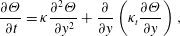
In order to obtain the vertical profiles of mean velocity and temperature in fully developed turbulent stratified plane Couette flow, we integrate the following set of equations of
 $U$
and
 $\unicode[STIX]{x1D6E9}$
in time (using the laminar profiles as initial conditions) until reaching a steady state:
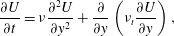 $$\begin{eqnarray}\displaystyle & \displaystyle \frac{\unicode[STIX]{x2202}U}{\unicode[STIX]{x2202}t}=\unicode[STIX]{x1D708}\frac{\unicode[STIX]{x2202}^{2}U}{\unicode[STIX]{x2202}y^{2}}+\frac{\unicode[STIX]{x2202}}{\unicode[STIX]{x2202}y}\left(\unicode[STIX]{x1D708}_{t}\frac{\unicode[STIX]{x2202}U}{\unicode[STIX]{x2202}y}\right), & \displaystyle\end{eqnarray}$$
 $$\begin{eqnarray}\displaystyle & \displaystyle \frac{\unicode[STIX]{x2202}\unicode[STIX]{x1D6E9}}{\unicode[STIX]{x2202}t}=\unicode[STIX]{x1D705}\frac{\unicode[STIX]{x2202}^{2}\unicode[STIX]{x1D6E9}}{\unicode[STIX]{x2202}y^{2}}+\frac{\unicode[STIX]{x2202}}{\unicode[STIX]{x2202}y}\left(\unicode[STIX]{x1D705}_{t}\frac{\unicode[STIX]{x2202}\unicode[STIX]{x1D6E9}}{\unicode[STIX]{x2202}y}\right), & \displaystyle\end{eqnarray}$$
where
 $\unicode[STIX]{x1D708}_{t}$
and
 $\unicode[STIX]{x1D705}_{t}$
are the turbulent (eddy) viscosity and diffusivity respectively.
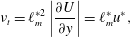
The closure for
 $\unicode[STIX]{x1D708}_{t}$
in the Reynolds-averaged momentum equation (3.1) can be obtained by specifying a mixing length (see e.g. Pope Reference Pope2000):
 $$\begin{eqnarray}\unicode[STIX]{x1D708}_{t}=\ell _{m}^{\ast 2}\left|\frac{\unicode[STIX]{x2202}U}{\unicode[STIX]{x2202}y}\right|=\ell _{m}^{\ast }u^{\ast },\end{eqnarray}$$
where
 $\ell _{m}^{\ast }$
is the mixing length for momentum and the fluctuation velocity
 $$\begin{eqnarray}u^{\ast }=\ell _{m}^{\ast }\left|\frac{\unicode[STIX]{x2202}U}{\unicode[STIX]{x2202}y}\right|.\end{eqnarray}$$
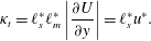
Similarly, the turbulent flux of scalar in (3.2) can be modelled as
 $$\begin{eqnarray}-\langle v^{\prime }\unicode[STIX]{x1D703}^{\prime }\rangle =\unicode[STIX]{x1D705}_{t}\frac{\unicode[STIX]{x2202}\unicode[STIX]{x1D6E9}}{\unicode[STIX]{x2202}y}=u^{\ast }\unicode[STIX]{x1D703}^{\ast }=\ell _{m}^{\ast }\left|\frac{\unicode[STIX]{x2202}U}{\unicode[STIX]{x2202}y}\right|\ell _{s}^{\ast }\frac{\unicode[STIX]{x2202}\unicode[STIX]{x1D6E9}}{\unicode[STIX]{x2202}y},\end{eqnarray}$$
where
 $\ell _{s}^{\ast }$
is the scalar mixing length, and it follows that
 $$\begin{eqnarray}\unicode[STIX]{x1D705}_{t}=\ell _{s}^{\ast }\ell _{m}^{\ast }\left|\frac{\unicode[STIX]{x2202}U}{\unicode[STIX]{x2202}y}\right|=\ell _{s}^{\ast }u^{\ast }.\end{eqnarray}$$
It remains to specify the two mixing lengths
 $\ell _{m}^{\ast }$
and
 $\ell _{s}^{\ast }$
.
To do this, we start by considering unstratified flows, i.e.
 $L\rightarrow \infty$
. We define
 $y_{w}$
as the wall-normal (vertical) distance to the closer wall, i.e.
 $y_{w}\equiv \min (h-y,h+y)$
. The length
 $y_{w}$
can be normalized in wall units as
 $y^{+}\equiv y_{w}/(\unicode[STIX]{x1D708}/u_{\unicode[STIX]{x1D70F}})$
. The ‘law of the wall’ of unstratified wall-bounded flows (see e.g. Bradshaw & Huang Reference Bradshaw and Huang1995) prescribes the wall-normal gradients of
 $U$
and
 $\unicode[STIX]{x1D6E9}$
in the log-law region, i.e.
 $y^{+}>30$
(Pope Reference Pope2000), as
 $$\begin{eqnarray}\frac{\unicode[STIX]{x2202}U}{\unicode[STIX]{x2202}y}=\frac{u_{\unicode[STIX]{x1D70F}}}{k_{m}y_{w}}\quad \text{and}\quad \frac{\unicode[STIX]{x2202}\unicode[STIX]{x1D6E9}}{\unicode[STIX]{x2202}y}=\frac{\unicode[STIX]{x1D703}_{\unicode[STIX]{x1D70F}}}{k_{s}y_{w}}=\frac{\unicode[STIX]{x1D703}_{\unicode[STIX]{x1D70F}}\hat{Pr}_{t}}{k_{m}y_{w}},\end{eqnarray}$$
where
 $k_{m}$
and
 $k_{s}$
are the von Kármán constants for momentum and scalar respectively, and
 $\hat{Pr}_{t}=k_{m}/k_{s}$
is a turbulent Prandtl number which applies for the log-law region. With
 $$\begin{eqnarray}u_{\unicode[STIX]{x1D70F}}^{2}\cong \unicode[STIX]{x1D708}_{t}\left|\frac{\unicode[STIX]{x2202}U}{\unicode[STIX]{x2202}y}\right|\quad \text{and}\quad q_{w}=\unicode[STIX]{x1D703}_{\unicode[STIX]{x1D70F}}u_{\unicode[STIX]{x1D70F}}\cong \unicode[STIX]{x1D705}_{t}\left|\frac{\unicode[STIX]{x2202}\unicode[STIX]{x1D6E9}}{\unicode[STIX]{x2202}y}\right|,\end{eqnarray}$$
in the log-law region and following the model prescriptions in (3.3) and (3.6), the mixing lengths
 $\ell _{m}^{\ast }$
and
 $\ell _{s}^{\ast }$
corresponding to (3.7) read
 $$\begin{eqnarray}\ell _{m}^{\ast }=k_{m}y_{w}\quad \text{and}\quad \ell _{s}^{\ast }=k_{s}y_{w}=\ell _{m}^{\ast }\hat{Pr}_{t}^{-1}.\end{eqnarray}$$
As a result, the velocity scale
 $u^{\ast }$
in (3.3) and (3.6) can be specified as
 $$\begin{eqnarray}u^{\ast }=u_{\unicode[STIX]{x1D70F}}.\end{eqnarray}$$
When the fluid is stratified, Monin–Obukhov similarity theory prescribes the vertical gradients of
 $U$
and
 $\unicode[STIX]{x1D6E9}$
as
 $$\begin{eqnarray}\frac{\unicode[STIX]{x2202}U}{\unicode[STIX]{x2202}y}=\frac{u_{\unicode[STIX]{x1D70F}}}{k_{m}y_{w}}\unicode[STIX]{x1D6F7}_{m}(\unicode[STIX]{x1D709})\quad \text{and}\quad \frac{\unicode[STIX]{x2202}\unicode[STIX]{x1D6E9}}{\unicode[STIX]{x2202}y}=\frac{\unicode[STIX]{x1D703}_{\unicode[STIX]{x1D70F}}}{k_{s}y_{w}}\unicode[STIX]{x1D6F7}_{s}(\unicode[STIX]{x1D709}).\end{eqnarray}$$
In these expressions,
 $\unicode[STIX]{x1D6F7}_{m}$
and
 $\unicode[STIX]{x1D6F7}_{s}$
are Monin–Obukhov functions which are linear in the non-dimensional variable
 $\unicode[STIX]{x1D709}\equiv y_{w}/L$
for stable stratification:
 $$\begin{eqnarray}\unicode[STIX]{x1D6F7}_{m}(\unicode[STIX]{x1D709})=1+\unicode[STIX]{x1D6FD}_{m}\unicode[STIX]{x1D709}\quad \text{and}\quad \unicode[STIX]{x1D6F7}_{s}(\unicode[STIX]{x1D709})=1+\unicode[STIX]{x1D6FD}_{s}\unicode[STIX]{x1D709}.\end{eqnarray}$$
Here we take
 $k_{m}=0.41$
and
 $k_{s}=0.48$
following Bradshaw & Huang (Reference Bradshaw and Huang1995). The choice of
 $\unicode[STIX]{x1D6FD}_{m}=4.8$
follows the recommendation of Wyngaard (Reference Wyngaard2010) and
 $\unicode[STIX]{x1D6FD}_{s}=5.6$
is used following the specific choice of
 $k_{m}$
and
 $k_{s}$
. These model constants are determined empirically using field observations of stable atmospheric boundary layers, and their values can exhibit some uncertainties (see Foken Reference Foken2006 for a review). The form of the similarity functions may also require additional corrections in order to match the field situations (see e.g. Tastula et al.
Reference Tastula, Galperin, Sukoriansky, Luhar and Anderson2015), such as varying fluxes with height. In the idealized situation considered here, where the entire flow between the walls is a constant-flux layer by construction, we use the classical canonical forms of Monin–Obukhov functions described in (3.12) for clarity and simplicity.
The mixing length formulation corresponding to Monin–Obukhov theory becomes
 $$\begin{eqnarray}\ell _{m}^{\ast }=k_{m}y_{w}\unicode[STIX]{x1D6F7}_{m}^{-1}(\unicode[STIX]{x1D709})\quad \text{and}\quad \ell _{s}^{\ast }=k_{s}y_{w}\unicode[STIX]{x1D6F7}_{s}^{-1}(\unicode[STIX]{x1D709}).\end{eqnarray}$$
Taking
 $\unicode[STIX]{x1D709}\rightarrow 0$
in (3.13), one recovers the unstratified formulation (3.9). Since
 $\ell _{m}^{\ast }$
and
 $\ell _{s}^{\ast }$
are specified in (3.13) in very similar ways, the ratio
 $\ell _{m}^{\ast }/\ell _{s}^{\ast }$
is expected to be of order unity.
3.2 The near-wall layer
Here we focus on the viscous wall region, i.e.
 $y^{+}<50$
(Pope Reference Pope2000), where the (molecular) Prandtl number
 $Pr$
plays a critical role. The mean velocity and temperature differences relative to the closer wall can be written in wall units as
 $$\begin{eqnarray}U^{+}=\frac{\min (U+U_{w},U_{w}-U)}{u_{\unicode[STIX]{x1D70F}}}\quad \text{and}\quad \unicode[STIX]{x1D6E9}^{+}=\frac{\min (\unicode[STIX]{x1D6E9}+T_{w},T_{w}-\unicode[STIX]{x1D6E9})}{\unicode[STIX]{x1D703}_{\unicode[STIX]{x1D70F}}},\end{eqnarray}$$
where the velocity and temperature at the upper and lower walls are fixed at
 $\pm U_{w}$
and
 $\pm T_{w}$
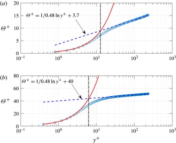
, respectively. In the viscous/conductive sublayer near the wall (as shown in figure 2 for
 $\unicode[STIX]{x1D6E9}^{+}$
),
 $$\begin{eqnarray}U^{+}=y^{+}\quad \text{and}\quad \unicode[STIX]{x1D6E9}^{+}=y^{+}Pr.\end{eqnarray}$$
As
 $y^{+}$
increases, the viscous/conductive sublayer transitions into the log-law region for which the mean profiles can be obtained by integrating (3.7) to yield
 $$\begin{eqnarray}U^{+}=\frac{1}{k_{m}}\ln y^{+}+C_{m}\quad \text{and}\quad \unicode[STIX]{x1D6E9}^{+}=\frac{1}{k_{s}}\ln y^{+}+C_{s}=\frac{\hat{Pr}_{t}}{k_{m}}\ln y^{+}+C_{s}.\end{eqnarray}$$
DNS of stratified plane Couette flows recover such behaviour in the near-wall region, as shown in figure 2. Unlike
 $C_{m}$
which is a constant (we take
 $C_{m}=5.0$
following Bradshaw & Huang (Reference Bradshaw and Huang1995)),
 $C_{s}$
is thought to be a function of
 $Pr$
, e.g. following Schlichting & Gersten (Reference Schlichting and Gersten2003),
 $$\begin{eqnarray}C_{s}=13.7Pr^{2/3}-7.5,\end{eqnarray}$$
or following Davidson (Reference Davidson2004),
 $$\begin{eqnarray}C_{s}=1.67(3Pr^{1/3}-1)^{2}.\end{eqnarray}$$
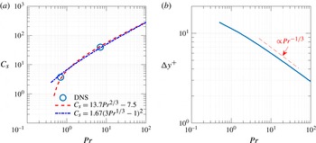
Figure 2 confirms such an effect of
 $Pr$
on the log-law layer. The empirical estimates of
 $C_{s}$
as a function of
 $Pr$
, i.e. (3.17) and (3.18), agree well with DNS, as shown in figure 3.
Normalized temperature difference from the wall value,
 $\unicode[STIX]{x1D6E9}^{+}$
as defined in (3.14), plotted as a function of normalized wall distance
 $y^{+}$
. (a)
 $Pr=0.7,Ri=0$
(simulation 1); (b)
 $Pr=7,Ri=0$
(simulation 4). Circles show DNS data; the conductive law (3.15) is plotted with a solid line; the logarithmic law (3.16) in which the additive constant
 $C_{s}$
varies with
 $Pr$
, is plotted with a dashed line; and the dot-dashed line shows the location of
 $y^{+}=\unicode[STIX]{x0394}y^{+}$
, where
 $\unicode[STIX]{x0394}y^{+}$
marks the characteristic height of the conductive sublayer as defined in (3.19).

The value of
 $C_{s}$
effectively determines the height of the conductive sublayer which can be measured by
 $\unicode[STIX]{x0394}y^{+}$
(as marked with vertical dot-dashed lines in figure 2), the intersect of the conductive law (3.15) and the log law (3.16), i.e.
 $$\begin{eqnarray}\unicode[STIX]{x0394}y^{+}Pr=\frac{1}{k_{s}}\ln \unicode[STIX]{x0394}y^{+}+C_{s}(Pr).\end{eqnarray}$$
The quantity
 $\unicode[STIX]{x0394}y^{+}$
is observed to decrease with
 $Pr$
(see figures 2 and 3), and, in particular, for
 $Pr\gg 1$
(Davidson Reference Davidson2004),
 $$\begin{eqnarray}\unicode[STIX]{x0394}y^{+}\propto Pr^{-1/3}.\end{eqnarray}$$
With (3.15), the temperature difference across the conductive sublayer, i.e.
 $$\begin{eqnarray}\unicode[STIX]{x0394}\unicode[STIX]{x1D6E9}^{+}\sim Pr\unicode[STIX]{x0394}y^{+}\propto Pr^{2/3},\end{eqnarray}$$
varies strongly with
 $Pr$
.
Effect of
 $Pr$
on the near-wall layer. (a) Variation with
 $Pr$
of the additive constant
 $C_{s}$
in the log law for scalar (3.16) as determined by simulations 1 and 4 of stratified plane Couette flows and empirical relations (3.17) and (3.18). (b) The height of the conductive sublayer
 $\unicode[STIX]{x0394}y^{+}$
as a function of
 $Pr$
.
 $\unicode[STIX]{x0394}y^{+}$
values obtained by solving (3.19) and (3.17) are plotted with a solid line, while the dashed line shows the scaling
 $\unicode[STIX]{x0394}y^{+}\propto Pr^{-1/3}$
.

It is thus shown that
 $Pr$
has a significant effect on the near-wall structure of the mean scalar field. A thinner conductive layer is expected at higher values of
 $Pr$
, as suggested by (3.20). Moreover, as the temperature gradients (in wall units) are sharper at a larger
 $Pr$
, as quantified by (3.15), the temperature jump across the conductive sublayer increases with
 $Pr$
, as quantified by (3.21). This generic behaviour of the ‘law of the wall’ for varying
 $Pr$
has implications for the overall temperature profile across the channel gap in stratified plane Couette flows, as we discuss in detail in § 4.
3.3 Damping functions
To complete the mixing length specifications by taking into account the near-wall layer and the effect of
 $Pr$
mentioned above, one can apply the van Driest damping functions (van Driest Reference van Driest1956) to the mixing lengths in (3.13). This near-wall correction improves the modelling of the turbulent fluxes in terms of their dependence on
 $y_{w}$
in the viscous/conductive sublayer (Pope Reference Pope2000). The momentum mixing length is corrected by the damping function
 $\text{D}_{m}(y^{+})$
to become
 $$\begin{eqnarray}\ell _{m}^{\ast }=k_{m}y_{w}\unicode[STIX]{x1D6F7}_{m}^{-1}(\unicode[STIX]{x1D709})\text{D}_{m}(y^{+})=k_{m}y_{w}\unicode[STIX]{x1D6F7}_{m}^{-1}(\unicode[STIX]{x1D709})[1-\exp (-y^{+}/A_{m}^{+})],\end{eqnarray}$$
where the van Driest constant for momentum
 $A_{m}^{+}$
is set to be 26 (van Driest Reference van Driest1956; Pope Reference Pope2000).
Similarly, the scalar mixing length becomes
 $$\begin{eqnarray}\ell _{s}^{\ast }=k_{s}y_{w}\unicode[STIX]{x1D6F7}_{s}^{-1}(\unicode[STIX]{x1D709})\text{D}_{s}(y^{+})=k_{s}y_{w}\unicode[STIX]{x1D6F7}_{s}^{-1}(\unicode[STIX]{x1D709})[1-\exp (-Pr^{-1}y^{+}/A_{s}^{+})],\end{eqnarray}$$
where the constant
 $A_{s}^{+}$
is inherently related to the
 $Pr$
-dependent additive constant
 $C_{s}$
in (3.16) (Pope Reference Pope2000) and is thus also a function of
 $Pr$
.
As
 $y^{+}\rightarrow 0$
, the turbulent diffusivity
 $\unicode[STIX]{x1D705}_{t}$
in the conductive sublayer, following (3.23), scales as
 $$\begin{eqnarray}\unicode[STIX]{x1D705}_{t}=\ell _{s}^{\ast }u^{\ast }=\ell _{s}^{\ast }\ell _{m}^{\ast }\left|\frac{\text{d}U}{\text{d}y}\right|\sim k_{s}k_{m}\frac{y^{+4}}{A_{s}^{+}A_{m}^{+}}\frac{\unicode[STIX]{x1D708}}{Pr}\sim k_{s}k_{m}\frac{y^{+4}}{A_{s}^{+}A_{m}^{+}}\unicode[STIX]{x1D705}.\end{eqnarray}$$
Note that (3.24) does not yield the expected power law, i.e.
 $\unicode[STIX]{x1D705}_{t}\propto y^{3}$
, that describes the near-wall variation of
 $\unicode[STIX]{x1D705}_{t}$
, which is a shortcoming of the van Driest model (see Pope Reference Pope2000, p. 305). We use the standard van Driest model for its simplicity. More sophisticated near-wall treatments for large Prandtl (Schmidt) number can be found in e.g. van Reeuwijk & Hadžiabdić (Reference van Reeuwijk and Hadžiabdić2015). The inclusion of
 $Pr^{-1}$
in the scalar damping function
 $\text{D}_{s}(y^{+})$
in (3.23) is such that
 $\unicode[STIX]{x1D705}_{t}$
in the near-wall limit is proportional to the molecular diffusivity
 $\unicode[STIX]{x1D705}$
(rather than
 $\unicode[STIX]{x1D708}=\unicode[STIX]{x1D705}Pr$
).
The quantity
 $A_{s}^{+}$
is, by definition, a dimensionless wall distance below which the damping takes place. A natural choice for
 $A_{s}^{+}$
is to take
 $A_{s}^{+}\sim \unicode[STIX]{x0394}y^{+}$
where the latter is a characteristic height of the conductive sublayer as defined by (3.19). In this model, we take
 $A_{s}^{+}=0.65\unicode[STIX]{x0394}y^{+}$
. This results in
 $A_{s}^{+}$
values of
 $\{7.9,4.3,2.1\}$
respectively for
 $Pr\in \{0.7,7,70\}$
.
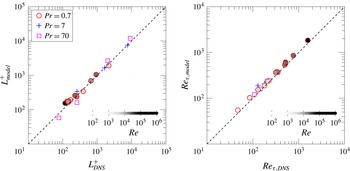
Comparison of the model prediction of
 $L^{+}$
and
 $Re_{\unicode[STIX]{x1D70F}}$
with DNS data from the present study and Deusebio et al. (Reference Deusebio, Caulfield and Taylor2015).
 $L_{model}^{+}$
and
 $Re_{\unicode[STIX]{x1D70F},model}$
are the results of the mixing length model as described in § 3;
 $L_{DNS}^{+}$
and
 $Re_{\unicode[STIX]{x1D70F},DNS}$
are the results of DNS which are tabulated in table 1. Varying Reynolds numbers are used in the simulations with
 $Pr=0.7$
(plotted with circles) and the fill colour is made darker for larger values of
 $Re$
.

3.4 Comparisons with DNS
This Monin–Obukhov mixing length model as described above can be implemented to produce predictions of wall fluxes
 $u_{\unicode[STIX]{x1D70F}}^{2}$
and
 $q_{w}$
and the dimensionless parameters defined in terms of the various fluxes, given the external parameters
 $Re$
,
 $Ri$
and
 $Pr$
. Figure 4 shows the comparisons between the model predictions of
 $L^{+}\equiv L/\unicode[STIX]{x1D6FF}_{\unicode[STIX]{x1D708}}$
and
 $Re_{\unicode[STIX]{x1D70F}}\equiv h/\unicode[STIX]{x1D6FF}_{\unicode[STIX]{x1D708}}$
(see definitions in (1.3) and (2.6) respectively) and DNS results at
 $Re=4250$
(the present study) and a (crucially) wider range of
 $Re$
values (Deusebio et al.
Reference Deusebio, Caulfield and Taylor2015) as listed in table 1. Given the considerable range of parameters, the agreement of the model predictions with DNS data is reasonable, with the
 $L_{2}$
norm of percentage relative errors being 16.4 % for
 $L^{+}$
and 13.9 % for
 $Re_{\unicode[STIX]{x1D70F}}$
over all simulations tested in figure 4. We believe that the model is thus validated and can be employed to produce an estimate of the wall fluxes given the (externally set)
 $(Re,Ri,Pr)$
parameters.
4 Effects of Prandtl number
In this section, we examine the DNS results focusing on the effects of the Prandtl number
 $Pr$
, which is the first main theme of this paper. In particular, we will address the three main questions already posed in the introduction: (i) how does
 $Pr$
modify the mean flow/temperature profiles; (ii) what do these modifications imply for the momentum and heat fluxes through the wall; and (iii) how does the intermittency boundary, delineated in the
 $(Re,Ri)$
space, vary with
 $Pr$
?
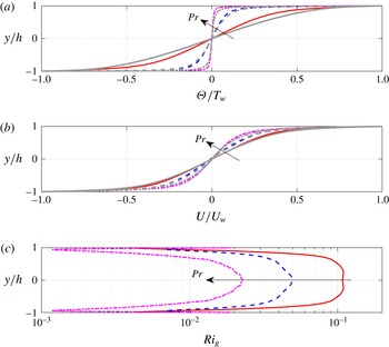
Figure 5 shows the effects of
 $Pr$
on the mean velocity (
 $U$
) and mean temperature (
 $\unicode[STIX]{x1D6E9}$
) profiles in the wall-normal
 $y$
-direction. At fixed values of
 $(Re,Ri)=(4250,0.04)$
, the mean temperature gradient
 $\text{d}\unicode[STIX]{x1D6E9}/\text{d}y$
(plotted in figure 5
a) sharpens significantly in the near-wall region, as
 $Pr$
increases by two orders of magnitudes from 0.7 to 70. On the other hand, the vertical variation of
 $\unicode[STIX]{x1D6E9}$
weakens in the interior of the channel gap away from the walls with increasing values of
 $Pr$
. The gradient Richardson number (plotted in figure 5
c), is defined as
 $$\begin{eqnarray}Ri_{g}(y)\equiv \frac{N^{2}}{S^{2}}=\frac{-(g/\unicode[STIX]{x1D70C}_{0})(\text{d}\overline{\unicode[STIX]{x1D70C}}/\text{d}y)}{(\text{d}U/\text{d}y)^{2}}=\frac{g\unicode[STIX]{x1D6FC}_{V}(\text{d}\unicode[STIX]{x1D6E9}/\text{d}y)}{(\text{d}U/\text{d}y)^{2}},\end{eqnarray}$$
where
 $S\equiv \text{d}U/\text{d}y$
denotes the mean vertical shear and
 $U$
is the mean velocity as defined in (2.3).
 $Ri_{g}$
varies sharply in the near-wall region and reaches a plateau in the channel gap interior. Given that the mean shear
 $S$
(plotted in figure 5
b) is less sensitive to
 $Pr$
, the
 $Ri_{g}$
values at midgap (
 $y=0$
) decrease with
 $Pr$
at fixed values of
 $(Re,Ri)$
, which is mainly attributed to the sharpening of
 $\text{d}\unicode[STIX]{x1D6E9}/\text{d}y$
in the near-wall region and weakening of those gradients (and thus the strength of stratification, as measured by
 $N^{2}$
) in the channel gap interior.
Vertical profiles of: (a) mean temperature
 $\unicode[STIX]{x1D6E9}/T_{w}$
; (b) mean velocity
 $U/U_{w}$
; and (c) gradient Richardson number
 $Ri_{g}$
at
 $(Re,Ri)=(4250,0.04)$
. The results of simulation 3 with
 $Pr=0.7$
are plotted with a solid line; the results of simulation 6 with
 $Pr=7$
are plotted with a dashed line; and the results of simulation 9 with
 $Pr=70$
are plotted with a dot-dashed line. For reference, in (a,b), grey lines with the corresponding line type for each
 $Pr$
show the predictions of the mixing length model described in § 3.

We now examine the effects of
 $Pr$
on
 $Nu$
,
 $Re_{\unicode[STIX]{x1D70F}}$
and
 $L^{+}$
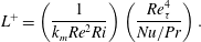
, dimensionless quantities which are determined by the wall fluxes of heat and momentum. As shown by DCT, critical to the transition from intermittent behaviour to fully turbulent behaviour is the parameter
 $L^{+}$
, which can be rewritten in terms of the bulk input external parameters
 $(Re,Ri,Pr)$
and the output parameters
 $(Re_{\unicode[STIX]{x1D70F}},Nu)$
as
 $$\begin{eqnarray}L^{+}=\left(\frac{1}{k_{m}Re^{2}Ri}\right)\left(\frac{Re_{\unicode[STIX]{x1D70F}}^{4}}{Nu/Pr}\right).\end{eqnarray}$$
Consider the scenario where
 $(Re,Ri)$
are fixed and
 $Pr$
is adjusted by varying
 $\unicode[STIX]{x1D705}$
. The first bracket on the right-hand side of (4.2) is thus fixed, and the second bracket includes all parameters that are
 $Pr$
-dependent. The term
 $Re_{\unicode[STIX]{x1D70F}}^{4}$
is a measure of momentum flux (shear stress), and the term
 $Nu/Pr=q_{w}h/(T_{w}\unicode[STIX]{x1D708})$
quantifies the stabilizing effect of stratification. By inspecting the values of
 $Re_{\unicode[STIX]{x1D70F}}$
and
 $Nu$
in table 1 as they vary with
 $Pr$
, (in particular, simulations 3, 6 and 9 which share the same
 $(Re,Ri)$
) it appears that
 $Re_{\unicode[STIX]{x1D70F}}$
increases and
 $Nu/Pr$
decreases as
 $Pr$
increases. In combination, these two effects result in larger values of
 $L^{+}$
. Therefore, at given
 $(Re,Ri)$
values, larger
 $Pr$
enhances the destabilizing wall shear stress and inhibits the stabilizing heat flux. The flow thus becomes more prone to turbulence due to the increase of
 $Pr$
.
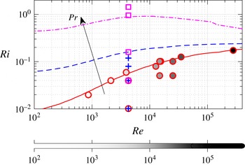
Effect of
 $Pr$
on the intermittency boundary on the
 $(Re,Ri)$
plane. Contours corresponding to
 $L^{+}=200$
, the minimum
 $L^{+}$
value for fully developed turbulence (no intermittency) as proposed by DCT, are constructed using the mixing length model described in § 3. The areas corresponding to
 $L^{+}>200$
are below the various contour lines, plotted with a solid line for
 $Pr=0.7$
, with a dashed line for
 $Pr=7$
and with a dot-dashed line for
 $Pr=70$
. The
 $(Re,Ri)$
combinations for the simulations (see table 1) considered in the present study are marked with circles for
 $Pr=0.7$
, with pluses for
 $Pr=7$
and with squares for
 $Pr=70$
. Varying Reynolds numbers are used in the simulations at
 $Pr=0.7$
, and the fill colour in the circles is made darker for larger values of
 $Re$
to match figure 4.

Figure 6 demonstrates the effect of
 $Pr$
on the intermittency boundary dividing the fully turbulent flow regime from the intermittent regime. Contours corresponding to
 $L^{+}=200$
, i.e. the intermittency boundary proposed by DCT, are plotted on the
 $(Re,Ri)$
plane. At a given
 $Re$
, increasing
 $Pr$
effectively allows fully turbulent flows to exist at higher values of
 $Ri$
. This can be understood from two perspectives. First, as discussed previously, increasing
 $Pr$
destabilizes the flow due to the combined effects of larger shear and smaller stratification. Second,
 $Pr$
reshapes the mean temperature and velocity profiles which results in smaller gradient Richardson number
 $Ri_{g}$
values in the channel gap interior as
 $Pr$
increases (as shown in figure 5) allowing shear to dominate stratification away from the walls. While large values of
 $Pr$
can raise the transitional
 $Ri$
value for a given
 $Re$
, figure 6 suggests that fully developed turbulence is not likely to exist for
 $Ri\gg 1$
, at least within the range of
 $Re$
and
 $Pr$
values which has been investigated, both for the simulations conducted specifically for this paper at
 $Re=4250$
, and the simulations at a range of
 $Re$
presented by DCT, as listed in table 1.
5 Monin–Obukhov similarity scaling
It has been shown in § 4 that
 $Pr$
plays a significant role in the near-wall region by modulating the wall heat flux
 $q_{w}$
, the momentum flux
 $u_{\unicode[STIX]{x1D70F}}^{2}$
and thus the dimensionless parameters such as
 $L^{+}$
and
 $Re_{\unicode[STIX]{x1D70F}}$
. In this section, we turn our attention to our second main theme, i.e. assessing the validity of Monin–Obukhov similarity scaling. We focus on the turbulence in the interior of the channel gap and examine how the turbulence characteristics relate to the wall fluxes
 $q_{w}$
and
 $u_{\unicode[STIX]{x1D70F}}^{2}$
. Scalings for various flow diagnostics are formulated in the context of Monin–Obukhov theory (see details in appendices A and B, and the similar formulations considered independently by Scotti & White (Reference Scotti and White2016)). These predictions are then compared to DNS data shown in figure 7 and the dynamical implications of these scalings are discussed in detail in this section. Simulations specifically performed for the present study, i.e. simulations 1–12 as listed in table 1, which cover a wide range of
 $Pr$
, as well as those performed by DCT, i.e. simulations 13–23, which cover a wide range of
 $Re$
, are included in our discussions.
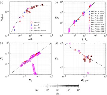
DNS verification of the Monin–Obukhov scalings (5.1), (5.3), (5.4) and (5.7). (a) Equilibrium gradient Richardson number
 $Ri_{g}|_{y=0}$
at midgap, as a function of length scale ratio
 $h/L$
. (b) Buoyancy Reynolds number
 $Re_{b}$
as a function of length scale ratio
 $L^{+}$
.
 $Re_{b}$
values are computed pointwise in
 $y$
for the channel gap interior with
 $y^{+}>50$
. (c) Flux Richardson number
 $Ri_{f}\equiv -B/P$
as a function of gradient Richardson number
 $Ri_{g}$
.
 $Ri_{f}$
and
 $Ri_{g}$
values are computed pointwise in
 $y$
in the channel gap interior with
 $y^{+}>50$
. Symbol types are the same as (b). (d) Turbulent Froude number
 $Fr_{h}$
as a function of midgap gradient Richardson number
 $Ri_{g}$
.
 $Fr_{h}$
is estimated as
 $\unicode[STIX]{x1D700}/(Nu_{\unicode[STIX]{x1D70F}}^{2})$
, where
 $\unicode[STIX]{x1D700}$
and
 $N$
are sampled at midgap
 $y=0$
. Symbol types are the same as in (a). The dashed line corresponds to
 $Fr_{h}=0.95Ri_{g}^{-1/2}$
, the least-squares fit to the scaling (5.7). In (a,d), the fill colours of the circles (corresponding to simulations with
 $Pr=0.7$
) are made darker for larger values of
 $Re$
.

5.1 Equilibrium Richardson number
We first revisit the midgap gradient Richardson number
 $Ri_{g}|_{y=0}$
for fully developed stationary (equilibrium) stratified plane Couette flows as prescribed by Monin–Obukhov scaling. The concept of just such a characteristic equilibrium
 $Ri_{g}$
value was discussed by Turner (Reference Turner1973) in the context of constant flux layers. There also exists a large body of literature considering the ‘stationary Richardson number’ in homogeneous sheared stratified turbulence, e.g. see Shih et al. (Reference Shih, Koseff, Ferziger and Rehmann2000), where the particular value of the gradient Richardson number is imposed by construction, and the references therein. A more recent discussion by Galperin, Sukoriansky & Anderson (Reference Galperin, Sukoriansky and Anderson2007) questioned whether such a unique ‘critical Richardson number’ exists, although the flows considered there differed in several significant ways from the flows considered here. Specifically, and most importantly, stratified plane Couette flow exhibits intermittency for the bulk Richardson number
 $Ri\lesssim O(1)$
. Also, as we discuss in more detail below, the turbulent Prandtl number, i.e. the ratio of eddy diffusivities of heat and momentum, behaves in a qualitatively different manner in stratified plane Couette flow from the behaviour of the ‘quasi-normal scale elimination’ (QNSE) model used in Galperin et al. (Reference Galperin, Sukoriansky and Anderson2007). Under the plausible assumption that a critical Richardson number exists at least in the flow geometry under consideration here, it may help us to assess if the turbulence would be self-sustained if the externally imposed Richardson number matches the equilibrium condition, or if the flow would self-adjust under non-equilibrium conditions (Turner Reference Turner1973). Examples of the adjustment in the latter scenario include the formation of ‘layer’ and ‘interface’ structures through the rearrangement of velocity and density profiles so that the equilibrium Richardson number is maintained everywhere in the vertical direction (see § 10, Turner Reference Turner1973).
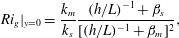
Figure 7(a) compares the midgap equilibrium
 $Ri_{g}|_{y=0}$
values from DNS data (from both the present study and those by DCT crucially at a range of
 $Re$
) with the model prediction (B 3) derived in appendix B, i.e.
 $$\begin{eqnarray}Ri_{g}|_{y=0}=\frac{k_{m}}{k_{s}}\frac{(h/L)^{-1}+\unicode[STIX]{x1D6FD}_{s}}{[(h/L)^{-1}+\unicode[STIX]{x1D6FD}_{m}]^{2}},\end{eqnarray}$$
which suggests that such an equilibrium
 $Ri_{g}$
value is determined solely by the length scale ratio
 $h/L$
(note that
 $k_{m}$
,
 $k_{s}$
,
 $\unicode[STIX]{x1D6FD}_{s}$
and
 $\unicode[STIX]{x1D6FD}_{m}$
are model constants defined in § 3). The data points indeed collapse in figure 7(a) for the wide range of external parameters (in particular, Prandtl number
 $Pr$
, but also Reynolds number
 $Re$
) examined, and the DNS results compare well with the Monin–Obukhov prediction (5.1).
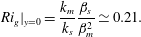
Two scenarios in stratified plane Couette flows arise from (5.1) when
 $h/L$
approaches different limits. First, when
 $h/L\rightarrow \infty$
, the midgap equilibrium
 $Ri_{g}$
saturates at
 $$\begin{eqnarray}Ri_{g}|_{y=0}=\frac{k_{m}}{k_{s}}\frac{\unicode[STIX]{x1D6FD}_{s}}{\unicode[STIX]{x1D6FD}_{m}^{2}}\simeq 0.21.\end{eqnarray}$$
This scenario is at least superficially similar to the discussion of constant-flux layers in ‘very stable’ stratification (Ellison Reference Ellison1957; Turner Reference Turner1973), although as discussed further below, the behaviour of the turbulent Prandtl number is qualitatively different from that assumed by Ellison (Reference Ellison1957). When
 $\unicode[STIX]{x1D709}=h/L\gg 1$
, the linear dependence of Monin–Obukhov functions
 $\unicode[STIX]{x1D6F7}_{m}$
and
 $\unicode[STIX]{x1D6F7}_{s}$
on
 $\unicode[STIX]{x1D709}$
dominates (see (3.11) and (3.12)). Fluid in the channel gap interior does not ‘feel’ the impact of the wall directly (but still indirectly though the wall fluxes
 $u_{\unicode[STIX]{x1D70F}}^{2}$
and
 $q_{w}$
), because the vertical motions are strongly damped by stratification. In the channel gap interior, the distance to the wall
 $y_{w}$
(or the channel gap half-height
 $h$
) becomes irrelevant, as shear and temperature gradients both become constant (by taking the limit of (3.12) at
 $\unicode[STIX]{x1D709}\rightarrow \infty$
), which renders the turbulence close to homogeneous in the wall-normal direction. Interestingly, the maximum stationary
 $Ri_{g}$
reported in homogeneous sheared turbulence is also approximately 0.2 (see e.g. Shih et al.
Reference Shih, Koseff, Ferziger and Rehmann2000). This reinforces the notion that Monin–Obukhov scaling may also apply to such homogeneous triply periodic flows (Chung & Matheou Reference Chung and Matheou2012). There remains some debate as to whether the standard Monin–Obukhov theory holds in the
 $\unicode[STIX]{x1D709}\rightarrow \infty$
limit in a stable atmospheric boundary layer, see for example the discussion on ‘
 $z$
-less’ stratification by Mahrt (Reference Mahrt1999), and any such differences between the standard theory and boundary layer flow are likely linked to the variation of fluxes with height in a real boundary layer. However, the statistically stationary stratified plane Couette flows examined here, which are constant-flux layers by construction, appear to be consistent with the standard Monin–Obukhov theory.
As an aside, we note that this maximum observed Richardson number is close to
 $Ri_{g}=1/4$
which arises in the well-known Miles–Howard criterion for linear normal mode stability of inviscid parallel steady stratified shear flows (Howard Reference Howard1961; Miles Reference Miles1961). This closeness is apparently fortuitous, as the arguments leading to the prediction of the value in (5.2) are entirely constructed under the assumption of statistically stationary turbulent flow. Therefore, it is at least possible that observations of
 $Ri_{g}$
close to
 $1/4$
, as, for example, in the equatorial undercurrent (Smyth & Moum Reference Smyth and Moum2013), are due to turbulent balances, not ‘marginal stability’ of the flow, as argued by Thorpe & Liu (Reference Thorpe and Liu2009), although, it is also important to remember, as shown for example by Pham, Sarkar & Winters (Reference Pham, Sarkar and Winters2013), that the dynamics of the Equatorial Undercurrent is inevitably non-stationary, due to diurnal forcing.
Second, when
 $h/L$
is
 $O(1)$
or smaller, the equilibrium
 $Ri_{g}$
at midgap varies strongly with
 $h/L$
, which can be seen from figure 7(a). Under this scenario, the stabilising effects due to stratification are relatively weak. The direct influence of the walls on the interior turbulence becomes significant, and both
 $h$
and
 $L$
become relevant scales for the channel gap interior.
5.2
$L^{+}$
,
$Re_{b}$
and intermittency


The parameter
 $L^{+}$
is a useful diagnostic quantity to predict if stratified plane Couette flows can sustain a fully turbulent state or become intermittent (as discussed by DCT). On the other hand, the buoyancy Reynolds number
 $Re_{b}\equiv \unicode[STIX]{x1D700}/(\unicode[STIX]{x1D708}N^{2})\sim (\ell _{O}/\unicode[STIX]{x1D702})^{4/3}$
, which describes the scale separation between the Ozmidov scale
 $\ell _{O}$
and the Kolmogorov scale
 $\unicode[STIX]{x1D702}$
, is often used to predict whether small scale turbulence can exist given the level of turbulent dissipation and stratification (see e.g. Riley & Lindborg Reference Riley, Lindborg, Davidson, Kaneda and Sreenivasan2012), typically in homogeneous simulations (Brethouwer et al.
Reference Brethouwer, Billant, Lindborg and Chomaz2007).
A natural question to ask is then whether
 $L^{+}$
and
 $Re_{b}$
are related to each other, at least in stratified plane Couette flows. The analysis in appendix B has, through Monin–Obukhov similarity theory, predicted a linear scaling between
 $L^{+}$
and
 $Re_{b}$
as given by (B 5) shown in appendix B, i.e.
 $$\begin{eqnarray}Re_{b}\sim L^{+}k_{m}.\end{eqnarray}$$
In figure 7(b) this scaling is confirmed from DNS data (shown for simulations 1–12), and has already been noted by Scotti & White (Reference Scotti and White2016) in a more limited range of
 $Ri\leqslant 0.1$
,
 $Re\leqslant 55\,000$
and
 $Pr=1$
.
 $Re_{b}$
estimates presented here are based on
 $\unicode[STIX]{x1D700}$
and
 $N$
values that are sampled pointwise in the vertical direction
 $y$
. However, in open flows, there are different possible choices of averaging volumes for
 $\unicode[STIX]{x1D700}$
and
 $N$
(see e.g. Salehipour, Caulfield & Peltier Reference Salehipour, Caulfield and Peltier2016), and caution needs to be exercised when comparing specific numerical values of
 $Re_{b}$
between different flow geometries, or indeed between different analyses. A reanalysis of DCT’s data (simulations 13–23, not shown) suggests the same linear scaling for a wide range of
 $Re$
and
 $Ri$
. This indicates that the
 $L^{+}$
criterion for predicting intermittency, which is specific to wall-bounded flows, is also linked to this more general
 $Re_{b}$
argument. The critical (minimum)
 $Re_{b}$
for fully developed turbulence, as inferred from the
 $L^{+}>200$
criterion reported by DCT and the scaling (5.3), is approximately 80 (as
 $k_{m}\approx 0.4$
) for stratified plane Couette flows. This critical
 $Re_{b}$
of 80 is close to the cutoff value
 $Re_{b}=100$
between the ‘intermediate’ and ‘energetic’ regimes of Shih et al. (Reference Shih, Koseff, Ivey and Ferziger2005) which is discussed in detail in § 6, although one needs to be careful about whether the
 $Re_{b}$
value is a ‘bulk’ or local estimate when comparing the numerical values. Here simulation 12 is in the intermediate regime (
 $Re_{b}<35$
, see figure 7
b), and in what follows, we focus instead on the other simulations (
 $Re_{b}>60$
) which are close to or within this ‘energetic’ regime in terms of the
 $Re_{b}$
value.
5.3 Turbulent Prandtl number
In appendix B, it is shown through scaling arguments that the flux Richardson number
 $Ri_{f}$
is proportional to
 $Ri_{g}$
. The particular scaling derived in appendix B is given by (B 7) i.e.
 $$\begin{eqnarray}Ri_{f}\sim Ri_{g},\end{eqnarray}$$
and is compared to DNS results (simulations 1–12) in figure 7(c). In general,
 $Ri_{f}$
is proportional to
 $Ri_{g}$
with a multiplicative constant of approximately unity, which is consistent with DCT. The group of points which appear to be outliers, correspond to simulation 12 (
 $Pr=70,Ri=1.44$
). As discussed previously, the atypical behaviour associated with this simulation is likely to be due to low-
 $Re_{b}$
, and hence inherently viscously dominated effects.
With the turbulent viscosity
 $\unicode[STIX]{x1D708}_{t}$
defined through the flux gradient relation
 $$\begin{eqnarray}\unicode[STIX]{x1D708}_{t}\equiv -\frac{\langle u^{\prime }v^{\prime }\rangle }{S},\end{eqnarray}$$
and turbulent diffusivity
 $\unicode[STIX]{x1D705}_{t}$
defined in (A 5), the turbulent Prandtl number
 $Pr_{t}\equiv \unicode[STIX]{x1D708}_{t}/\unicode[STIX]{x1D705}_{t}$
can be expressed as
 $$\begin{eqnarray}Pr_{t}=\frac{Ri_{g}}{Ri_{f}}.\end{eqnarray}$$
The
 $Ri_{f}\simeq Ri_{g}$
scaling can thus be interpreted alternatively as the turbulent Prandtl number
 $Pr_{t}$
being approximately unity, which is consistent with the Reynolds analogy, as noted independently by Scotti & White (Reference Scotti and White2016). This result can be derived from Monin–Obukhov theory (appendix B) and is consistent with DNS data for the present study (simulations 1–12) shown in figure 7(c), as well as from revisited DCT datasets (simulations 13–23) which exhibit the same behaviour (not shown).
 $Pr_{t}$
is often parameterized as a function of
 $Ri_{g}$
in the literature (see, for example, Venayagamoorthy & Stretch Reference Venayagamoorthy and Stretch2010).
 $Pr_{t}$
being unity, as we observe in stratified plane Couette flows (see figure 7
c), appears to be typical for gradient Richardson numbers
 $Ri_{g}<0.2$
which are sufficiently small in this context – again, one needs to be careful about the exact definition of
 $Ri_{g}$
when comparing across different studies, and also it is necessary to remember that this is distinct from keeping the bulk Richardson number
 $Ri$
(set by the boundary conditions) small. This observation is consistent with previous studies of stably stratified wall-bounded flow simulations (Armenio & Sarkar Reference Armenio and Sarkar2002; García-Villalba & del Álamo Reference García-Villalba and del Álamo2011; García-Villalba et al.
Reference García-Villalba, Azagra, Uhlmann and Nagel2011a
) and in homogeneous stratified turbulence (Rohr & Van Atta Reference Rohr and Van Atta1987; Chung & Matheou Reference Chung and Matheou2012).
The behaviour of
 $Pr_{t}$
becomes more complex at higher values of
 $Ri_{g}$
, i.e. for
 $Ri_{g}>0.2$
(Taylor, Sarkar & Armenio Reference Taylor, Sarkar and Armenio2005; Venayagamoorthy & Stretch Reference Venayagamoorthy and Stretch2010; Karimpour & Venayagamoorthy Reference Karimpour and Venayagamoorthy2014, Reference Karimpour and Venayagamoorthy2015; Salehipour & Peltier Reference Salehipour and Peltier2015; Wilson & Venayagamoorthy Reference Wilson and Venayagamoorthy2015). However, turbulent flows with larger gradient Richardson numbers
 $Ri_{g}>0.2$
do not appear to be accessible in stratified plane Couette flows, for reasons that have been discussed in § 5.1. There also exist
 $Re_{b}$
-based parameterizations for
 $Pr_{t}$
in the literature. Shih et al. (Reference Shih, Koseff, Ivey and Ferziger2005) and Salehipour & Peltier (Reference Salehipour and Peltier2015) reported
 $Pr_{t}$
approaching order unity for intermediate to large values of
 $Re_{b}$
, which is consistent with our observations. Salehipour & Peltier (Reference Salehipour and Peltier2015) also observed larger than
 $O(1)$
values of
 $Pr_{t}$
when the values of
 $Re_{b}$
are small, i.e.
 $O(1)$
to
 $O(10)$
. This is consistent with our outlier group (simulation 12) in figure 7(c) whose
 $Re_{b}$
value is
 $O(10)$
(see figure 7
b) and the
 $Pr_{t}$
value is larger than unity (
 $Ri_{g}\gg Ri_{f}$
).
Crucially, all the evidence points towards
 $Pr_{t}\sim O(1)$
while the flow is turbulent, with the flow becoming intermittent before
 $Ri_{g}$
reaching large values. This is qualitatively different behaviour to that assumed by Ellison (Reference Ellison1957), who stated that ‘it seems more likely’ that turbulence could be ‘maintained’ at large values of
 $Ri_{g}$
with still finite
 $Ri_{f}<1$
, and so, from (5.6) and consequences derived from it with further turbulence modelling assumptions, Ellison (Reference Ellison1957) was led to the conclusion that
 $Pr_{t}$
inevitably reaches large values. Galperin et al. (Reference Galperin, Sukoriansky and Anderson2007) analogously arrived at the conclusion that
 $Pr_{t}$
reaches large values in strongly stratified, yet still ‘turbulent’ flows, in the relatively weak sense that the eddy diffusivities (particularly in the horizontal) remain elevated above molecular values. A potential major point of difference leading to this apparent qualitative discrepancy in the behaviour of the turbulent Prandtl number is the central role played in open flows of propagating internal waves, which is not possible in stratified plane Couette flow.
5.4 Realizability of strongly stratified regime
Finally, we test the scaling in (B 11) in appendix B, i.e.
 $$\begin{eqnarray}Fr_{h}\sim \frac{1}{\sqrt{Ri_{g}}},\end{eqnarray}$$
for the turbulent Froude number
 $Fr_{h}$
. Figure 7(d) shows the DNS results for which an empirical scaling of
 $$\begin{eqnarray}Fr_{h}\simeq \frac{0.95}{\sqrt{Ri_{g}}}\end{eqnarray}$$
applies, which is consistent with the Monin–Obukhov prediction in appendix B. The outlier once again corresponds to simulation 12 for which the
 $Re_{b}$
value may not be high enough for the inertially dominated forward cascade assumption underlying (B 8), i.e.
 $\unicode[STIX]{x1D700}={U^{\prime }}^{3}/\ell _{h}$
, to hold.
Given that the maximum
 $Ri_{g}$
in fully developed stratified plane Couette flow is approximately 0.2 (see § 5.1), the minimum
 $Fr_{h}$
that can be obtained in the interior of an stratified plane Couette flow (at large enough
 $Re_{b}$
) is approximately 2, following (5.8). However, for the turbulence to reach the strongly stratified regime, it is typically argued that
 $Fr_{h}$
needs to be smaller than 0.02 (Brethouwer et al.
Reference Brethouwer, Billant, Lindborg and Chomaz2007). Therefore, the strongly stratified regime, which is characterized by layering in the density field with characteristic vertical length scale
 $U^{\prime }/N$
, may be fundamentally non-realizable in stratified plane Couette flows, at least under the equilibrium conditions we have been considering. Once again, it is important to emphasize that it is the midgap gradient Richardson number
 $Ri_{g}$
which cannot become large in quasi-steady turbulent stratified plane Couette flow, for any choice of
 $Re$
and
 $Ri$
set by the boundary conditions.
5.5 Summary
To summarize the results in § 5, we have identified certain generic characteristics of the turbulence in the interior regions of stratified plane Couette flows. We find that: the length scale ratio
 $h/L$
determines the midgap
 $Ri_{g}$
;
 $Re_{b}$
scales linearly with
 $L^{+}\equiv L/\unicode[STIX]{x1D6FF}_{\unicode[STIX]{x1D708}}$
;
 $Pr_{t}$
is of order unity for the range of accessible
 $Ri_{g}$
associated with turbulence; and
 $Fr_{h}$
is proportional to
 $Ri_{g}^{-1/2}$
. The scalings, consistent with, and extending the observations of Scotti & White (Reference Scotti and White2016) into the crucially important regime where the externally set bulk
 $Ri>0.1$
, apply not only to the DNS performed for the present study which cover a wide range of
 $Pr$
(simulations 1–12), but also to those by DCT as listed in table 1 which covered a wider range of
 $Re$
(simulations 13–23). These characteristics of stratified plane Couette flows fundamentally relate to the fact that it is the upper and lower walls which impose momentum and heat fluxes on the fluids. These fluxes then dictate the self-similar behaviour of both the mean flow (as characterized by
 $Ri_{g}$
) and the turbulence (as characterized by
 $Re_{b}$
,
 $Pr_{t}$
and
 $Fr_{h}$
) in the interior. These results are expected to hold not only for stratified plane Couette flows but also for other constant-flux layers to which the Monin–Obukhov scaling applies. These Monin–Obukhov scalings are intended for regions sufficiently far from the walls. Through the wide range of Prandtl numbers examined, our DNS data suggest that the dynamics away from the walls is
 $Pr$
-independent for given wall fluxes.
6 Mixing and its parameterization
6.1 Osborn formulation for stratified plane Couette flow
Now we turn our attention to the third main theme of interest, namely the parameterization of mixing. Here we use the framework proposed by Osborn (Reference Osborn1980) to formulate a parameterization for the turbulent diffusivity
 $\unicode[STIX]{x1D705}_{t}\equiv -\langle \unicode[STIX]{x1D70C}^{\prime }v^{\prime }\rangle /(\text{d}\overline{\unicode[STIX]{x1D70C}}/\text{d}y)=-B/N^{2}$
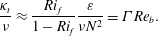
. As described in appendix C, key to this formulation is the turbulent flux coefficient,
 $\unicode[STIX]{x1D6E4}\equiv B/\unicode[STIX]{x1D700}\approx Ri_{f}/(1-Ri_{f})$
. With
 $\unicode[STIX]{x1D6E4}$
appropriately parameterized, the Osborn formulation yields an expression for
 $\unicode[STIX]{x1D705}_{t}$
, i.e.
 $$\begin{eqnarray}\frac{\unicode[STIX]{x1D705}_{t}}{\unicode[STIX]{x1D708}}\approx \frac{Ri_{f}}{1-Ri_{f}}\frac{\unicode[STIX]{x1D700}}{\unicode[STIX]{x1D708}N^{2}}=\unicode[STIX]{x1D6E4}Re_{b}.\end{eqnarray}$$
It is important to appreciate that key aspects of the Osborn (Reference Osborn1980) framework are based on the theoretical considerations of Ellison (Reference Ellison1957) and the experimental data of Britter (Reference Britter1974), both associated with stratified flows in the presence of boundary forcing and thus expected to have at least some similar properties to the turbulence in stratified plane Couette flows. Osborn (Reference Osborn1980), following Ellison (Reference Ellison1957), postulated that
 $\unicode[STIX]{x1D6E4}\leqslant 0.2$
, or equivalently
 $Ri_{f}\leqslant 0.15$
, although the inequality in Osborn’s original paper has often been ignored subsequently. Interestingly, the experimental data by Britter (Reference Britter1974) (see e.g. pp. 8–37 of the thesis) led to his conclusion that ‘a critical Richardson flux number (i.e.
 $Ri_{f}$
) of approximately 0.2 is predicted’. This is entirely consistent with our results presented in § 5 that
 $$\begin{eqnarray}Ri_{f}\simeq Ri_{g}\lesssim 0.2\end{eqnarray}$$
in stratified plane Couette flows for turbulence to be maintained, although as already noted we observe the turbulent Prandtl number remaining of order one, unlike in the model developed by Ellison (Reference Ellison1957). Indeed, using this scaling,
 $\unicode[STIX]{x1D6E4}$
can be written as a function of the gradient Richardson number
 $Ri_{g}$
:
 $$\begin{eqnarray}\unicode[STIX]{x1D6E4}\approx \frac{Ri_{g}}{1-Ri_{g}},\end{eqnarray}$$
remembering that
 $Ri_{g}$
appears to have an upper bound above which turbulence cannot be maintained, even for asymptotically large
 $Re$
(see figure 18 of DCT), In the literature, however,
 $\unicode[STIX]{x1D6E4}$
is often parameterized as a function of
 $Re_{b}$
(see e.g. Shih et al.
Reference Shih, Koseff, Ivey and Ferziger2005). The connection between the
 $Ri_{g}$
-based and
 $Re_{b}$
-based scalings for
 $\unicode[STIX]{x1D6E4}$
is discussed further in § 6.3.1. It follows from (6.1) and (6.3) that
 $$\begin{eqnarray}\frac{\unicode[STIX]{x1D705}_{t}}{\unicode[STIX]{x1D708}}\approx \frac{Ri_{g}}{1-Ri_{g}}Re_{b}\end{eqnarray}$$
in the context of stratified plane Couette flows. Noting that
 $Pr_{t}\equiv \unicode[STIX]{x1D708}_{t}/\unicode[STIX]{x1D705}_{t}\approx 1$
in stratified plane Couette flows (as shown in § 5) and as also noted by Scotti & White (Reference Scotti and White2016), we can also approximate the turbulent viscosity
 $\unicode[STIX]{x1D708}_{t}$
with the same scaling for
 $\unicode[STIX]{x1D705}_{t}$
in (6.4), i.e.
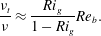 $$\begin{eqnarray}\frac{\unicode[STIX]{x1D708}_{t}}{\unicode[STIX]{x1D708}}\approx \frac{Ri_{g}}{1-Ri_{g}}Re_{b}.\end{eqnarray}$$
 $\unicode[STIX]{x1D705}_{t}$
and
 $\unicode[STIX]{x1D708}_{t}$
, as defined by (A 5) and (5.5), and both normalized by
 $\unicode[STIX]{x1D708}$
, as a function of
 $Re_{b}$
;
 $\unicode[STIX]{x1D705}_{t}$
,
 $\unicode[STIX]{x1D708}_{t}$
and
 $Re_{b}$
values are computed pointwise in
 $y$
in the channel gap interior with
 $y^{+}>50$
. Scaling laws of
 $\unicode[STIX]{x1D705}_{t}/\unicode[STIX]{x1D708}=0.2Re_{b}$
(Osborn Reference Osborn1980) plotted with a solid line, and
 $\unicode[STIX]{x1D705}_{t}/\unicode[STIX]{x1D708}=2Re_{b}^{1/2}$
(Shih et al.
Reference Shih, Koseff, Ivey and Ferziger2005) plotted with a dashed line, are also shown.

6.2 Numerical results
These
 $\unicode[STIX]{x1D705}_{t}$
and
 $\unicode[STIX]{x1D708}_{t}$
values are estimated directly using their definitions through the flux gradient relation (A 5) and (5.5) at all locations in the wall-normal direction
 $y$
that are at least 50 wall units (
 $y^{+}>50$
) away from the walls, where the local equilibrium (A 3) is expected to hold (García-Villalba et al.
Reference García-Villalba, Azagra and Uhlmann2011b
). These results are first plotted in figure 8 to test the
 $Re_{b}$
-based parameterizations that are commonly seen in the literature, e.g. those reviewed by Ivey et al. (Reference Ivey, Winters and Koseff2008) and also discussed in Scotti & White (Reference Scotti and White2016). Our results are plotted in figure 9 to validate the scalings (6.4) and (6.5). Simulation 12, in which the flow is viscously controlled and exhibits spuriously small (
 $O(1)$
or smaller) or negative (counter-gradient) values of
 $\unicode[STIX]{x1D705}_{t}/\unicode[STIX]{x1D708}$
or
 $\unicode[STIX]{x1D708}_{t}/\unicode[STIX]{x1D708}$
, is not included in the plots to allow the discussion to stay focused on the fully turbulent simulations.
Figure 8 compares the DNS results of
 $\unicode[STIX]{x1D705}_{t}/\unicode[STIX]{x1D708}$
against the classical
 $Re_{b}$
-based parameterizations of Osborn (Reference Osborn1980) and Shih et al. (Reference Shih, Koseff, Ivey and Ferziger2005). The DNS data points in figure 8 are sampled locally (pointwise) at various
 $y$
locations across the channel gap interior of stratified plane Couette flows. Within each simulation, the
 $Re_{b}$
value stays relatively constant, while the diffusivities span a wider range – the latter is somewhat expected because
 $\unicode[STIX]{x1D705}_{t}$
and
 $\unicode[STIX]{x1D708}_{t}$
scale linearly with the mixing lengths
 $\ell _{s}^{\ast }$
and
 $\ell _{m}^{\ast }$
respectively, both of which increase with the wall distance
 $y_{w}$
, as described in § 3.1. These
 $Re_{b}$
-based scalings are effective in describing the homogeneous flow dataset of Shih et al. (Reference Shih, Koseff, Ivey and Ferziger2005), but they do not provide a good agreement with our DNS data from stratified plane Couette flows which are inherently inhomogeneous due in particular to the presence of the wall. The data for
 $\unicode[STIX]{x1D708}_{t}$
, which are also plotted in figure 8, behave similarly to
 $\unicode[STIX]{x1D705}_{t}$
, since the turbulent Prandtl number
 $Pr_{t}\equiv \unicode[STIX]{x1D708}_{t}/\unicode[STIX]{x1D705}_{t}$
is approximately unity (as shown in § 5.3).
Figure 9 compares the DNS data against the scalings (6.4) and (6.5). The collapse of the DNS data improves significantly when
 $Ri_{g}$
is included in the parameterizations, as they capture the critical (linear) dependence of
 $Ri_{f}$
on
 $Ri_{g}$
. At sufficiently large values of
 $Re_{b}$
, i.e.
 $Re_{b}\gtrsim 60$
, the
 $\unicode[STIX]{x1D705}_{t}/\unicode[STIX]{x1D708}\sim \unicode[STIX]{x1D708}_{t}/\unicode[STIX]{x1D708}\sim Re_{b}Ri_{g}/(1-Ri_{g})$
scaling, based on the turbulent kinetic energy budget argument by Osborn (Reference Osborn1980) and incorporating Monin–Obukhov scaling for constant-flux layers to account for the importance of the (coupled) value of
 $Ri_{g}$
, provides an accurate description of the turbulent diffusivity in stratified plane Couette flows. It is certainly of interest that the Osborn scaling appears to hold, at least qualitatively, even though the underlying assumption of Ellison (Reference Ellison1957) (on which the Osborn scaling is at least partially based) that
 $Pr_{t}$
becomes large is violated in stratified plane Couette flow. We further discuss this scaling with respect to other previously proposed scalings in the next subsection.
 $\unicode[STIX]{x1D705}_{t}$
and
 $\unicode[STIX]{x1D708}_{t}$
, both normalized by
 $\unicode[STIX]{x1D708}$
, as a function of
 $Re_{b}Ri_{g}/(1-Ri_{g})$
;
 $\unicode[STIX]{x1D705}_{t}$
,
 $\unicode[STIX]{x1D708}_{t}$
,
 $Re_{b}$
and
 $Ri_{g}$
values are computed pointwise in
 $y$
in the channel gap interior with
 $y^{+}>50$
. The dashed line marks equality between the abscissa and the ordinate.

6.3 Discussion
6.3.1
$\unicode[STIX]{x1D6E4}$
versus
$Re_{b}$


The Shih et al. (Reference Shih, Koseff, Ivey and Ferziger2005) scalings parameterize the turbulent flux coefficient
 $\unicode[STIX]{x1D6E4}$
as a function of the buoyancy Reynolds number
 $Re_{b}$
, whereas in the context of stratified plane Couette flow, we propose to parameterize
 $\unicode[STIX]{x1D6E4}$
as a function of the gradient Richardson number
 $Ri_{g}$
, i.e.
 $\unicode[STIX]{x1D6E4}\approx Ri_{g}/(1-Ri_{g})$
. Here we discuss our results further with respect to the two approaches. Following Shih et al. (Reference Shih, Koseff, Ivey and Ferziger2005), for
 $7<Re_{b}<100$
, i.e. the ‘intermediate’ regime, a constant turbulent flux coefficient of
 $\unicode[STIX]{x1D6E4}=0.2$
, as originally proposed by Osborn (Reference Osborn1980) as an upper bound, is used. For
 $Re_{b}>100$
, i.e. the ‘energetic’ regime,
 $\unicode[STIX]{x1D6E4}$
was observed by Shih et al. (Reference Shih, Koseff, Ivey and Ferziger2005) to decrease with
 $Re_{b}$
as
 $\unicode[STIX]{x1D6E4}\propto Re_{b}^{-1/2}$
, although their data only extend to
 $Re_{b}\simeq 900$
. The scaling for
 $Re_{b}>100$
appears to be consistent with numerical data of mixing layers (Salehipour & Peltier Reference Salehipour and Peltier2015) and field observations (Davis & Monismith Reference Davis and Monismith2011; Walter et al.
Reference Walter, Squibb, Woodson, Koseff and Monismith2014). One shortcoming of this scaling is, however, that the value of
 $\unicode[STIX]{x1D705}_{t}/\unicode[STIX]{x1D708}=\unicode[STIX]{x1D6E4}Re_{b}\propto Re_{b}^{1/2}$
becomes infinite when one considers the mixing of a passive scalar, since
 $Re_{b}\rightarrow \infty$
as
 $N^{2}\rightarrow 0$
and
 $\unicode[STIX]{x1D700}$
and
 $\unicode[STIX]{x1D708}$
remain finite. In contrast, experiments by Holford & Linden (Reference Holford and Linden1999) suggested that the eddy diffusivity approaches a finite value in the zero stratification limit. Moreover, Chung & Matheou (Reference Chung and Matheou2012) also reported saturation of eddy diffusivity for large-to-infinite values of
 $Re_{b}$
and offered a phenomenological explanation from the perspective of competing length scales.
Turbulent flux coefficient
 $\unicode[STIX]{x1D6E4}$
(as defined in (C 3)) approximated by
 $Ri_{g}/(1-Ri_{g})$
, where
 $Ri_{g}$
is evaluated at midgap, plotted as a function of
 $Re_{b}$
which is approximated by
 $k_{m}L^{+}$
(as shown in figure 7
b). Symbols correspond to DNS data. Lines correspond to two different Monin-Obukhov predictions: at
 $Re=4250$
(the same
 $Re$
value as the shown DNS results) plotted with a solid line; and at
 $Re=42\,500$
plotted as a dashed line. Power-law scalings
 $\unicode[STIX]{x1D6E4}\propto Re_{b}^{n}$
with various
 $n$
values are plotted with dot-dashed lines marked with the values of
 $n$
.

The scalings (6.4) and (6.5), by including the
 $Ri_{g}$
-dependence, circumvent this problem at the zero stratification limit where
 $Re_{b}\rightarrow \infty$
as
 $Ri\rightarrow 0$
, as
 $\unicode[STIX]{x1D6E4}\propto Re_{b}^{-1}$
in the limit of
 $Re_{b}\rightarrow \infty$
(as shown in figure 10). These scalings also provide a convenient framework to interpret the change of power-law exponent in
 $Re_{b}$
in the scaling of
 $\unicode[STIX]{x1D6E4}$
(Barry et al.
Reference Barry, Ivey, Winters and Imberger2001; Shih et al.
Reference Shih, Koseff, Ivey and Ferziger2005). This is demonstrated in figure 10, where the characteristic values of turbulent flux coefficient
 $\unicode[STIX]{x1D6E4}$
in the interior of stratified plane Couette flow, as approximated by
 $Ri_{g}/(1-Ri_{g})$
, are plotted against the corresponding
 $Re_{b}$
values. The Monin–Obukhov predictions from the model presented in § 3 are also shown in figure 10 for two values of bulk Reynolds number
 $Re$
, i.e.
 $Re=4250$
and
 $Re=42\,500$
.
As shown in figure 10, when
 $Re_{b}$
is smaller than
 $O(100)$
, which corresponds to the
 $h/L>1$
regime in terms of the characteristic
 $Ri_{g}$
value (see figure 7
a),
 $Ri_{g}$
remains a constant value of approximately
 $0.2$
at midgap as given in (5.2). The characteristic turbulent flux coefficient
 $\unicode[STIX]{x1D6E4}\approx Ri_{g}/(1-Ri_{g})\approx 0.25$
is thus a constant. This regime is reminiscent of the Shih et al. (Reference Shih, Koseff, Ivey and Ferziger2005) ‘intermediate’ regime where
 $\unicode[STIX]{x1D6E4}$
is a constant of 0.2 independent of
 $Re_{b}$
, the upper bound as argued by Osborn (Reference Osborn1980). Consequently,
 $\unicode[STIX]{x1D705}_{t}/\unicode[STIX]{x1D708}=\unicode[STIX]{x1D6E4}Re_{b}\propto Re_{b}$
in this regime. This regime may be thought of as a saturated regime for
 $\unicode[STIX]{x1D6E4}$
, as
 $Ri_{g}$
is close to its maximum value for sustained turbulence, consistent with the underlying assumptions of Osborn (Reference Osborn1980).
When
 $Re_{b}$
is large, e.g.
 $Re_{b}>O(1000)$
for
 $Re=4250$
, which corresponds to the
 $h/L\ll 1$
limit in terms of
 $Ri_{g}$
(figure 7
a), the characteristic
 $Ri_{g}$
can be estimated via (B 3) by taking the limit of
 $h/L\rightarrow 0$
or
 $L^{+}\rightarrow \infty$
, which yields
 $$\begin{eqnarray}Ri_{g}=\frac{k_{m}}{k_{s}}\frac{h}{L}=\frac{k_{m}}{k_{s}}\frac{Re_{\unicode[STIX]{x1D70F},\infty }}{L^{+}}\approx \frac{k_{m}^{2}}{k_{s}}\frac{Re_{\unicode[STIX]{x1D70F},\infty }}{Re_{b}},\end{eqnarray}$$
where
 $Re_{\unicode[STIX]{x1D70F},\infty }$
denotes the friction Reynolds number for the case of passive scalar (
 $L^{+}\rightarrow \infty ,Re_{b}\rightarrow \infty$
). With
 $Ri_{g}\ll 1$
in this limit,
 $\unicode[STIX]{x1D6E4}\approx Ri_{g}/(1-Ri_{g})\approx Ri_{g}$
. Following (6.6), the turbulent flux coefficient
 $\unicode[STIX]{x1D6E4}\approx Ri_{g}\propto Re_{b}^{-1}$
holds for large
 $Re_{b}$
in the limit of zero Richardson number. It is important to appreciate that this is not in itself inconsistent with the Osborn (Reference Osborn1980) argument, as 0.2 is the upper bound he proposes for
 $\unicode[STIX]{x1D6E4}$
. It follows from (6.6) that, in the limit of
 $Re_{b}\rightarrow \infty$
,
 $\unicode[STIX]{x1D705}_{t}/\unicode[STIX]{x1D708}=\unicode[STIX]{x1D6E4}Re_{b}=k_{m}^{2}k_{s}^{-1}Re_{\unicode[STIX]{x1D70F},\infty }$
approaches a constant which depends solely on
 $Re_{\unicode[STIX]{x1D70F},\infty }$
(which itself is a function of the bulk Reynolds number
 $Re$
). This regime corresponds to the scenario of mixing a nearly passive scalar, a regime that finds no counterpart in the regimes presented in Shih et al. (Reference Shih, Koseff, Ivey and Ferziger2005). As is apparent in figure 10, this regime only really becomes clearly identifiable for
 $Re_{b}\gtrsim 1000$
, larger values than those presented in Shih et al. (Reference Shih, Koseff, Ivey and Ferziger2005).
There exists a transitional regime where
 $\unicode[STIX]{x1D6E4}$
decays monotonically with
 $Re_{b}$
, but with a slower rate than the
 $\unicode[STIX]{x1D6E4}\propto Re_{b}^{-1}$
power law in the weakly stratified limit. This transitional regime at least superficially resembles the Shih et al. (Reference Shih, Koseff, Ivey and Ferziger2005) ‘energetic’ regime where
 $\unicode[STIX]{x1D6E4}\propto Re_{b}^{-1/2}$
and
 $\unicode[STIX]{x1D705}_{t}/\unicode[STIX]{x1D708}\propto Re_{b}^{1/2}$
in the sense that
 $\unicode[STIX]{x1D6E4}$
starts to decrease with
 $Re_{b}$
. Of course it is important to remember that this resemblance may be entirely fortuitous, due not least to the necessity of connecting two different asymptotic regimes, and the marked difference of the two flow geometries and forcing mechanisms of the turbulence. The critical
 $Re_{b}$
, which marks the transition from the small-
 $Re_{b}$
regime to this intermediate-
 $Re_{b}$
regime, appears to be approximately 100 for
 $Re=4250$
. However, as shown by Monin–Obukhov predictions plotted in figure 10 for
 $Re=42\,500$
, the exact value of the critical
 $Re_{b}$
is not unique but rather moves to larger values for larger
 $Re$
, and also the specific numerical values are dependent on the averaging volumes for
 $\unicode[STIX]{x1D700}$
and
 $N$
in spatially inhomogeneous flows.
To summarize, in the small-
 $Re_{b}$
regime with
 $Re_{b}\lesssim 100$
,
 $\unicode[STIX]{x1D6E4}$
and
 $Ri_{g}$
are independent of
 $Re_{b}$
, and in the weakly stratified
 $Re_{b}\gtrsim 1000$
regime with small
 $Ri$
,
 $\unicode[STIX]{x1D6E4}\approx Ri_{g}\propto Re_{b}^{-1}$
where the mixing resembles that of a nearly passive scalar. It is within the transitional regime between these two where
 $Ri_{g}$
, and thus also
 $\unicode[STIX]{x1D6E4}\approx Ri_{g}/(1-Ri_{g})$
, both become dependent on
 $Re_{b}$
. The coupling between
 $Ri_{g}$
and
 $Re_{b}$
, as is dictated by Monin–Obukhov scalings in stratified plane Couette flow, may offer some explanation for the commonly observed variations of
 $\unicode[STIX]{x1D6E4}$
with respect to
 $Re_{b}$
(as presented, for example, in Shih et al. (Reference Shih, Koseff, Ivey and Ferziger2005)). It is very important to stress that this picture emerges from wall-bounded stratified shear flows, consistent with the arguments and data underpinning the model of Osborn (Reference Osborn1980). In particular, the picture depends strongly on the observation in stratified plane Couette flow that
 $Ri_{f}\simeq Ri_{g}$
and that
 $Ri_{g}\lesssim 0.2$
for sustained turbulence.
6.3.2
$\unicode[STIX]{x1D6E4}$
versus
$Fr_{h}$


A recent study by Maffioli et al. (Reference Maffioli, Brethouwer and Lindborg2016) utilized the parameter
 $Fr_{h}$
to scale turbulent flux coefficient
 $\unicode[STIX]{x1D6E4}$
in triply periodic body-forced turbulence. Critically its forcing is very different from the forcing which we consider. In stratified plane Couette flow, the forcing at the boundary has to penetrate into the interior to drive turbulent mixing, while the forcing in the flow considered by Maffioli et al. (Reference Maffioli, Brethouwer and Lindborg2016) is introduced throughout the interior of the flow, and so there is no dynamical ‘barrier’ to the energy being available to stratified turbulent mixing throughout the flow. For the
 $Fr_{h}>1$
regime, which corresponds to our small-
 $Ri_{g}$
weakly stratified regime, they proposed that
 $\unicode[STIX]{x1D6E4}\propto Fr_{h}^{-2}$
. A similar dependence of
 $\unicode[STIX]{x1D6E4}$
on the bulk Froude number
 $Fr_{0}=U/\sqrt{G^{\prime }H\cos \unicode[STIX]{x1D703}}$
(defined using characteristic scales for the current velocity
 $U$
along a slope of angle
 $\unicode[STIX]{x1D703}$
to the horizontal, depth
 $H$
and reduced gravity
 $G^{\prime }\cos \unicode[STIX]{x1D703}$
) i.e.
 $\unicode[STIX]{x1D6E4}\propto Fr_{0}^{-2}$
, has also been reported for relatively weakly stratified density currents when
 $Fr_{0}\gg 1$
(Wells, Cenedese & Caulfield Reference Wells, Cenedese and Caulfield2010). It has been shown that
 $Fr_{h}\propto Ri_{g}^{-1/2}$
holds in stratified plane Couette flows (see § 5.4), and therefore the
 $\unicode[STIX]{x1D6E4}\propto Fr_{h}^{-2}$
scaling for
 $\unicode[STIX]{x1D6E4}$
is consistent with our approximation
 $\unicode[STIX]{x1D6E4}\approx Ri_{g}/(1-Ri_{g})\approx Ri_{g}$
(for small
 $Ri_{g}$
). For the small-
 $Fr_{h}$
regime, Maffioli et al. (Reference Maffioli, Brethouwer and Lindborg2016) reported a
 $\unicode[STIX]{x1D6E4}$
value approaching a constant 0.33 at
 $Fr_{h}$
values of
 $O(10^{-2})$
which are accessible in their forced simulations. In stratified plane Couette flows, where the minimum
 $Fr_{h}$
is of
 $O(1)$
as shown in figure 7(d), our results suggest a fixed value of
 $0.2/(1-0.2)=0.25$
that is closer to the upper bound of the Osborn (Reference Osborn1980) formulation, i.e.
 $\unicode[STIX]{x1D6E4}=0.2$
, which is also the value reported by Wells et al. (Reference Wells, Cenedese and Caulfield2010) in their intermediate
 $Fr_{0}\sim 1$
regime.
6.3.3 Non-monotonic mixing?
Pioneering work on turbulent mixing in stratified flows (Linden Reference Linden1979, Reference Linden1980; Fernando Reference Fernando1991; Park, Whitehead & Gnanadeskian Reference Park, Whitehead and Gnanadeskian1994; Holford & Linden Reference Holford and Linden1999) revealed the possibility of non-monotonic behaviour in the stratified mixing, i.e. the buoyancy flux does not necessarily increase monotonically but rather can plateau and then decrease with increasing stratification. Non-monotonic mixing was proposed to be the mechanism for the formation of generic features in stratified fluids such as relatively well mixed and deep ‘layers’ separated by relatively shallow and sharp ‘interfaces’, as originally proposed by Phillips (Reference Phillips1972). Such non-monotonic mixing has also been observed in time-dependent stratified shear layers (Caulfield & Peltier Reference Caulfield and Peltier2000; Smyth, Moum & Caldwell Reference Smyth, Moum and Caldwell2001; Mashayek, Caulfield & Peltier Reference Mashayek, Caulfield and Peltier2013; Salehipour & Peltier Reference Salehipour and Peltier2015). Potentially associated spontaneous layer formation has been observed in stratified Taylor–Couette flows in the annular region between two concentric cylinders (Oglethorpe, Caulfield & Woods Reference Oglethorpe, Caulfield and Woods2013) and in flows where the mixing is induced by translating rods (Park et al. Reference Park, Whitehead and Gnanadeskian1994; Holford & Linden Reference Holford and Linden1999).
In fully developed turbulent stratified plane Couette flow, however, such non-monotonic mixing is not observed. The turbulent flux coefficient
 $\unicode[STIX]{x1D6E4}\equiv B/\unicode[STIX]{x1D700}$
, which measures the buoyancy flux in dimensionless form, increases monotonically with
 $Ri_{g}$
, a dimensionless measure of the stratification. We hypothesize that this behaviour is due to the range of
 $Ri_{g}$
which is accessible in turbulent stratified plane Couette flows where the maximum gradient Richardson number is approximately 0.2 (as discussed in § 5.1). Effectively, it appears that stratified plane Couette flows can only access the weakly stratified ‘left flank’ of the non-monotonic mixing curve with stratification postulated by Phillips (Reference Phillips1972) and observed widely in experiments (see, for example, the classic review of Linden (Reference Linden1979)).
6.3.4 Effect of Prandtl number
Throughout our discussion in this section, there is no explicit dependence of the normalized values of
 $\unicode[STIX]{x1D705}_{t}/\unicode[STIX]{x1D708}$
(or
 $\unicode[STIX]{x1D708}_{t}/\unicode[STIX]{x1D708}$
) on the molecular Prandtl number
 $Pr$
. This is probably due to the fact that the
 $Re_{b}$
values examined here are sufficiently large, i.e.
 $Re_{b}\gtrsim 60$
(see figure 8), so that the molecular properties of the fluid have no effect on the turbulent mixing in the channel gap interior. Variation in Prandtl number
 $Pr$
may indeed be important for a small-
 $Re_{b}$
‘molecular’ regime with
 $Re_{b}\sim O(1-10)$
(Shih et al.
Reference Shih, Koseff, Ivey and Ferziger2005; Ivey et al.
Reference Ivey, Winters and Koseff2008; Bouffard & Boegman Reference Bouffard and Boegman2013) which is not the focus of the present study. Motivated by experimental results, Barry et al. (Reference Barry, Ivey, Winters and Imberger2001) included
 $Pr$
in their parameterizations of
 $\unicode[STIX]{x1D705}_{t}$
even at large values of
 $Re_{b}$
up to
 $O(10^{4}{-}10^{5})$
. This discrepancy, similarly to the situation with respect to Maffioli et al. (Reference Maffioli, Brethouwer and Lindborg2016), is most likely associated with the differences in turbulence forcing mechanisms, i.e. shear driven by the walls as in the present study, versus grid stirring as in Barry et al. (Reference Barry, Ivey, Winters and Imberger2001).
7 Concluding remarks
In this paper, we have investigated stratified turbulence in fully developed stratified plane Couette flows, through DNS at a wide range of
 $Pr$
. We use Monin–Obukhov similarity theory as a guide to interpret the numerical results. In particular, we have highlighted the relevance of heat and momentum fluxes to the turbulence characteristics in the channel gap interior, as well as the implications of these similarity scalings for diapycnal mixing.
The dynamical role of Prandtl number appears to be subtle in stratified plane Couette flows. On one hand, the near-wall temperature structure (see in figure 5) is strongly
 $Pr$
-dependent (as discussed in § 3). Therefore,
 $Pr$
has an explicit effect on the heat flux
 $q_{w}$
through the wall (as shown in § 4). This quantity is relevant for the Monin–Obukhov scalings of the interior turbulence as presented in § 5. On the other hand, there is no direct impact of
 $Pr$
on the interior turbulence whose self-similar characteristics are determined solely by the wall fluxes (
 $u_{\unicode[STIX]{x1D70F}}^{2}$
and
 $q_{w}$
) and the buoyancy parameter (
 $g\unicode[STIX]{x1D6FC}_{V}$
), which is in agreement with Monin–Obukhov similarity theory and the DNS results covering a wide range of
 $Pr$
.
Monin–Obukhov similarity theory has motivated several useful scalings which are found to be consistent with DNS results, as shown in § 5. The roles of the length scales
 $h$
,
 $L$
and
 $\unicode[STIX]{x1D6FF}_{\unicode[STIX]{x1D708}}$
are highlighted through their connections to flow diagnostics such as
 $Ri_{g}$
(which is determined by
 $h/L$
) and
 $Re_{b}$
(which is determined by
 $L/\unicode[STIX]{x1D6FF}_{\unicode[STIX]{x1D708}}$
). It is somewhat surprising to discover an upper limit for
 $Ri_{g}$
(or equivalently, a lower limit of
 $Fr_{h}\propto Ri_{g}^{-1/2}$
) in stratified plane Couette flow, irrespective of the externally set boundary conditions, where the turbulence is influenced strongly by the wall fluxes. This suggests that the ‘strongly stratified regime’ in the sense described in Brethouwer et al. (Reference Brethouwer, Billant, Lindborg and Chomaz2007) might not be realizable in this type of flows, at least under equilibrium conditions. This observation motivates the further question as to how this strongly stratified regime can be accessed ‘naturally’, i.e. without specific forcing or initial conditions.
Within the range of
 $Ri_{g}$
accessible in stratified plane Couette flows, i.e.
 $Ri_{g}\lesssim 0.2$
, the
 $\unicode[STIX]{x1D705}_{t}/\unicode[STIX]{x1D708}\sim Re_{b}Ri_{g}/(1-Ri_{g})$
scaling holds for the diapycnal diffusivity as shown in § 6. This reinforces the now commonly held belief that
 $Re_{b}$
is not the only relevant parameter in describing diapycnal mixing, and in particular, we have further highlighted the role of
 $Ri_{g}$
which has also been addressed by recent studies by Salehipour & Peltier (Reference Salehipour and Peltier2015) and Maffioli et al. (Reference Maffioli, Brethouwer and Lindborg2016) (although Maffioli et al. (Reference Maffioli, Brethouwer and Lindborg2016) used
 $Fr_{h}$
as the parameter instead,
 $Fr_{h}$
may be related to
 $Ri_{g}$
). As noted by Lozovatsky & Fernando (Reference Lozovatsky and Fernando2013) and discussed in detail in this paper in § 6.3,
 $Re_{b}$
and
 $Ri_{g}$
may or may not be independent parameters depending on the parameter range and flow geometry. Indeed, in statistically stationary turbulent stratified plane Couette flow, we find that the characteristic midgap value of
 $Ri_{g}$
is set by the prevailing properties of the turbulent flow, and is not an external parameter independently adjustable from the turbulence. This property is instrumental in explaining the variation of the turbulent flux coefficient
 $\unicode[STIX]{x1D6E4}\approx Ri_{g}/(1-Ri_{g})$
. No non-monotonic mixing behaviour is observed, which we hypothesize to be due to the range of
 $Ri_{g}$
accessible in such constant-flux layers. Moreover, our results strongly indicate that the Prandtl number
 $Pr$
does not have an effect on turbulent mixing away from the walls, at least for the intermediate to large
 $Re_{b}$
values examined, i.e.
 $Re_{b}\gtrsim 60$
, as shown in figure 8.
In the present study, we have investigated fully developed stratified plane Couette flows for which the turbulent kinetic energy balance is, to a good approximation, in a simple local equilibrium (A 3) that involves shear production, viscous dissipation and diapycnal mixing, consistently with the classical modelling assumptions of Osborn (Reference Osborn1980) – mixing is thus not particularly ‘efficient’ with
 $\unicode[STIX]{x1D6E4}\leqslant 0.25$
. Possible non-local and nonstationary behaviour in stratified plane Couette flows is of great interest, particularly with regard to its mixing properties, and is the topic of ongoing investigations. Finally, it is important to remember that the analysis in this paper has focused on doubly bounded constant-flux layers with momentum and buoyancy fluxes injected through smooth boundaries. Flows in geophysical settings can be considerably more complex due to surface roughness or imposed pressure gradient, (mentioning just two examples) and such additional complexities are not captured by this investigation of stratified plane Couette flows. For example, the turbulent diffusivities may exhibit strong anisotropy in horizontal and vertical directions which needs to be treated by more sophisticated models (e.g. Sukoriansky & Galperin Reference Sukoriansky and Galperin2013; Tastula et al.
Reference Tastula, Galperin, Sukoriansky, Luhar and Anderson2015) than the canonical Monin–Obukhov theory.
Acknowledgements
We thank four anonymous referees whose constructive comments have helped improve the paper. The EPSRC Programme grant EP/K034529/1 entitled ‘Mathematical Underpinnings of Stratified Turbulence’ is gratefully acknowledged for supporting the research presented here. We would like to thank Dr E. Deusebio for sharing the Deusebio et al. (Reference Deusebio, Caulfield and Taylor2015) data and helpful discussions on this topic. Dr M. van Reeuwijk is gratefully acknowledged for correcting an error in an early version of the manuscript. Supporting data including Fortran source code, input parameters, and grid files for the direct numerical simulations are provided at https://doi.org/10.17863/ CAM.8978.
Appendix A. Monin–Obukhov scaling: dimensional quantities
A.1 Mean shear and temperature gradient
Monin–Obukhov similarity theory (see e.g. Wyngaard Reference Wyngaard2010) suggests that the friction velocity
 $u_{\unicode[STIX]{x1D70F}}$
, the wall heat flux
 $q_{w}$
and the buoyancy parameter
 $g\unicode[STIX]{x1D6FC}_{V}$
are the only relevant dimensional quantities for the dynamics of the turbulence sufficiently far away from the walls. These quantities form the similarity length scale
 $L$
as defined in (1.1). According to Monin–Obukhov theory, the mean shear
 $S$
and temperature gradient
 $\text{d}\unicode[STIX]{x1D6E9}/\text{d}y$
vary self-similarly with respect to the transformed wall-normal coordinate
 $\unicode[STIX]{x1D709}\equiv y_{w}/L$
, i.e. the wall-normal distance
 $y_{w}$
normalized by
 $L$
. These formulae for
 $S$
and
 $\text{d}\unicode[STIX]{x1D6E9}/\text{d}y$
are shown in (3.11), and they can be rewritten, for simplicity, as
 $$\begin{eqnarray}S\equiv \frac{\unicode[STIX]{x2202}U}{\unicode[STIX]{x2202}y}=\frac{u_{\unicode[STIX]{x1D70F}}}{\ell _{m}^{\ast }}\quad \text{and}\quad \frac{\unicode[STIX]{x2202}\unicode[STIX]{x1D6E9}}{\unicode[STIX]{x2202}y}=\frac{\unicode[STIX]{x1D703}_{\unicode[STIX]{x1D70F}}}{\ell _{s}^{\ast }}=\frac{q_{w}/u_{\unicode[STIX]{x1D70F}}}{\ell _{s}^{\ast }},\end{eqnarray}$$
where
 $\ell _{m}^{\ast }$
and
 $\ell _{s}^{\ast }$
are the mixing lengths for momentum and scalar respectively. The lengths
 $\ell _{m}^{\ast }$
and
 $\ell _{s}^{\ast }$
are both functions of
 $y_{w}$
(or
 $\unicode[STIX]{x1D709}\equiv y_{w}/L$
), and their closed-form expressions for the channel gap interior, following Monin–Obukhov theory, are shown in (3.13). With (A 1) and (1.1), the squared buoyancy frequency can be written as
 $$\begin{eqnarray}N^{2}\equiv g\unicode[STIX]{x1D6FC}_{V}\frac{\unicode[STIX]{x2202}\unicode[STIX]{x1D6E9}}{\unicode[STIX]{x2202}y}=g\unicode[STIX]{x1D6FC}_{V}\frac{q_{w}/u_{\unicode[STIX]{x1D70F}}}{\ell _{s}^{\ast }}=\frac{u_{\unicode[STIX]{x1D70F}}^{2}}{k_{m}L\ell _{s}^{\ast }}.\end{eqnarray}$$
A.2 Turbulent kinetic energy budget
Far enough away from the walls, i.e.
 $y^{+}\equiv y_{w}/\unicode[STIX]{x1D6FF}_{\unicode[STIX]{x1D708}}>50$
, in fully developed turbulent stratified plane Couette flows, the balance of the turbulent kinetic energy involves shear production
 $P$
, dissipation
 $\unicode[STIX]{x1D700}$
and buoyancy flux
 $B\equiv -\langle \unicode[STIX]{x1D70C}^{\prime }v^{\prime }\rangle /(g\unicode[STIX]{x1D70C}_{0})$
as the dominant terms (García-Villalba et al.
Reference García-Villalba, Azagra and Uhlmann2011b
), i.e.
 $$\begin{eqnarray}P\approx \unicode[STIX]{x1D700}-B,\end{eqnarray}$$
where the shear production scales as
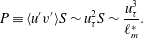 $$\begin{eqnarray}P\equiv \langle u^{\prime }v^{\prime }\rangle S\sim u_{\unicode[STIX]{x1D70F}}^{2}S\sim \frac{u_{\unicode[STIX]{x1D70F}}^{3}}{\ell _{m}^{\ast }}.\end{eqnarray}$$
Invoking the definition of turbulent diffusivity
 $\unicode[STIX]{x1D705}_{t}$
via the flux gradient relation, i.e.
 $$\begin{eqnarray}\unicode[STIX]{x1D705}_{t}\equiv -\frac{\langle \unicode[STIX]{x1D70C}^{\prime }v^{\prime }\rangle }{\text{d}\overline{\unicode[STIX]{x1D70C}}/\text{d}y},\end{eqnarray}$$
the buoyancy flux
 $B$
can be written as
 $B=-\unicode[STIX]{x1D705}_{t}N^{2}$
. Following the mixing length specifications (3.6) and (3.10), as well as the expression for
 $N^{2}$
in (A 2),
 $B$
can be rewritten as
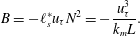 $$\begin{eqnarray}B=-\ell _{s}^{\ast }u_{\unicode[STIX]{x1D70F}}N^{2}=-\frac{u_{\unicode[STIX]{x1D70F}}^{3}}{k_{m}L}.\end{eqnarray}$$
As is shown in § 5, in figure 7 in particular, the flux Richardson number, defined as
 $Ri_{f}\equiv -B/P$
, is typically smaller than 0.2 in stratified plane Couette flows. One may make the further approximation
 $-B\ll P$
in (A 3), which results in the following scaling for
 $\unicode[STIX]{x1D700}$
:
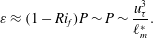 $$\begin{eqnarray}\unicode[STIX]{x1D700}\approx (1-Ri_{f})P\sim P\sim \frac{u_{\unicode[STIX]{x1D70F}}^{3}}{\ell _{m}^{\ast }}.\end{eqnarray}$$
Appendix B. Monin–Obukhov scaling: dimensionless quantities
The gradient Richardson number
 $Ri_{g}$
can be evaluated from (A 1) and (A 2):
 $$\begin{eqnarray}Ri_{g}\equiv \frac{N^{2}}{S^{2}}=\frac{u_{\unicode[STIX]{x1D70F}}^{2}}{k_{m}L\ell _{s}^{\ast }}\frac{\ell _{m}^{\ast 2}}{u_{\unicode[STIX]{x1D70F}}^{2}}=\frac{\ell _{m}^{\ast 2}}{k_{m}L\ell _{s}^{\ast }}.\end{eqnarray}$$
With
 $\ell _{m}^{\ast }$
and
 $\ell _{s}^{\ast }$
prescribed by Monin–Obukhov theory shown in (3.13),
 $Ri_{g}$
can be written as a function of the transformed wall-normal coordinate
 $\unicode[STIX]{x1D709}$
, i.e.
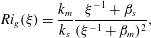 $$\begin{eqnarray}Ri_{g}(\unicode[STIX]{x1D709})=\frac{k_{m}}{k_{s}}\frac{\unicode[STIX]{x1D709}^{-1}+\unicode[STIX]{x1D6FD}_{s}}{(\unicode[STIX]{x1D709}^{-1}+\unicode[STIX]{x1D6FD}_{m})^{2}},\end{eqnarray}$$
where
 $k_{m}$
,
 $k_{s}$
,
 $\unicode[STIX]{x1D6FD}_{m}$
and
 $\unicode[STIX]{x1D6FD}_{s}$
are all dimensionless constants in Monin–Obukhov theory (§ 3.1).
We are particularly interested in the
 $Ri_{g}$
value at
 $y=0$
(
 $y_{w}=h$
or
 $\unicode[STIX]{x1D709}=h/L$
), a location characteristic of the midgap plateau as shown in figure 5. Such a characteristic
 $Ri_{g}$
value can be obtained by evaluating (B 2) at
 $\unicode[STIX]{x1D709}=h/L$
:
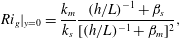 $$\begin{eqnarray}Ri_{g}|_{y=0}=\frac{k_{m}}{k_{s}}\frac{(h/L)^{-1}+\unicode[STIX]{x1D6FD}_{s}}{[(h/L)^{-1}+\unicode[STIX]{x1D6FD}_{m}]^{2}},\end{eqnarray}$$
an expression that has no explicit dependence on the Prandtl number
 $Pr$
. The influence of
 $Pr$
on the interior
 $Ri_{g}$
is indirect through the modulation of wall fluxes which determine the Obukhov length scale
 $L$
as defined in (1.1).
Combining (A 2) and (A 7), one can obtain an estimate for the buoyancy Reynolds number
 $Re_{b}$
:
 $$\begin{eqnarray}Re_{b}\equiv \frac{\unicode[STIX]{x1D700}}{\unicode[STIX]{x1D708}N^{2}}\sim \frac{u_{\unicode[STIX]{x1D70F}}L}{\unicode[STIX]{x1D708}}\frac{\ell _{s}^{\ast }}{\ell _{m}^{\ast }}k_{m}=L^{+}\frac{\ell _{s}^{\ast }}{\ell _{m}^{\ast }}k_{m}.\end{eqnarray}$$
As discussed in § 3.1, the ratio
 $\ell _{s}^{\ast }/\ell _{m}^{\ast }$
is typically of order unity, as prescribed by Monin–Obukhov theory. The above scaling (cf. Scotti & White Reference Scotti and White2016) thus becomes
 $$\begin{eqnarray}Re_{b}\sim L^{+}k_{m}.\end{eqnarray}$$
Following (A 4) and (A 6), the flux Richardson number
 $Ri_{f}$
can be estimated as
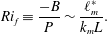 $$\begin{eqnarray}Ri_{f}\equiv \frac{-B}{P}\sim \frac{\ell _{m}^{\ast }}{k_{m}L}.\end{eqnarray}$$
With (B 1), the above scaling becomes
 $Ri_{f}\sim (\ell _{s}^{\ast }/\ell _{m}^{\ast })Ri_{g}$
. Again, with
 $\ell _{s}^{\ast }/\ell _{m}^{\ast }$
being
 $O(1)$
, one obtains
 $$\begin{eqnarray}Ri_{f}\sim Ri_{g},\end{eqnarray}$$
which is consistent with the observations of DCT (see e.g. their figure 13).
The other relevant parameter is the horizontal turbulent Froude number
 $Fr_{h}\equiv U^{\prime }/(\ell _{h}N)$
(e.g. Billant & Chomaz Reference Billant and Chomaz2001; Brethouwer et al.
Reference Brethouwer, Billant, Lindborg and Chomaz2007) which can be estimated by assuming
 $$\begin{eqnarray}\unicode[STIX]{x1D700}=\frac{{U^{\prime }}^{3}}{\ell _{h}}\end{eqnarray}$$
for the horizontal motions of the integral scale
 $\ell _{h}$
undergoing a forward cascade.
 $Fr_{h}$
can then be estimated as (see e.g. Maffioli et al.
Reference Maffioli, Brethouwer and Lindborg2016)
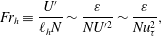 $$\begin{eqnarray}Fr_{h}\equiv \frac{U^{\prime }}{\ell _{h}N}\sim \frac{\unicode[STIX]{x1D700}}{N{U^{\prime }}^{2}}\sim \frac{\unicode[STIX]{x1D700}}{Nu_{\unicode[STIX]{x1D70F}}^{2}},\end{eqnarray}$$
for stratified plane Couette flows. Upon substituting (A 2) and (A 7) into (B 9), we obtain
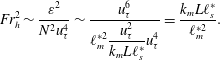 $$\begin{eqnarray}Fr_{h}^{2}\sim \frac{\unicode[STIX]{x1D700}^{2}}{N^{2}u_{\unicode[STIX]{x1D70F}}^{4}}\sim \frac{u_{\unicode[STIX]{x1D70F}}^{6}}{\displaystyle \ell _{m}^{\ast 2}\frac{u_{\unicode[STIX]{x1D70F}}^{2}}{k_{m}L\ell _{s}^{\ast }}u_{\unicode[STIX]{x1D70F}}^{4}}=\frac{k_{m}L\ell _{s}^{\ast }}{\ell _{m}^{\ast 2}}.\end{eqnarray}$$
Using (B 1), one obtains a scaling for
 $Fr_{h}$
as a function of
 $Ri_{g}$
:
 $$\begin{eqnarray}Fr_{h}\sim \frac{1}{\sqrt{Ri_{g}}}.\end{eqnarray}$$
Appendix C. Osborn formulation for the turbulent flux coefficient
The steady-state turbulent kinetic energy balance
 $P\approx \unicode[STIX]{x1D700}-B$
leads to
 $$\begin{eqnarray}-B\approx \frac{Ri_{f}}{1-Ri_{f}}\unicode[STIX]{x1D700}.\end{eqnarray}$$
Dividing the above equation by
 $\unicode[STIX]{x1D708}N^{2}$
and using
 $B=-\unicode[STIX]{x1D705}_{t}N^{2}$
,
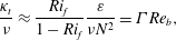 $$\begin{eqnarray}\frac{\unicode[STIX]{x1D705}_{t}}{\unicode[STIX]{x1D708}}\approx \frac{Ri_{f}}{1-Ri_{f}}\frac{\unicode[STIX]{x1D700}}{\unicode[STIX]{x1D708}N^{2}}=\unicode[STIX]{x1D6E4}Re_{b},\end{eqnarray}$$
where
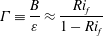 $$\begin{eqnarray}\unicode[STIX]{x1D6E4}\equiv \frac{B}{\unicode[STIX]{x1D700}}\approx \frac{Ri_{f}}{1-Ri_{f}}\end{eqnarray}$$
is the turbulent flux coefficient, and it is a fundamental question how
 $\unicode[STIX]{x1D6E4}$
(commonly referred to as ‘mixing efficiency’ in the oceanographic literature) is to be parameterized (see e.g. Ivey et al.
Reference Ivey, Winters and Koseff2008).