1. INTRODUCTION
1.1. Computerized design support
Building design within the field of architecture, engineering, and construction (AEC) is defined in this article as a process in which designers and engineers of many disciplines (e.g., architecture, structural design, mechanical, electrical, and plumbing engineering, and construction) cooperatively develop a description of a building to be constructed (the design solution) based on the project brief (the design requirements). In the past, this description was often a set of drawings, but it has evolved into three-dimensional (3-D) computer models as part of building information modeling (Eastman et al., Reference Eastman, Teicholz, Sacks and Liston2011). Building design can be regarded as coevolutionary, which means that both the design requirements and the design solution evolve cyclically (Maher, Reference Maher2000). Due to this coevolutionary character and the many disciplines involved, research has been carried out to investigate the applicability of computer tools that support the design team, for example, by providing design alternatives, including their predicted performance, and to study the design process itself. Related research that is relevant to this article will be presented in the following sections.
1.2. Data models
Data management is a very important aspect during a design process, and therefore data models have been developed for the spatial aspects of a building (Björk, Reference Björk1992; Borrmann & Rank, Reference Borrmann and Rank2009a, Reference Borrmann and Rank2009b), the structural design aspects (Weise et al., Reference Weise, Katranuschkov, Scherer, Goncalves, Steiger-Garcao and Scherer2000), and for the relation between spatial and structural design (Matthews et al., Reference Matthews, Duff, Corner, Sasada, Yamaguchi, Morozumi, Kaga and Homma1998). Although many research studies remain theoretically oriented, data models have also been implemented in computer design support tools (e.g., Scherer & Gehre, Reference Scherer, Gehre, Goncalves, Steiger-Garcao and Scherer2000; Mora et al., Reference Mora, Rivard and Bédard2008).
1.3. Automated facilities layout
Besides research on data models, many achievements have been made regarding computer programs, procedures, or concepts that generate solutions for spatial and structural design problems. Regarding spatial design, from the advent of computer-assisted design, space allocation, also known as automated facilities layout, has been a very important field of application. With space allocation, a building brief is transformed into a two-dimensional plan of the building (Ligget, Reference Liggett2000; Regateiro et al., Reference Regateiro, Bento and Dias2012), or more recently, into 3-D computer models. In addition, shape grammars, which use rules to transform geometrical elements into differently shaped elements, may be applied to develop spatial designs (Stiny, Reference Stiny2006; Turrin et al., Reference Turrin, Von Buelow and Stouffs2011).
1.4. Structural design optimization and generation
For structural design, a distinction should be made between the optimization of an existing structural design and the actual development (generation) of a structural design. Regarding optimization, different techniques can be used, including expert systems (Fuyama et al., Reference Fuyama, Law and Krawinkler1997), form-finding (Bletzinger et al., Reference Bletzinger, Wüchner, Daoud and Camprubi2005), topology optimization (Sigmund, Reference Sigmund2001), evolutionary structural optimization in which finite elements are deleted with low total strain values (Xie & Steven, Reference Xie and Steven1997), evolutionary computation (Rafiq, Reference Rafiq2000) and multidisciplinary grammars (Geyer, Reference Geyer2008). With regard to the actual development of a structural design, research has been reported that investigates the one-way transformation of a spatial design into a structural design. This concerns high-rise buildings (Maher, Reference Maher1985), the addition of structural grid lines to ground plans (Rafiq & MacLeod, Reference Rafiq and MacLeod1988), parametric templates (Sacks & Warszawski, Reference Sacks and Warszawski1997), shape annealing (Shea & Cagan, Reference Shea and Cagan1999), cased-based reasoning (Fenves et al., Reference Fenves, Rivard and Gomez2000), a sweep line algorithm coupled to an adjacency graph (Shaw et al., Reference Shaw, Miles and Gray2008), and assessing the performance of the design with respect to sustainability (Huang et al., Reference Huang, Breit and Mensinger2012).
1.5. Coevolutionary and multidisciplinary design
Most of the research presented above is carried out with the (implicit) assumption that the design requirements (i.e., spatial design properties) do not change. However, some research projects take into account that several disciplines strongly interact; that is, a discipline's interpretation of the design coevolves with all the other disciplines’ interpretations (Haymaker et al., Reference Haymaker, Fischer, Kunz and Suter2004). Inspired by this latter research work and related work on coevolutionary design (Maher, Reference Maher2000), a virtual toolbox has been implemented, which develops and modifies a spatial–structural building design through multiple cycles (Davila Delgado, Reference Davila Delgado2014). This virtual toolbox forms the basis on which the coevolutionary method as presented in this article has been developed. Although presented as generative design (see below), related research has been carried out on chair design, where topology optimization creates a chair skeleton, then this skeleton is modified spatially, and hereafter the resulting structure is again evaluated by structural analysis (Hemmerling & Nether, Reference Hemmerling and Nether2014).
1.6. Generative design
It is possible to use a set of rules to (most often automatically) generate design variants. For this, there needs to be a definition of the design space, rules to vary designs within this space, and evaluation methods to select the designs for further processing. The evaluation methods are based on manual selection or on sets of rules again (Krish, Reference Krish2011). A trade-off between the advancement of the set of rules and the level of scrutiny of the evaluation methods is studied by Königseder and Shea (Reference Königseder and Shea2014). Abrishami et al. (Reference Abrishami, Goulding, Rahimian and Ganah2014) integrate generative design with building information modeling. Genetic algorithms may be used within a generative design method to create the design variants, and at the same time, genetic algorithms themselves may be regarded as an overall method for generative design. In addition, the shape grammars mentioned in Section 1.3 can be regarded as components of generative design. Generative design is defined here as the recursive application of rules in initial designs, with the aim of creating designs variants, without emphasis on selection and evaluation. In this respect, for example, the work of Torghabehi and von Buelow (Reference Torghabehi, Buelow, Brazil and Pauletti2014) on the generation and evaluation of skin facades is regarded as generative design, whereas the interesting work of Hemmerling and Nether (Reference Hemmerling and Nether2014) is regarded as coevolutionary and multidisciplinary design (see above). Finally, activities exist that use parametric modeling of the building spatial design to support the design process in practice (Hesselgren et al., Reference Hesselgren, Charitou and Dritsas2007; Peters & Peters, Reference Peters and Peters2013), and these activities can be grouped either within “data models” (Section 1.2) or within this section.
1.7. Aim and contribution
The contribution of the research in this article is that existing, improved and newly developed procedures as found in the research above have been combined into a method that produces fully automatic 3-D spatial–structural coevolutionary building design cycles, an innovation not yet found in literature. Existing procedures are parametric templates (in this research defined as structural grammars), topology optimization, and evolutionary structural optimization, as presented in Section 1.4. New procedures have been developed for geometric redefinition, both for the building spatial design and the structural design, automatic stabilization, automatic loading, space deletion, and for the scaling and subdivision of a spatial design. The aims of this method are to support the building design process by providing optimized and coevolutionary generated design variants and to study the design process by investigating the influence of procedures on the coevolutionary process and its outcomes. This coevolutionary method has been compared with a genetic algorithm based method, the latter randomly varying these design variables of the spatial and structural designs that are also variable for the coevolutionary method.
1.8. Paper overview
Section 2 presents the coevolutionary method, followed by an explanation of the genetic algorithm based method in Section 3. In Section 4 the methods will be applied to two case studies, and the results will be discussed in Section 5. Finally, conclusions will follow in Section 6.
2. THE COEVOLUTIONARY METHOD
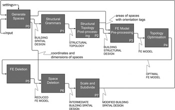
A coevolutionary method has been developed that follows an idealized real design process, in which building spatial and structural designs coevolve. As such, the method uses the procedures P0 to P7 as shown in the IDEF0 process model (National Institute of Standards and Technology, 1993) in Figure 1.
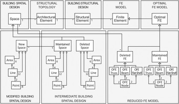
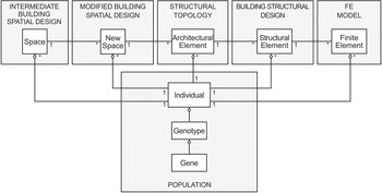
Each procedure will be briefly described below, and literature references will be provided for further details. Each class in the Unified Modeling Language (Booch et al., Reference Booch, Rumbaugh and Jacobson2005) data model (see Fig. 2) is capitalized in the text.
2.1. Generate spaces (P0)
This first procedure is used to generate a Building Spatial Design, which is based on text input of the width, depth, height, and position of spaces. Using basic calculations, each Space itself, and its Points for the eight corners are generated. As such, the procedure can be seen as a transformation from text input to objects (Spaces) stored in the data model. The reason it is defined as a separate procedure is that it can be extended with zoning (3-D pattern recognition), which enables the Building Spatial Design to be described by so-called zones, which are larger than individual Spaces (Hofmeyer & Bakker, Reference Hofmeyer and Bakker2008), but this description will not be used in this article.
IDEF0 process model of coevolutionary method.

Unified Modeling Language data model of the coevolutionary method.

2.2. Structural grammars (P1)
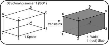
Based on the Building Spatial Design, the second procedure (P1) generates a Structural Topology, which is an assembly of Architectural Elements such as walls, columns, and slabs. The reason these are defined as Architectural Elements (and not Structural Elements) is that they do not yet have structural properties like Young's modulus and thickness and, in a real design process, they are often proposed by the architect, not the structural engineer. For the generation of the Structural Topology, structural grammars are used, which are partly inspired by shape grammars (Stiny, Reference Stiny1980; Knight, Reference Knight and Schmitt1992, Wang & Pinto Duarte, Reference Wang and Pinto Duarte2002; Kotsopoulos, Reference Kotsopoulos2008) and by methods to generate structural designs based on spatial designs (Rafiq & Macleod, Reference Rafiq and MacLeod1988; Sacks et al., Reference Sacks, Warszawski and Kirsch2000). The structural grammar used in this article is presented in Figure 3, where each Space serves as a template to add four Walls and one (roof) Slab.
Structural Grammar 1 (SG1).

2.3. Structural topology postprocessing (P2)
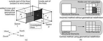
Once the Building Spatial Design is complemented with Architectural Elements, these elements form the Structural Topology. However, for the latter to become a Building Structural Design, several amendments have to be made. First, the Architectural Elements are provided with geometrical and material properties, and, consequently, are redefined as Structural Elements. Second, geometrical redefinition has to be performed (method A in Hofmeyer et al., Reference Hofmeyer, Van Roosmalen and Gelbal2011). Figure 4 illustrates the two reasons for geometrical redefinition and its concept: geometrical redefinition can be regarded as a procedure to remove the T-joints of Lines of Areas by rebuilding the geometry using additional Lines and Areas. This is applied to the Building Spatial Design, as shown in Figure 4a, to ensure an Area is either completely outside the building (and thus, e.g., should be loaded by wind load) or inside the building. Initially only Space 1 and Space 2 exist, and the Lines of the “investigated area” of Space 1 form T-joints with an Area of Space 2, which indicates that the investigated Area may be partly outside and partly inside the building. Note that in the figure, other Areas have also been split, which is indicated by “added Lines and Nodes after geometrical redefinition.” This is because all T-joints are automatically removed, even when this is not needed for appropriate loading later on. Geometrical redefinition is also applied to the Building Structural Design. Figure 4b shows that after redefinition, meshing of the finite element (FE) model results in coincident nodes, whereas coincident nodes are not guaranteed for a Building Structural Design that has T-joints.
Geometrical redefinition for (a) the Building Spatial Design for correct future loading and (b) the Building Structural Design for correct meshing of the finite element model.

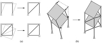
It cannot be expected that a Structural Topology, which is created by adding Architectural Elements to a Building Spatial Design, is stable naturally. However, it should be stable to ensure a useful and safe building and, more technically, to enable the FE model to be solved. Therefore, kinematic stabilization is carried out, as specified in Smulders and Hofmeyer (Reference Smulders and Hofmeyer2012), and shown by examples in Figure 5. A FE model is made from the Structural Topology. Note that this model (inside P2 in Fig. 1) should not be confused with the FE model to be used later on (between P3 and P4 in Fig. 1). Then, the so-called null space of the FE stiffness matrix is calculated, which gives complete information on which mechanisms in the Structural Topology occur. A structural element (Truss, Beam, or Flat-Shell) is added in an attempt to solve the first degree of freedom of the first mechanism. Then an updated finite element model is used to check this attempt. If the attempt is successful, then the addition will be kept; however, if no improved performance is detected, a different attempt will be carried out. This procedure will be followed until all mechanisms have been solved. For the case studies in Section 4, the procedure is set to add Flat-Shells as structural elements only, because this is most appropriate for the structural grammar used, which also uses Flat-Shells.
(a) Stabilizing different two-dimensional frames with a truss or additional constraints; (b) stabilizing a Building Structural Design using several trusses.

2.4. FE model preprocessing (P3)
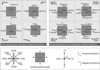
This P3 process transforms the Building Structural Design into an FE model, which enables the prediction of structural behavior (e.g., displacements, reaction forces, strains, and stresses) as a function of the loads applied. For the case studies in Section 4, a vertical live load case, a horizontal wind load case, and a combined case (using both previously mentioned cases) are used. The vertical live load case is defined by a downward directed, equally distributed load on every horizontal Flat-Shell of the Building Structural Design. The horizontal wind load is specified along one out of eight orthogonal or diagonal (nonorthogonal) directions, as shown in Figure 6. For wind in an orthogonal direction, pressure is applied to all “outside” (see Fig. 4) Areas of the Building Spatial Design that have their normal vector in the direction of the pressure. The same principle applies to Suction (0.8× value of pressure load) and Shear (0.4× value of pressure load), where the latter is applied to all outside Areas that have their normal vector perpendicular to the pressure direction. If a nonorthogonal direction for wind is preferred, the same load types are applied; however, now every Area is subject to two load types and all load values are divided by factor  $\sqrt{2}$ to take into account the diagonal direction of the wind.
Horizontal wind load definitions.

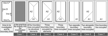
The loads defined on the Areas of the Building Spatial Design are transferred to the Structural Elements of the Building Structural Design via a weighted distribution. As shown in Figure 7, if a Flat-Shell (a Structural Element) is completely coincident with the Area investigated, the load is directly assigned to the Flat-Shell (Case 1). If all four Lines of the Area are occupied by either linear Structural Elements or by an edge of a Flat-Shell perpendicular to the Area (Case 2), areas A1 and A2 as shown in the figure are determined. Next, the load (N/mm2) is multiplied by the area A1 (mm2), divided by the length of line A (mm) and applied as line pressure to lines A and C. A similar procedure is carried out with A2 for lines B and D and for all other cases as well.
Cases for Structural Elements within an Area.

As a final step for this procedure, the Structural Elements are provided with a finite element mesh. For the case studies presented in this article, Flat-Shell Structural Elements are used, and they are mapped meshed with a four-node flat-shell structural element, for which its in-plane behavior is found in Cook et al. (Reference Cook, Malkus, Plesha and Witt2002), and its bending action conforms to the discrete Kirchoff triangular element developed by Batoz and Tahar (Reference Batoz and Tahar1982). The number of elements is determined by a factor D that prescribes the number of elements along the width and length of the Structural Flat-Shell Element. The flat-shell finite elements are assembled, and the resulting system of equations is solved via a biconjugate gradient stabilized solver for sparse square problems “BiCGSTAB”; see Guennebaud and Benoit (Reference Guennebaud and Benoit2014).
2.5. Topology optimization (P4)
After the FE model as developed in procedure P3 has been solved, strains and stresses can be predicted for each location in the Building Structural Design. If each finite element in the FE model was given a variable material density, it would be possible to locate more material (via a higher density) in highly strained and stressed regions in the design, removing this material from locations where only limited strains exist. This principle is known as Topology Optimization and was implemented in procedure P4 as follows (Sigmund, Reference Sigmund2001):
Step 1. Each element stiffness matrix is multiplied with a so-called relative density scalar, after which these element matrices are used to assemble the total system stiffness matrix.
Step 2. This system stiffness matrix and two columns for the nodal forces and displacements form a linear system of equations. This system of equations is solved, which results in predicted nodal displacements. Total strain energy can now be calculated as the sum over all elements of the product of the element stiffness matrix and the displacement vector found for this element.
Step 3. A derivation of this latter relation can be used to predict the sensitivity of the total strain energy for the variation of each element's relative density.
Step 4. The element sensitivities are used to assign improved element relative densities, with an added constraint that the average of the relative densities remains the same.
This process, given in Steps 1 to 4, is repeated until the change in relative densities (between Steps 1 and 4) is smaller than a predefined threshold. For multiple load cases, in Step 2 the system is solved for each load case and the total strain energies are summed up. Likewise, in Step 3, the sensitivities are summed up over all load cases as well. As a result, a Building Structural System is developed with Structural Elements having varying material density over their length, area, or volume.
2.6. FE deletion (P5)
To enable a more explicit interpretation of the Building Structural System and its material density found in the previous P4 procedure, in this P5 procedure finite elements with a low density are deleted. The elements are processed by the K-means algorithm (MacQueen, Reference MacQueen1967). This algorithm clusters the elements in a prescribed number of groups such that a minimal value exists for the sum over all groups of the sum in each group of the squared difference of the individual element value and the group average. Once these clusters have been formed, the deletion of finite elements is carried out by deleting a number of clusters that contain the elements with the lowest relative density values.
2.7. Space deletion (P6)
In a traditional design process, a Building Spatial Design influences the subsequent Building Structural Design. However, following the concept of coevolutionary design (Maher, Reference Maher2000), the Structural Design also influences the Spatial Design. In this article, an example of modeling the latter influence is given by procedure P6, which deletes Spaces at the locations where Finite Elements were deleted in the previous procedure. The rationale is that at locations where no structural mass is needed according to the optimization procedure, the Spaces present here could be positioned elsewhere, so the structural mass is not needed (to build the Spaces). After investigating how many deleted Finite Elements are coincident with the Areas of each Space, using Node and Point coordinates, the Space Deletion procedure functions as follows: the Spaces are ordered from the highest to lowest number of their associated removed finite elements; then a factor determines which part (e.g., 1/2, 1/3) of the ordered list is used (starting from the highest number) to delete the Spaces listed in this part.
2.8. Scale and subdivide (P7)
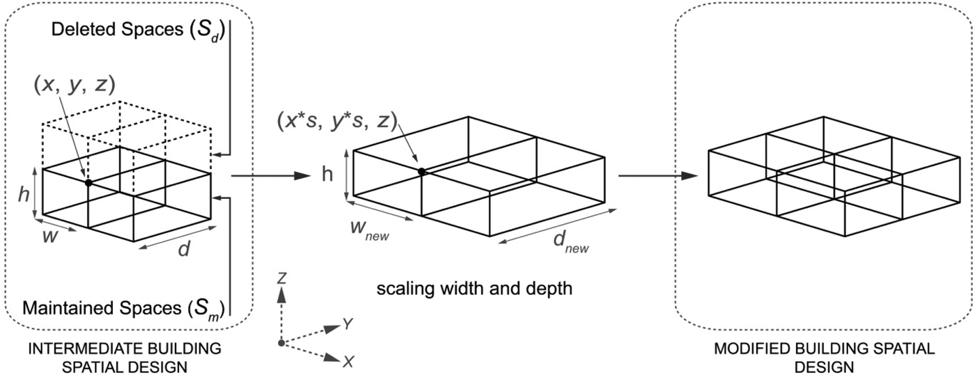
As the Building Spatial Design has been compromised in the previous procedure, because of the deletion of Spaces, it should be modified such that the original spatial requirements are fulfilled again. This is carried out in procedure P7 by scaling the complete Building Spatial Design such that its initial volume is restored. Because it is normally not very useful to scale the level height, only the width and depth are scaled, as shown in Figure 8 in the middle.
Scaling of the Intermediate Building Spatial Design.

Then, Spaces are split in order to restore the initial number of Spaces. If the number of deleted Spaces is higher than the number of maintained spaces, all maintained Spaces are split the same number of times, following a strategy to keep the ratio between the width and length of the new Spaces similar. If fewer deleted than maintained Spaces exist, very large Spaces are split such that the new spaces are the size of the smallest maintained Space. If this is not sufficient, Spaces are ordered in a list from their highest to their lowest volume, and starting with the highest volume, Spaces are each split into two new Spaces. If in this list maintained Spaces have the same volume, they are ordered using their x-coordinate, then the y-coordinate, and finally the z-coordinate. More details can be found in Davila Delgado (Reference Davila Delgado2014).
2.9. Coevolutionary cycles
The sequence of procedures P0 to P7, as shown in Figure 1, will lead to a cyclic method, in which Building Spatial Designs will be provided with a Building Structural Design. Then this structural design is improved (via topology optimization) and the spatial design is modified to take into account these structural improvements. Finally, certain requirements of the spatial design (e.g., volume and number of spaces) are restored, and hereafter the process starts again. As such, fully automatic 3-D spatial–structural coevolutionary building design cycles are carried out. In the next section, a genetic algorithm based method will be presented, which can then be used in comparison with the coevolutionary method.
3. GENETIC ALGORITHM BASED METHOD
3.1. Introduction
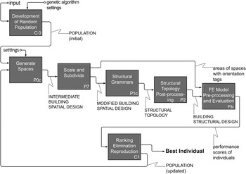
The coevolutionary method above generates accompanying building spatial and (optimized) structural designs using a method based on a human design process. Alternatively, in real life, constructed accompanying building spatial and structural designs can be regarded as the survivors among many designs that were created, however, were somehow not selected for construction. Using this principle, building spatial and (optimized) structural designs can be generated by a genetic algorithm based method presented in this section. Figure 9 presents an IDEF0 process diagram for the genetic algorithm based method, and Figure 10 shows the accompanying data model in Unified Modeling Language. Similar to the description of the coevolutionary method, every process will be briefly explained, and references will be given for more detailed information.
IDEF0 process diagram of the genetic algorithm based method.

Unified Modeling Language model of the genetic algorithm based method.

3.2. Development of random population (C0)
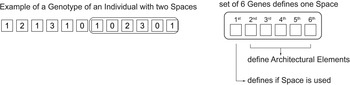
Based on the input (being equal to the input to the coevolutionary method) an initial population is developed, which consists of a number of Individuals, which is specified in the “genetic algorithm settings.” Each individual is represented by a Genotype, which consists of a string of digits (Genes)—six digits for each Space of the Individual—that contains all the necessary information for the generation of a Modified Building Spatial Design and a Building Structural Design, later on in the method. Figure 11 shows a Genotype of an Individual that will become a Building Spatial Design with two Spaces. The first six Genes are used for the first Space and the last six Genes for the second Space. In this example, both Spaces are used for the Building Spatial Design to be generated by processes P0c and P7, as the first gene is a “1” in both cases. The remaining five genes for every space determine the Building Structural Design, to be generated by processes P1c and P2, as further explained in Section 3.4. The C0 process generates the initial population by randomly filling the Genotypes with numbers.
Example of a genotype on the left; explanation of genes for 1 Space on the right.

3.3. Generate spaces (P0c)
The first part of this P0c process is equal to the P0 process of the coevolutionary method. Using the text file input of the building brief, listing all spaces with their width, depth, height, and position, instances of Space are generated with their eight corner points. The second part of the P0c process deletes each Space instance with its first gene equal to 0. To restore the total volume and number of Spaces, the P7 Scale and Subdivide process is used, exactly as described for the coevolutionary method: first the width and depth of the complete Building Spatial Design are scaled such that its initial volume is restored; and second, Spaces are split in order to restore the initial number of Spaces. For further details, please refer to Section 2.8 and Davila Delgado (Reference Davila Delgado2014).
3.4. Structural grammars (P1c)
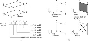
After the Building Spatial Design has been generated, it is provided with a Building Structural Topology via the “P1c Structural Grammars” procedure. The generated Genotype contains six genes for each Space of the Building Spatial Design. As explained, the first gene determines whether the Space will be used for the generation of the Building Spatial Design. The other five genes prescribe the Architectural Elements to be added to the six Areas of the Space, as shown in Figure 12. For example, the second Gene is associated with the Area with Points 1, 2, 7 and 6. This Gene received a random value of 0, 1, 2, or 3 during the development of the initial population. This now results in generating Architectural Elements, as shown in Figure 12 on the right. For example, if the random value equals 1, a single Wall will be positioned coincident with the Area given by Points 1, 2, 7 and 6.
Space with last five (out of six) Genes that indicate structural grammar 0, 1, 2, or 3 to be used (on the right) at Space Areas indicated by their four corner Points.

As described for the coevolutionary method already, process P2 (Structural Topology postprocessing) ensures the Building Structural Topology is transformed into a Building Structural Design by adding geometrical and material properties to the Architectural Elements, the application of geometrical redefinition, and the use of kinematic stabilization.
3.5. FE model preprocessing and evaluation (P3c)
This process follows process P3 as presented for the coevolutionary method. In addition, the total volume of all Structural Elements is determined via the Finite Elements to be used as a performance indicator.
3.6. Ranking, elimination, and reproduction (C1)
Out of the population, a number of randomly selected Individuals (the number given in the “genetic algorithm settings”) are ranked via a Pareto front according to their values of volume and total strain energy. A number (again given by the settings) of the lowest ranked Individuals is deleted, whereas the same number of highest ranked Individuals is used for reproduction via so-called crossover and mutation. Crossover implies that for two Individuals, each Genotype is split at (the same) random location, and Individuals exchange either the first or second part of their Genotype. For mutation, which is also applied to two Individuals at a time, both Genotypes are modified by randomly changing one Gene at a random location. The two newly generated Individuals are added to the population. A number of randomly selected individuals are taken, evaluated, ranked, and partly reproduced again; and this process is continued for a specified time period.
4. CASE STUDIES
4.1. Introduction
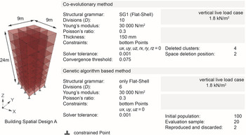
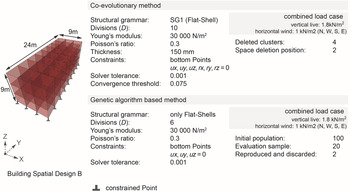
The coevolutionary and genetic algorithm based methods are both applied to two different Building Spatial Designs. The first design, named “A” and depicted in Figure 13, consists of eight levels 3 m in height, and each level contains 3 × 3 Spaces with dimensions of 3 × 3 m. It is loaded with the vertical live load case. The second design, named “B” and depicted in Figure 14, consists of three levels 3 m in height, with each level containing 3 × 8 Spaces with dimensions of 3 × 3 m. This design is loaded with the combined load case.
Building Spatial Design A, with settings for the coevolutionary and genetic algorithm based methods.

Building Spatial Design B, with settings for the coevolutionary and genetic algorithm based methods.

All settings used for the coevolutionary and genetic algorithm based methods are also listed in Figures 13 and 14. For the coevolutionary method, structural grammar SG1 (Flat-Shell) is used because the resulting shells for all space areas provide the largest design space to distribute structural mass for topology optimization. Consequently, to compare the coevolutionary method with the genetic algorithm, for the latter only Flat-Shells are used. For the Flat-Shells of the Building Structural Design, a thickness is used equal to 150 mm, and Young's modulus and Poisson's ratio are set equal to 30,000 N/mm2 and 0.3, respectively. The vertical live load is set to 1.8 kN/m2, and the horizontal wind load equals 1.0 kN/m2 for pressure (0.8 × 1.0 kN/m2 for suction and 0.4 × 1.0 kN/m2 for shear; see Section 2.4). Note that the vertical live load does not include the dead load, because the self-weight distribution changes considerably during topology optimization (process P4 in the coevolutionary method), and inclusion in this method would thus yield incomparable results with the genetic algorithm, which does not change the density distribution. For the coevolutionary method, where accurate finite element simulations are needed to correctly carry out topology optimization, 10 divisions (D, see Section 2.4) have been used, and this value is based on a mesh sensitivity analysis (Davila Delgado, Reference Davila Delgado2014). For the genetic algorithm based method, the finite element simulations are used to relatively rank the individuals only, and a trade-off between accuracy and computation time here leads to a division equal to 6. The solver tolerance applies to the finite element solver. It is the maximum allowable difference of the maximum term in the vector, which is the difference between the given load vector and the load vector obtained by substitution of the found displacement vector. A similar function is carried out by the convergence threshold, which ends the iterative topology optimization procedure if the largest change in relative density between two iterations is less than the threshold. The deleted clusters refer to four clusters (of eight) of finite elements to be deleted, whereas the space deletion position indicates that the ordered list of Spaces (from high to low number of deleted finite elements) is split into two equal parts, where subsequently the upper part is deleted.
Note that the actual implementation of the genetic algorithm based method makes use of Dexen, a so-called asynchronous decentralized approach, which is claimed to be scalable and robust (Janssen, Reference Janssen, Tidafi and Dorta2009). It implies that using the definitions of Janssen (Reference Janssen, Tidafi and Dorta2009) initialization (C0 in Fig. 9), development (P0c, P7, P1c, and P2), evaluation (P3c), and survival and reproduction (C1) are carried out independently and simultaneously by programs (called clients) on the population. A server allows or halts the requests of the clients to keep the population size constant. As such, the suggested workflow in Figure 9 is correct for understanding the method, but is technically an abstract representation.
Besides the case studies presented here, internal validation has also been carried out on the mesh sensitivity; the number of element divisions related to the number of deleted spaces; the relationship between the deleted clusters of finite elements and deleted spaces; the number of deleted spaces and the evolution of the spatial design; and high relative density locations. The internal validation is regarded as being too detailed to present here; however, it can be found in Davila Delgado (Reference Davila Delgado2014).
4.2. Results coevolutionary method for Building Spatial Design A
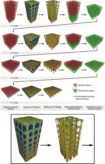
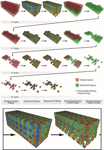
Figure 15 shows the results of the coevolutionary method for design A. Note that each row represents an iteration cycle of the method, whereas the columns show the outcomes of the procedures, as also given in Figure 2. It can be seen that the coevolutionary method causes a gradual reduction of the building height. This is because finite elements are strained less at the top of the building (due to fewer levels of live load above), and these elements are thus among the first to be deleted, causing the Spaces at these levels to be removed as well. Although more finite elements are removed at the top, the figure shows that at all levels sufficient elements are removed to enable a structural topology to show up. This structural topology suggests columns and slabs, naturally noninterfering with the Space interiors because there no Structural Elements have been placed, because of the structural grammar selected.
Coevolutionary method for Design A. Each row shows an iteration cycle; each column represents an indicated stage within the iteration cycle, close-up below.

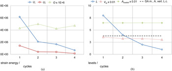
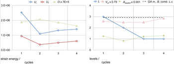
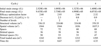
Table 1 lists the measurements for each cycle of the coevolutionary method. Total strain energies before (U i) and after topology optimization (U f) show that topology optimization is effective, and constantly so throughout the cycles, which is indicated by the efficacy optimization factor O (=U i/U f). This can also be seen in Figure 16 in the graph on the left, which also shows that Space Deletion (P6) and Scale and Subdivide (P7; indicated by the reduction of U i from Cycles 1 to 2) is almost as effective as topology optimization (indicated by the reduction of U i to U f in Cycle 1). Deleted spaces, spatial volume, and the number of spaces remain constant correctly, which is ensured by the Space Deletion (P6) and Scale and Subdivide (P7) processes, respectively. The structural volume is reduced due to the higher number of coincident vertical Space Areas for the Building Spatial Designs with fewer levels. Namely, although the structural grammar positions the same number of Architectural Elements in each Space (at the top horizontal and all vertical Areas), these Architectural Elements become Structural Elements later on in the process, and for coincident Space Areas only one and not two Structural Elements will be generated, thus reducing the number of Structural Elements for more coincident Areas.
Building Spatial Design A. Strain energy behavior is on the left (U i is the initial strain energy, U f is the final strain energy, O is the efficacy optimization factor); structural volume (V st), loaded area (A loaded), and number of levels (L) are on the right. The dotted line on the right is the average for the genetic algorithm (GA) based method.

Measurements for each cycle j of the coevolutionary method for spatial design A with a vertical load case

4.3. Results genetic algorithm based method for Building Spatial Design A
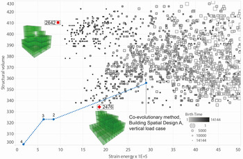
The genetic algorithm based method is illustrated in Figure 17 (coevolutionary results, indicated by the dotted line, are plotted for the discussion in Section 5). In total 2,696 Individuals have been developed, of which 2,615 have been evaluated for a Pareto frontier according to their values of volume and total strain energy (Davila Delgado, Reference Davila Delgado2014). However, for sake of clarity, only the Individuals with a strain energy of <50E5 have been shown. Every square indicates an Individual and the larger and lighter this square is, the older the Individual, that is, generated earlier in the simulation. As such, it can be seen that some later generated Individuals (smaller and darker) show a trend toward less strain energy. Among these Individuals, regarding structural volume, two groups seem to be formed, one at the upper region of the graph and one diagonally oriented in the middle. The lowest strain energy results from Individual 2,642, and its Building Spatial Design is included in the graph. In addition, the Building Spatial Design of Individual 2,476 is depicted, showing the least structural volume.
Genetic algorithm based method for Design A, 170 h, only strain energy <50E+5.

4.4. Results coevolutionary method for Building Spatial Design B
Figure 18 shows the results for the coevolutionary method for Building Spatial Design B. For this design, although now loaded with a combination of both vertical live and horizontal wind loads, the height of the building gradually decreases. In addition, the design shows horizontal fragmentation.
Coevolutionary method for Design B. Each row shows an iteration cycle; each column represents an indicated stage within the iteration cycle, close-up below.

After deletion of Finite Elements, the Reduced FE Model in Cycle 1 (Fig. 18) shows a structural topology of columns for the wide facade, including a diagonal brace at the corners, whereas the small facade is a shear wall without visible columns. This is due to the action of the wind load. Stability for the wind blowing in the building length direction is easily provided by the wide facade, thus allowing this facade to be optimized more for the vertical live load, resulting in columns, as seen for Design A as well. However, for wind blowing in the building width direction, the small facade needs material along its complete surface, dominating the columns that may have been visible otherwise.
Table 2 shows relevant measurements for the coevolutionary method. The total strain energies before (U i) and after topology optimization (U f) indicate that topology optimization is decreasingly effective, as shown by the efficacy optimization factor O (=U i/U f) and also in the left graph of Figure 19. Space Deletion (P6) and Scale and Subdivide (P7) in the first cycle (from U i in Cycle 1 to U i in Cycle 2) are shown to be equally effective as topology optimization (from U i in Cycle 1 to U t in Cycle 2). However, in all the following cycles, the Space Deletion and Scale and Subdivide processes result in increased total strain values because these processes cause the design to become fragmented and to have more external Space Areas. Because the wind load is defined to act on all external Space Areas, the total load increases, and thus (other variables remaining constant), total strain energy increases as well.
Building Spatial Design B. Strain energy behavior is on the left (U i is the initial strain energy, U f is the final strain energy, O is the efficacy optimization factor); structural volume (V st), loaded area (A loaded), and number of levels (L) on the right. The dotted line on the right is the average for the genetic algorithm (GA) based method.

Measurements for each cycle j of the coevolutionary method for spatial design B with a combined load case

Deleted spaces, spatial volume, and the number of spaces do not remain completely constant, because the Scale and Subdivide procedure (P7) will restore volume precisely; however, it is not always able to restore the number of Spaces exactly. For more details, see Davila Delgado (Reference Davila Delgado2014). The structural volume reduces by 4% after Cycle 1, remains constant for Cycles 2 and 3, and then increases by 14% for the last cycle. This last increase is caused by the fragmentation that results in more noncoincident vertical Space Areas, as explained before.
4.5. Results genetic algorithm based method for Building Spatial Design B
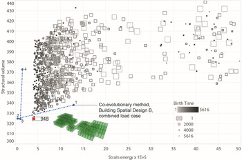
Figure 20 shows Building Spatial Design B used as input for the genetic algorithm based method. For this design 118 h of simulation time have been used, resulting in 1,060 Individuals developed and evaluated, but only those with a total strain energy of <50E + 5 have been shown for clarity. As was the case for Design A, some later generated Individuals (smaller and darker) show a trend toward less strain energy. However, among these Individuals, regarding structural volume, no trend can be determined because Individuals remain distributed over the height of the graph (the vertical axis indicating structural volume). A single Individual (948) shows both the lowest structural volume and total strain energy, and its Building Spatial Design has been visualized in Figure 20. It shows a similar reduction in height as for the coevolutionary method, and also fragmentation can be noticed. Both effects lead to a Building Spatial Design that is somewhat similar to the design in Cycle 3 of the coevolutionary method.
Genetic algorithm based method for Design B, combined load case, results after 118 h of simulation time, only individuals shown with strain energy of <50E + 5.

5. DISCUSSION
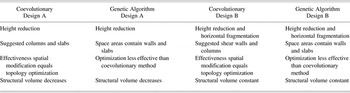
Table 3, which presents each case study, with the most important results in each column, shows that both methods, for both designs, show a significant reduced building height after the iterations. For the vertical live load of Design A, this is because finite elements are strained less at the top of the building (due to fewer levels of live load above), and these elements are thus among the first to be deleted for the coevolutionary method, causing the Spaces at these levels to be removed as well. The genetic algorithm based method shows similar behavior, however, because of random positioning of Spaces and Structural Elements and evaluation. For the combined load case of Design B, two explanations are possible. The first explanation is that wind loads have either no influence or promote the reduction of height as well, thus reinforcing the action of vertical load on height reduction. This seems to be a reasonable explanation because a lower building height results in less bending moment in the building due to the overturning wind load. In addition, when the building is lower with the same spatial volume, more volume is available for the transfer of forces coming from less vertical Areas loaded by winds. The second explanation is that the wind loads promote the increase of height, but then inevitably, the influence of the live load, as explained for Design A, is larger.
Case study results

For the combined load case, a second effect that can be observed for both methods is that the Building Spatial Design becomes fragmented. For the coevolutionary method, this is caused by deleted Spaces that are now located not only at the top of the building but also at other positions along the height, including the ground floor. Whereas a vertical live load results in more strain in the finite elements gradually from top to bottom, a combined case, especially the included wind load, results in overall bending of the building, straining the outer finite elements more than the elements at the building interior. Again, the genetic algorithm based method shows similar behavior due to the evaluation of random positioned Spaces and Structural Elements.
The topology optimization process in the coevolutionary method automatically yields suggestions for the building structural design. For a high-rise building with a vertical live load, a structure consisting of columns and slabs is suggested, whereas for a low-rise building with a combined load case, the columns are combined with shear walls. The genetic algorithm based method applies the structural grammar as shown in Figure 12 and thus shows a pattern with Space Areas containing a Wall or Slab.
As was shown in Sections 4.2 and 4.4, modification of the spatial design (via Space Deletion P6 and Scale and Subdivide P7) is as effective as topology optimization in optimizing the structural design. This is a surprising observation, as processes P6 and P7 have been developed intuitively, without the development of alternatives and comparisons, whereas topology optimization is a well-known and rigorous scientific method.
To compare the overall optimization performance of the two methods, the strain energy and structural volume for the four cycles of the coevolutionary method are plotted in Figures 17 and 20 as well. Because topology optimization is not used for the genetic algorithm based method, for the coevolutionary method, the total strain energy values are taken before topology optimization (U i), so topology optimization is also omitted. In addition, for the coevolutionary method, the total strain energy U i is taken from recalculated finite element simulations with D = 6, the same value that was used for the genetic algorithm based method, to make the comparison completely correct. For both designs and in general, the coevolutionary method arrives at lower total strain energy and structural volume in less time; however, it only generates four instead of many variants.
For the coevolutionary method for Design A, the structural volume is decreasing, as explained in Section 4.2. In addition, although the average structural volume over all individuals for the genetic algorithm as shown in Figure 16 on the right seems to be constant (because of the scale of the vertical axis), Figure 17 shows a reducing trend for both branches of individuals. For Design B, the coevolutionary method shows the constant structural volume (V st in Fig. 19), and the genetic algorithm based method does not converge to lower levels of structural volume but, as Figure 20 shows, forms a front with significant height.
Specifically for the coevolutionary method, it should be noted that it uses a single objective and the spatial design functions as a set of boundary conditions. Multiple-objective optimization could be carried out, for example, via parallel execution of coevolutionary cycles, each using the same spatial design but different objectives and “averaging” of the numerous modified spatial designs at the end of each cycle. This approach could also be used for handling the spatial design as a set of design variables (instead of boundary conditions). This is via optimizing the spatial and structural design in separate cycles, for example, by using a parametric description of the spatial design and “averaging” the designs at the end of both cycles.
The coevolutionary method is based on a human design process, whereas the genetic algorithm based method models evolution as found in nature. Thus, at first sight, it may seem surprising that for at least two different building designs, the optimal designs of both methods are similar (Table 3, rows 1 and 4). In contrast, both methods use the same optimization goal and design variables, so if they are capable of optimization, they should deliver the same solutions. What is surprising, though, is that the coevolutionary method, using quite an arbitrary procedure for spatial modification (processes P6 and P7), and using topology optimization that can only find local optima, still finds the same (or even better and faster) optimal designs as the other method, which carries out spatial modification randomly and can find global optima. Nevertheless, reducing the building height (and consequently increasing the ground plan area) may not be practical when taking into account the cost of the land, the building appearance, the natural view from the top stories, the functionality, and so forth. Likewise, both completely different methods indicate that for a combined load case, spatial designs become fragmented for more optimal structural designs. Again, this may violate the client brief in terms of functionality, architectural as well as client requirements. In conclusion, produced designs are comparable but may not be useful.
Taking the above principles of the two methods into account, how a human design process relates to design evolution in time is an interesting question. It is possible that designers have discovered “shortcuts” (the procedures in the coevolutionary method) to quickly arrive at currently used designs, these same designs matured for a long time, as seen from the perspective of evolutionary principles (as part of the genetic algorithm based method).
6. CONCLUSIONS
A coevolutionary method to explore accompanying building spatial and optimized structural designs has been developed. For this, new, improved, and existing procedures have been coupled to enable an automated cycle, in which 3-D spatial and structural designs coevolve, similar to a human design process. Design variables are varied systematically, and the topology optimization procedure is only able to find local minima.
For verification purposes, an existing genetic algorithm based method has been implemented, which uses exactly the same procedures as the coevolutionary method for spatial and structural design development and evaluation. Naturally for genetic algorithm based methods, design variables are varied randomly and global minima can be found.
Two building spatial designs have been used to compare the exploration and optimization of accompanying building spatial and structural designs for both methods. The coevolutionary method finds an optimal design (in this case, given the optimization criterion of minimal total strain energy) within a few cycles, thus producing only a limited number of variants. The genetic algorithm based method generates numerous variants; however, these variants only approach the optimum, even after a simulation time that is much larger than for the coevolutionary method.
The coevolutionary method has clearly shown that a human design strategy (e.g., “do not program spaces at locations where a structure is not needed”) has significant influence on the (modeled) design process, with different effects depending on the boundary conditions. For example, the strategy leads to reducing building height for a vertical live load, but in addition to fragmentation for a combined load. As such, the coevolutionary method can be used to test the effect of design strategies on the design outcomes and on the other design strategies involved.
As an overall conclusion, both methods can be used to find similar accompanying spatial and (optimized) structural designs and both are useful: the coevolutionary method to experiment with human design based strategies and the genetic algorithm based method to generate numerous design variants, which will avoid overlooking design possibilities not generated by the coevolutionary method.
The question that remains is how do the coevolutionary and genetic algorithm based methods relate philosophically? The coevolutionary method is similar to human design activities during design, whereas the genetic algorithm based method simulates design developments as seen in practice throughout history, without taking the design process into account, and following a trial and error process. Therefore, could the coevolutionary method be seen as a human created fast track, based on lessons learned from trial and error in the past?
Future research should incorporate the variation of all available settings, among which are the optimization of other design variables, the further variation of input and other selections of procedures, including further tuning of the genetic algorithm and the use of other search algorithms, such as Tabu Search (Glover, Reference Glover1989). Cases that can represent actual design problems should also be tackled.
Hèrm Hofmeyer is an Associate Professor at Eindhoven University of Technology. He received an MS in applied mechanics/design systems and a PhD in applied mechanics/steel structures from Eindhoven University of Technology. He was an invited visiting academic at Queensland University of Technology Brisbane for 3 months in 1998 and has worked at the University of Stuttgart, University of Liege, and RWTH Aachen University. One of Dr. Hofmeyer's recent research proposals was ranked first by the Dutch Technology Foundation STW, which allowed him to continue the research presented here with two new PhD students.
Juan Manual Davila Delgado is a Research Associate at the University of Cambridge Centre for Smart Infrastructure & Construction. He attained a BS in architecture at Tecnológico de Monterrey, an MS on a daylight respondent envelope design at Delft University of Technology, and a PhD at Eindhoven University of Technology. Dr. Delgado also worked on apartment design in architectural offices and for a short term at the National University of Singapore.