
1. Introduction
Traditionally, fixed-wing aircraft manoeuvres are performed by mechanically deflecting control surfaces, therefore altering the lift distribution of the aerodynamic surfaces and actuating control forces and moments. With increased expectations for aircraft economy, comfort, low observability and so on, it is extremely urgent to develop alternative flight control methods to improve the performance of aircraft. Among those existing controlling approaches, trailing edge circulation control (Wilde et al. Reference Wilde, Buonanno, Crowther and Savvaris2008; Crowther et al. Reference Crowther, Wilde, Gill and Michie2009; Smith & Warsop Reference Smith and Warsop2019; Warsop, Crowther & Forster Reference Warsop, Crowther and Forster2019) and fluidic thrust vector (Flamm et al. Reference Flamm, Deere, Mason, Berrier and Johnson2006; Ferlauto & Marsilio Reference Ferlauto and Marsilio2017; Li et al. Reference Li, Hirota, Ouchi and Saito2017) have gained increasing attention. The circulation control method can achieve roll control (Harley, Wilde & Crowther Reference Harley, Wilde and Crowther2009; Hoholis, Steijl & Badcock Reference Hoholis, Steijl and Badcock2016) or lift augmentation (Englar et al. Reference Englar, Hemmerly, Taylor, Moore, Seredinsky, Valckenaere and Jackson1981; Yubiao et al. Reference Yubiao, Liu, Yong, Lihua and Hong2018) by tangential blowing of air over the rounded trailing edge of a wing. Fluidic thrust vectoring, like circulation control, typically employs a rounded reaction surface to produce pitching and yawing moments (Mason & Crowther Reference Mason and Crowther2004; Li et al. Reference Li, Hirota, Ouchi and Saito2017; Warsop et al. Reference Warsop, Crowther and Forster2019) by deflecting the thrust of a jet engine without the need for mechanical devices. The efficiency of the circulation control is closely related to the jet velocity. Therefore, it is necessary to make the jet velocity supersonic by applying the circulation control method to aircraft control in transonic flights, and it is important to thoroughly understand the fluid mechanics of the supersonic jet over a convex wall.
The jet around a convex wall has two important flow developing regions, the inner boundary layer region near the curved surface and the outer shear layer region (Gnanamanickam et al. Reference Gnanamanickam, Bhatt, Artham and Zhang2019). There is not only the Tollmien–Schlichting-type viscous instability (Tsuji et al. Reference Tsuji, Morikawa, Nagatani and Sakou1977; Wernz & Fasel Reference Wernz and Fasel2007) in the inner part and the Kelvin–Helmholtz-type inflectional instability (Neuendorf & Wygnanski Reference Neuendorf and Wygnanski1999; Watanabe & Nagata Reference Watanabe and Nagata2021) in the outer part, both of which are active in the plane wall jet, but also Taylor–Görtler-type centrifugal instability (Görtler Reference Görtler1941; Cunff & Zebib Reference Cunff and Zebib1996; Matsson & John Reference Matsson and John1998) in the outer part owing to streamwise curvature caused by the Coanda effect (Henri Reference Henri1936). A series of previous studies has shown that this additional Taylor–Görtler instability plays an important role in the convex wall jet. Fujisawa & Kobayashi (Reference Fujisawa and Kobayashi1987) suggested that the significant increase of the convex wall jet spread and the levels of the Reynolds stresses along the downstream direction are rooted in the inviscid centrifugal instability. Neuendorf & Wygnanski (Reference Neuendorf and Wygnanski1999) and Likhachev, Neuendorf & Wygnanski (Reference Likhachev, Neuendorf and Wygnanski2001) confirmed that the turbulence intensity of the curved jet was significantly enhanced in comparison with the corresponding plane jet. Their later work observed the turbulent characteristics surrounding a pair of educed counter-rotating vortices, which suggested the existence of the streamwise vortices in the convex wall jet (Neuendorf, Lourenco & Wygnanski Reference Neuendorf, Lourenco and Wygnanski2004). Han, Zhou & Wygnanski (Reference Han, de Zhou and Wygnanski2006) used spanwise heterogeneities at the nozzle lip of a cylinder apparatus to force streamwise vortices, and found that these vortices were subsequently sustained by the centrifugal effects. In the latest work of Dunaevich & Greenblatt (Reference Dunaevich and Greenblatt2020), the spontaneously generated stationary streamwise structures were first observed using flow visualization and particle image velocimetry. These structures ultimately exhibited a secondary time-dependent wavy instability. Pandey & Gregory (Reference Pandey and Gregory2020) and Pandey & Gregory (Reference Pandey and Gregory2021) indicated that the centrifugal effect dominated the generation of the streamwise vortices, and the associated Eckhaus instability and the wavy instability were responsible for the increased turbulent stresses in the convex wall jet. However, all these studies focused on the low-speed incompressible convex wall jet rather than the compressible supersonic jet over a convex wall. Gregory-Smith & Gilchrist (Reference Gregory-Smith and Gilchrist1987) experimentally studied an under-expanded jet from a convergent slot and blowing over a convex curvature surface. The shadowgraph flow visualization showed that the shock cell structure disappeared more rapidly as the outer shear layer grew more quickly than that of a plane jet. They attributed this phenomenon to the destabilizing effect of the curvature on the turbulence in the shear layer. Later work of Gregory-Smith & Senior (Reference Gregory-Smith and Senior1994) in an axisymmetric model observed longitudinal streaks on the conical surface through surface oil flow visualization. As this feature was not seen in the planar model, this may suggest the existence of longitudinal Görtler-like vortices in the compressible jet over a convex wall. Recently, Wang, Wang & Zhao (Reference Wang, Wang and Zhao2017) experimentally investigated the convex curvature on the supersonic boundary layer. It was found that the convex curvature had significant impacts on the mean streamwise velocity and turbulent fluctuation, and these impacts were more influential in the outer layer. Sun, Sandham & Hu (Reference Sun, Sandham and Hu2019) and Wang et al. (Reference Wang, Wang, Sun, Yang, Zhao and Hu2019) used direct numerical simulation (DNS) to study supersonic turbulent flows over concave surfaces. Large-scale streaks and turbulence amplification, as well as Görtler-like vortices generated by the centrifugal effects, were observed. To sum up, numerous studies have confirmed that curvature has a significant effect on shear flow. However, in a supersonic jet over a convex wall, the existence of Görtler-like vortices has not been observed, and the role of these vortices in the shear layer instability is not clear either. Therefore, one of the motivations is to clarify the effect of centrifugal instability in the role of supersonic convex wall jet development.
In terms of the compressibility effect, most studies were carried out in the planar mixing layer. In order to evaluate the level of the compressibility in a mixing layer, the convective Mach number ( $M_c$), was defined by Papamoschou & Roshko (Reference Papamoschou and Roshko1988) and Bogdanoff (Reference Bogdanoff1983). For two gases with the same specific heat ratio, it can be expressed by
 $M_c=(U_1-U_2)/(a_1+a_2)$, where
 $U_1$,
 $U_2$ and
 $a_1$,
 $a_2$ represent the inflow velocities and local sound speeds for the two streams, respectively. Thanks to the advancements in numerical simulation and experiment methods, it has become feasible for researchers to better study shear layers with higher
 $M_c$ values. In numerous published numerical (Sandham & Reynolds Reference Sandham and Reynolds1991; Fu, Ma & Zhang Reference Fu, Ma and Zhang2000; Williams Reference Williams2003; Zhou, He & Shen Reference Zhou, He and Shen2012; Zhang, Tan & Li Reference Zhang, Tan and Li2017; Nagata, Watanabe & Nagata Reference Nagata, Watanabe and Nagata2018; Zhang, Tan & Yao Reference Zhang, Tan and Yao2019) and experimental studies (Papamoschou & Roshko Reference Papamoschou and Roshko1988; Clemens & Mungal Reference Clemens and Mungal1992; Hall, Dimotakis & Rosemann Reference Hall, Dimotakis and Rosemann1993; Elliott, Mo & Arnette Reference Elliott, Mo and Arnette1995; Urban & Mungal Reference Urban and Mungal2001; Goebel & Dutton Reference Goebel and Dutton2015; Kim, Elliott & Dutton Reference Kim, Elliott and Dutton2020), the trend of the decreasing the normalized shear layer growth rate with increasing
 $M_c$ has been widely recognized. The strong reduction in the compressible cases can be attributed to distinct compressibility effects. For weak compressibility condition (
 $M_c<0.4$), the instability was dominated by two-dimensional Kelvin–Helmholtz instability (Zhang et al. Reference Zhang, Tan and Li2017). For moderate compressibility condition (
 $0.4< M_c<0.8$), the dominant flow structure gradually changed from two-dimensional vortices to three-dimensional. At a higher compressibility condition (
 $M_c>0.8$), there was no curling and merging of vortex structures in the mixing layer (Elliott et al. Reference Elliott, Mo and Arnette1995). In the latest research of Kim et al. (Reference Kim, Elliott and Dutton2020), they used experimental methods to obtain the turbulent mixing layer development and turbulence stresses in the
 $M_c$ range from 0.19 to 0.88. It was confirmed that the normalized growth rate of the mixing layer reduces with increasing
 $M_c$. The turbulence measurements showed that the turbulence anisotropy increases with increasing compressibility. Above all, the compressibility effect has a significant influence on the development of the plane mixing layer. However, for the compressible shear layer over a convex wall, to the best of the authors’ knowledge, limited literature concerning this issue can be found. Gregory-Smith & Gilchrist (Reference Gregory-Smith and Gilchrist1987) and Gregory-Smith & Senior (Reference Gregory-Smith and Senior1994) experimentally studied the compressible jet over a convex wall. They found some evidence of a larger shear layer growth rate than that of a plane jet and the existence of streamwise vortices in the shear layer. The effect of different compressibility on the development of the shear layer has not been studied, and the mechanism of the influence of compressibility is still unclear. This is another motivation for the current work, to clarify the role the compressibility effect plays in the development of the supersonic convex wall jet.
Due to the existence of a boundary layer near the wall of the jet over a convex wall, high-fidelity simulations, such as DNS and large eddy simulation (LES) with the near-wall resolution, are extremely expensive. For example, a recent DNS by Naqavi, Tyacke & Tucker (Reference Naqavi, Tyacke and Tucker2018) of a jet Reynolds number  $Re_j=U_jh/\nu =7200$ (where
 $h$ is the slot height,
 $U_j$ is the jet slot exit velocity and
 $\nu$ is the kinematic viscosity) plane wall jet, employed
 $1652 \times 344 \times 302$ grid points in the streamwise, wall-normal and spanwise directions, respectively, which results in approximately 172 million cells. However, for the supersonic jet in the current study,
 $Re_j=U_jh/\nu =218\ 000$ (based on the sound speed), which is at least 30 times that of Naqavi et al. (Reference Naqavi, Tyacke and Tucker2018). The huge amount of grids caused by the high Reynolds number (
 $N\sim Re^{9/4}$, where
 $N$ presents the number of grids) (Moin & Mahesh Reference Moin and Mahesh1998) makes the expensive computational consumption unaffordable. Since this study mainly focuses on the development of the shear layer in the outer region of the jet, one approach to saving the computational cost is the use of the detached-eddy simulation (DES) method. The DES method is the hybrid of a Reynolds-averaged Navier–Stokes (RANS) calculation and LES which attempts to reduce the cost of LES by employing RANS in boundary layers (Spalart et al. Reference Spalart, Deck, Shur, Squires, Strelets and Travin2006). Therefore, the delayed detached-eddy simulation (DDES) method developed from the DES method is adopted to study the supersonic jet over the convex wall in this paper. In addition, a widely applicable data-driven modal decomposition method, dynamic mode decomposition (DMD) (Schmid & Sesterhenn Reference Schmid and Sesterhenn2010), is employed to decompose the flow field and gain further insight into the dynamical behaviours.
This paper is organized as follows: § 2 describes the details of the numerical methods. In § 3, computational details are described. Numerical results and analysis are presented in § 4. The last section contains the main conclusions.
2. Numerical methods
2.1. Delayed detached-eddy simulation
The basic governing equations are the RANS equations. For the additional Reynolds stress in the RANS equations, researchers have constructed many turbulence models to solve it. The shear-stress transport (SST) (Menter Reference Menter1994) turbulence model is adopted in this paper.
The two-equation SST DDES method is implemented by modifying the dissipation-rate term of the turbulent kinetic energy transport equation as follows:
 $$\begin{gather} \frac{\partial ({\rho k})}{\partial t}+\frac{\partial ({\rho U_i k})}{\partial x_i}=\widetilde{P_k}-\frac{\rho k^{3/2}}{l_{hybrid}}+\frac{\partial }{\partial x_i} \left[(\mu+\sigma_k\mu_t ) \frac{\partial k}{\partial x_i}\right], \end{gather}$$
 $$\begin{gather}\frac{\partial ({\rho \omega })}{\partial t}+\frac{\partial ({\rho U_i \omega})}{\partial x_i}=\frac{\gamma }{\nu_t }\widetilde{P_k}-\beta\rho\omega^2+\frac{\partial }{\partial x_i} \left[(\mu+\sigma_{\omega }\mu_t ) \frac{\partial \omega}{\partial x_i}\right]+2 (1-F_1 )\rho\frac{\sigma _{\omega2}}{\omega}\frac{\partial k}{\partial x_i}\frac{\partial \omega}{\partial x_i}, \end{gather}$$
where  $\rho$ is the density,
 $\mu$ is the viscosity,
 $\gamma$ is the specific heat ratio,
 $\sigma_k$ and
 $\sigma_\omega$ are diffusion coefficients of k and
 $\omega$,
 $P_k$ is the production term of turbulent kinetic energy,
 $k$ and
 $\omega$ represent the turbulent kinetic energy and specific dissipation rate, respectively,
 $\beta$ is a constant and the value of
 $\beta$ is recommended as 0.09 by Menter (Reference Menter1994). Also,
 $l_{hybrid}$ is the length scale defined as
 $$\begin{gather} l_{hybrid}=min\{ l_{RANS},l_{LES} \}, \end{gather}$$
 $$\begin{gather}l_{RANS}=\frac{k^{1/2}}{\beta\omega}, \quad l_{LES}=C_{DES} \varDelta=C_{DES}max \{{\varDelta_x,\varDelta_y,\varDelta_z} \}, \end{gather}$$
in which  $l_{RANS}$ and
 $l_{LES}$ are the length scales of the RANS turbulence model and LES method, respectively. Here,
 $\varDelta$ is the grid scale, which is equal to the maximum grid spacing in the
 $x$,
 $y$ and
 $z$ directions for the structured grid,
 $C_{DES}$ is an empirical constant that needs to be calibrated and verified, reflecting the degree of dissipation in different computational fluid dynamics (CFD) codes. As for the SST turbulence model,
 $C_{DES}= ( 1-F_1 )C_{DES}^{outer}+F_1C_{DES}^{inner}$, where
 $C_{DES}^{outer}$ is equal to 0.61,
 $C_{DES}^{inner}$ is equal to 0.78 and
 $F_1$ is the internal function (Spalart et al. Reference Spalart, Deck, Shur, Squires, Strelets and Travin2006) in the SST turbulence model.
However, within the DES method exists modelled-stress depletion which will produce the grid induced separation. To overcome this problem, Spalart et al. (Reference Spalart, Deck, Shur, Squires, Strelets and Travin2006) proposed a new method, named DDES, by constructing a delayed function. The length scale of DDES can be expressed as follows:
 \begin{equation}
\left. \begin{array}{@{}c@{}} l_{hybrid}=l_{RANS}-f_dmax\{
0,l_{RANS}-l_{LES} \}\\
f_d=1-\tanh[ ( 8r_d )^3 ]\\
\displaystyle r_d=\dfrac{\nu+\nu_t}{\sqrt{u_{i,j}u_{i,j}}\kappa^2 d^2}
\end{array}\right\},\end{equation}
where the  $f_d$ is the delayed function,
 $\nu _t$ is the kinematic eddy viscosity,
 $\nu$ is the molecular viscosity,
 $u_{i,j}$ are the velocity gradients,
 $\kappa$ is the Kármán constant of 0.41 and
 $d$ is the distance to the wall. The structure of the delay function and the meaning of the parameters are detailed in Spalart et al. (Reference Spalart, Deck, Shur, Squires, Strelets and Travin2006). In the case
 $f_d$ tends to 0, RANS calculation is used. And in the case
 $f_d$ tends to 1, the DDES method is converted to the traditional DES method.
2.2. Numerical issues
Spatial discretization resolution is critical for a high-fidelity numerical simulation. To level down the numerical dissipation, the inviscid fluxes are computed via a Roe flux-difference upwind scheme with a fifth-order weighted essential non-oscillatory scheme (Liu, Osher & Chan Reference Liu, Osher and Chan1994). The viscid fluxes are discretized by a fourth-order central differencing scheme. The fully implicit lower upper-symmetric Gauss–Seidel (time-marching scheme (Yoon & Jameson Reference Yoon and Jameson1988) with a second-order dual time-stepping method and Newton's sub-iteration for the inner loop is employed for time marching to achieve unsteady simulation.
In order to accelerate the formation of unsteady turbulent motions, all unsteady DDES simulations were initialized with corresponding converged steady RANS solutions. The unsteady DDES calculations are implemented with a fixed physical time-step size of  $1.44\times 10^{-7}$ s. A maximum of 10 sub-iterations per time step were used, resulting in a residual drop of at least 2–3 orders. After the transient flow with 25 000 steps, the remaining 8000 steps are taken to obtain sufficient unsteady flow data per 25 steps for statistical analysis. The total physical time of 8000 steps allows the fluid to flow over 2.5 times the arc length of the convex wall at the characteristic velocity (sound speed) to ensure that the periodic motions of the typical coherent structures can be effectively captured.
2.3. Dynamic mode decomposition
Modal analysis methods are becoming more and more popular in the analysis of flow mechanisms (Rowley & Dawson Reference Rowley and Dawson2017; Taira et al. Reference Taira, Brunton, Dawson, Rowley, Colonius, Mckeon, Schmidt, Gordeyev, Theofilis and Ukeiley2017, Reference Taira, Hemati, Brunton, Sun and Yeh2020). Among these methods, The DMD is a flow field decomposition method that can decompose flow field modes with different frequencies and realize the flow field evolution of each mode. It is the singular value decomposition variant proposed by Schmid & Sesterhenn (Reference Schmid and Sesterhenn2010). A given set of flow field snapshots, equispaced in time, are rearranged into a data matrix
 \begin{equation} \left. \begin{array}{@{}c@{}} X=[ x_1,x_2,x_3,\cdots ,x_{N-1} ]\\ Y=[ x_2,x_3,x_4,\cdots ,x_{N} ] \end{array}\right\}.\end{equation}
We assume that two different snapshots can be represented in a linear manner
 \begin{equation} x_{i+1}=A\cdot x_i. \end{equation}
Therefore, the two flow field snapshot matrices can be expressed as follows:
 \begin{equation} \left. \begin{array}{@{}c@{}} Y=[ x_2,x_3,x_4,\cdots ,x_{N} ]\\ =[ Ax_1,Ax_2,Ax_3,\cdots ,Ax_{N-1} ]\\ =AX \end{array}\right\}.\end{equation}
The singular value decomposition of the flow field snapshot matrix  $X$ is as follows:
 \begin{equation} X=U \varSigma V^T, \end{equation}
where the shape of the matrix  $X$ is assumed as
 $m\times (N-1)$, the matrix
 $\varSigma$ is the
 $r$-order diagonal matrix. Therefore, the shapes of the matrix
 $U$ and
 $V$ are
 $m\times r$ and
 $(N-1)\times r$, respectively.
A similar transformation of matrix  $A$ is realized by utilizing the matrix
 $U$. The
 $m$-order matrix
 $A$ is reduced to the
 $r$-order matrix
 $\tilde {A}$. Therefore, the similarity matrix
 $\tilde {A}$ can be solved as follow:
 \begin{equation} \tilde{A}=U^T A U =U^TYV \varSigma^{{-}1}. \end{equation}
The matrix  $\tilde {A}$ is the low-dimensional approximation of the matrix
 $A$. Tu et al. (Reference Tu, Rowley, Luchtenburg, Brunton and Kutz2014) have shown that
 $\tilde {A}$ includes the main eigenvalues of
 $A$. Eigenvalue
 $\mu _j$ and eigenvector
 $w_j$ can be solved by
 $\tilde {A}y_j=\mu _jw_j$. The DMD mode is defined as
 \begin{equation} \varPhi_j=Uw_j. \end{equation}
The matrix  $A$ is related to
 ${\rm \Delta} t=t_{j+1}-t_j$. Hence, stability information can be related by the logarithmic mapping of
 \begin{equation} \lambda _j=\frac{\log( \mu_j )}{{\rm \Delta} t}, \end{equation}
where the real and imaginary components of  $\lambda _j$ contain the growth rate and the frequency of the DMD mode. Besides, the order of the DMD modes is sorted by comparing the values of amplitudes
 $\| \varPhi _j \|$ with rank the contributions to the overall energy.
3. Computational details
3.1. Model, flow conditions and boundary conditions
An apparatus including a convergent–divergent nozzle and a curved Coanda surface was examined in this study. The geometric design method of the convergent–divergent nozzle is a quasi-one-dimensional method based on isentropic flow theory without boundary layer corrections. This method does not provide any other geometric shape information about the nozzle except the area ratio of the throat and exit for a given design point pressure ratio. In the design of the nozzle shape, the geometric tangency of the positions (i.e. the throat, the connection between the nozzle exit and Coanda surface), where the area changes, is ensured to eliminate the influence of geometric mutation on the flow. In addition, a symmetrical shape of the nozzle is employed to avoid geometrically induced non-uniform flow at the jet outlet. The nozzle exit height is 10 mm, and the design point of the nozzle pressure ratio is 7 ( $NPR_d = 7$). The Coanda surface is a
 $90^{\circ }$ circular arc with a radius of
 $100$ mm, fixing the
 $h/R$ ratio to 0.1. Experiments were conducted by Llopis-Pascual (Reference Llopis-Pascual2017) at the University of Manchester. They obtained the pressure coefficient distribution of the Coanda surface and the Schlieren photograph of the jet. Unfortunately, no turbulence statistics of the jet were measured. As the experiments were carried out in quiescent air, the test conditions were
 $p_{amb}=100$ kPa and
 $T_{amb}=300$ K.
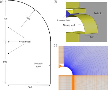
The computational domain and boundary conditions are shown schematically in figure 1. Since the experiment device was fixed on a wall, the no-slip wall boundary conditions are applied at the side of the jet inlet. The pressure outlets ( $p/p_{amb}=1$) are employed for the other far boundary. Periodic boundary conditions are applied in the spanwise direction. The inlet of the jet plenum is set to be the pressure inlet, where the nozzle pressure ratio is specified (
 $p/p_{amb}=NPR, T/T_{amb}=1.2$) and p and T represent pressure and temperature at pressure inlet, respectively.
Schematics of (a), (b) computational domain and boundary conditions, and (c) grid around the curved wall.

The basic geometric characteristics of the device and the cylindrical coordinate axes employed in this study are shown in figure 2. Azimuthal ( $\theta$), radial (
 $y$) and spanwise (
 $z$) coordinates correspond to the
 $U$,
 $V$ and
 $W$ components of velocity, respectively. The jet half-width (
 $y_2$), which is the wall-normal location where the streamwise velocity is half (
 $0.5U_{max}$) of its maximum value, is used as a measure of the jet thickness.
Schematics of the coordinate system.

3.2. Computation validation and grid sensitivity
3.2.1. Computation validation
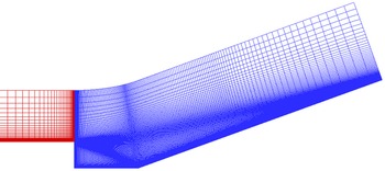
All numerical simulations in this study were conducted using an in-house three-dimensional cell-centred finite volume solver developed by the authors. The solver has been successfully applied to numerical studies on subsonic flows (Qu & Sun Reference Qu and Sun2017), supersonic flows (Qu et al. Reference Qu, Sun, Han, Bai, Zuo and Yan2019b; Sun et al. Reference Sun, Qu, Liu, Yao and Bai2020) and hypersonic flows (Sun, Qu & Yan Reference Sun, Qu and Yan2018; Qu et al. Reference Qu, Chen, Sun, Bai and Zuo2019a). Also, Mach 2.92 past a ramped cavity configuration (Baca Reference Baca1982; Hayakawa, Smits & Bogdonoff Reference Hayakawa, Smits and Bogdonoff1984) is presented for the solver validation. Figure 3 depicts a schematic cross-section of the experimental arrangement as well as the experimental locations of the velocity and turbulence fluctuation profiles. The numerical simulations in this research are carried out using grids of the same scale as those used in Reference Fan, Xiao, Edwards, Hassan and BaurleFan et al.'s (Reference Fan, Xiao, Edwards, Hassan and Baurle2004) numerical investigation of the same set-up. Figure 4 shows the centreplane grid of the configuration. The grid consists of two blocks, with  $41\times 56\times 33$ points upstream of the cavity (red) and
 $166\times 156\times 33$ points downstream of the leading edge of the cavity (blue). The grid extends
 $0.0381$ m in the spanwise direction. The initial grid distance from the wall is
 $3\times 10^{-6}$ m to keep
 $y^+\sim O(1)$ .
Cross-section of experimental configuration (from Baca Reference Baca1982).

Centreplane grid for ramped cavity configuration.

The nominal flow Mach number, temperature and unit Reynolds number are  $2.92$,
 $95K$,
 $6.7\times 10^7\ \textrm {m}^{-1}$, respectively. The upstream flat plane is adjusted to ensure that the velocity profile at
 $x=-25.4$ mm matches the experimental value. The converged steady RANS solution is used as the initial of unsteady DDES simulation. A fixed time step of
 $1.5\times 10^{-7}$ s is used for the calculation, and ten subiterations are required to reduce the residual at each physical time step by at least two orders of magnitude. The first 30 000 time steps are employed to establish a statistically stationary state, and then statistics are gathered for the additional 20 000 time steps.
Figure 5 shows a comparison of the measured by Baca (Reference Baca1982) and computed mean velocity profiles in the shear layer at three streamwise stations indicated in figure 3. The mass flux fluctuations in the shear layer were experimentally measured by Hayakawa et al. (Reference Hayakawa, Smits and Bogdonoff1984). The corresponding profiles extracted from the DDES computations are presented in figure 6. The results are in good agreement with the experiments made by Baca (Reference Baca1982) and Hayakawa et al. (Reference Hayakawa, Smits and Bogdonoff1984). In the shear layer, the solver utilized in this research has high solution accuracy.
Mean velocity profiles in the shear layer. Experimental data from Baca (Reference Baca1982) (Exp–Baca); (a)  $x/D=1.5$, (b)
 $x/D=2.5$ and (c)
 $x/D=3.5$.

Mass flux fluctuations in the shear layer. Experimental data from Hayakawa et al. (Reference Hayakawa, Smits and Bogdonoff1984) (Exp–Hayakawa); (a)  $x/D=1.5$ and (b)
 $x/D=2.5$.

3.2.2. Grid sensitivity
Two mesh sizes were used to characterize the grid dependence of the solution. The coarse mesh contains  $N_{\theta }\times N_y\times N_z=251\times 151\times 121$ grids around the convex surface (resulting in a total of 6.6 million grids), while the fine mesh has
 $N_{\theta }\times N_y\times N_z=301\times 171\times 151$ grids around the convex surface (resulting in a total of 10.5 million grids). The grids in the
 $y$-direction are refined near the convex surface and the jet shear layer to accurately trace the boundary layer and the complex vortex development, respectively. In the
 $\theta$ and
 $z$ directions, the grids are uniformly spaced. The first grid spacing from the convex wall is chosen to ensure that
 $y^+<1$ (
 $y^+=\rho _wU_{\tau \cdot w}y_{wall}/\mu _w$, where
 $y_{wall}$ is the height of the first grid from the wall,
 $U_{\tau \cdot w}$ is the local friction velocity,
 $\rho _w$ and
 $\mu _w$ are the local wall density and viscosity).
Figure 7 presents the mean Mach contours for both the coarse and fine grids. The coarse grid results are shown as colour contours, while the fine grid results are shown as black lines. Figure 8 depicts the ensemble- and spanwise-averaged streamwise velocity distributions (normalized by ambient air sound speed) at various streamwise locations. Figure 9 shows the jet development along the downstream location by displaying the jet half-width and vorticity thickness of the shear layer. The results obtained with the two meshes demonstrate excellent grid independence.
Effect of grid resolution on mean flow structure: coarse (colour contours), and fine grid (black lines).

Ensemble- and spanwise-averaged streamwise velocity distribution from  $\theta =0^{\circ }$ to
 $90^{\circ }$; (a)
 $0^{\circ }$, (b)
 $25^{\circ }$, (c)
 $45^{\circ }$, (d)
 $65^{\circ }$ and (e)
 $90^{\circ }$.

Ensemble- and spanwise-averaged (a) jet half-width and (b) vorticity thickness of the jet shear layer.

It should be noted that the original vorticity thickness formula is  $\delta _{\omega }={\rm \Delta} U/ | \textrm {d}u/{\textrm {d} y} |_{max}$. The formula is defined in the plane mixing layer. Different from the plane mixing layer, the mainstream velocity of the jet over a convex wall changes significantly as the jet develops downstream (figures 12a and 13a). Therefore, to consider the effect of the velocity variation,
 ${\rm \Delta} U$ is calculated by the local maximum streamwise velocity in this study.
In addition, the grid independence of the fine mesh will be demonstrated by the following three aspects. Firstly, for reliable DDES simulations, the grid size has to be adequately small to resolve the desired turbulent structures. The smallest Kolmogorov scale  $\eta = (\nu ^3 \varepsilon )^{1/4}$ is estimated as approximately
 $0.04$ mm in the jet mixing layer centre for the present simulations; here,
 $\nu$ and
 $\varepsilon$ are the kinematic viscosity (calculated by Sutherland's law) and turbulent kinetic energy dissipation rate (estimated by
 $RNG\ k{-}\varepsilon$ model), respectively. The grid spacings around the jet mixing layer in the
 $( \theta,y,z )$ directions are specified as
 $(0.52, 0.05, 0.67)$ mm, which are approximately
 $(12.5, 1.25, 17)$ times the Kolmogorov scale and are fine enough to resolve the jet mixing layer. Secondly, the computation domain in the
 $z$ direction should be sufficiently wide to capture enough spanwise flow structures. The instantaneous visualization of vortex structures using
 $Q$-criterion (the variable Q is defined as the second invariant of the velocity gradient tensor) and the ensemble average of the streamwise vorticity at
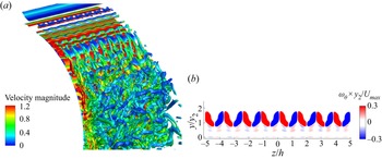
 $\theta =25^{\circ }$ are shown in figure 10. It can be seen that the spanwise flow periodicity is well captured and the spanwise scale in the present simulation is reasonable. Furthermore, the numerical pressure coefficient distribution on the Coanda wall agrees with the experiment of Llopis-Pascual (Reference Llopis-Pascual2017) well (figure 11). This further proves the accuracy of the grid and solver in the present study. Thus, the resolution of fine mesh is considered to be sufficient for the unsteady numerical simulation and will be utilized in all of the present investigations.
Spanwise flow structure resolution, (a) instantaneous visualization of vortex structures using  $Q$-criteria (
 $Q=100$), (b) ensemble average of streamwise vorticity
 $\theta =25^{\circ }$.

Comparison of pressure coefficient along the Coanda surface ( $NPR=3.0$, experimental results: Llopis-Pascual Reference Llopis-Pascual2017).

4. Results and discussion
In this section, numerical simulations are carried out to explore the dynamics of the supersonic jet over a curved wall in the current study. Here, the nozzle pressure ratio of  $3.0$ is employed as the basic case; all analyses in this section are based on this case unless otherwise stated. Firstly, the basic features of jet development are studied. Secondly, the basic case is employed to analyse the generation of the streamwise vorticity and its role in the development of the jet. Thirdly, the turbulent fluctuation evolution is investigated. Finally, the influence of the compressible effect is investigated with different convective Mach numbers.
4.1. Basic features of supersonic convex wall jet development
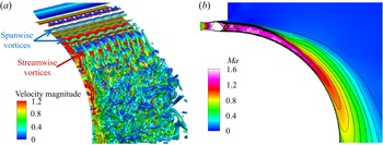
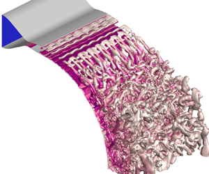
At the initial stage of jet development, spanwise vortices are generated in the shear layer under the dominance of Kelvin–Helmholtz instability. Subsequently, the role of streamwise vortices gradually becomes prominent. The existence of streamwise vorticity will cause the skewness of the spanwise vorticity and accelerate the instability of the shear layer. With the instability of the shear layer, the large-scale vortex structure is broken into smaller-scale vortices (figure 12a). This indicates that the turbulence intensity increases, in other words, the momentum exchange capacity of the shear layer is enhanced. Figure 12(b) shows the ensemble- and spanwise-averaged Mach number contours of the jet; as the jet develops downstream, the shear layer thickness increases while the mainstream velocity decreases gradually under the effect of viscosity and shear layer entrainment.
Development of the compressible jet over a convex wall; (a) instantaneous overall visualization of the vortex structures using  $Q$-criteria for the jet (
 $Q=100$), (b) ensemble- and spanwise-averaged Mach number contours of the jet.

Figure 13 shows the ensemble- and spanwise-averaged maximum streamwise velocity, the jet half-width and the vorticity thickness of the shear layer (see figure 2 for the definition of these quantities). Within streamwise location  $\theta =30^{\circ }$, the maximum streamwise velocity shows oscillation due to the reflection of shock/expansion wave between the convex surface and the shear layer. The jet half-width
 $y_2$ remains constant, while the shear layer vorticity thickness increases slowly. Then, due to the improvement of momentum exchange capacity caused by shear layer instability, the maximum streamwise velocity decreases, the jet half-width
 $y_2$ increases linearly and the vorticity thickness of the shear layer thickens exponentially. There is an inflection point in the vorticity thickness development near streamwise location
 $\theta =60^{\circ }$, which will be explained later.
(a) Maximum streamwise velocity, (b) jet half-width and vorticity thickness of the jet shear layer.

4.2. Instability of supersonic convex wall jet
Due to the over-expanded condition of the jet ( $NPR< NPR_d$) in this study, shock wave structures are expected near the nozzle exit. This is one of the variables influencing the instability of the shear layer. Also, since the jet is deflected along the curved surface under the action of the Coanda effect, there are Kelvin–Helmholtz-type instability and Taylor–Görtler-type instability in the shear layer as well.
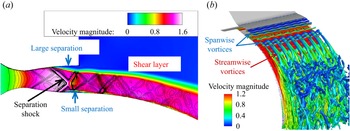
Figure 14(a) shows the shock wave structures near the jet exit, as well as their interactions with the boundary layer and shear layer. Due to the contrasting circumstances on both sides of the nozzle exit (free air on the outside and curved surface on the inside), the shock wave structure is asymmetric, causing the separation on the outside to be larger than that on the inside. Another effect of this forcing asymmetric is to stabilize the shock interaction here, which will be analysed later. Figure 14(b) shows the shear layer vortex structure using  $Q$-criteria; the spanwise vortices caused by K-H instability and the streamwise vortices caused by Taylor–Görtler-type instability can be observed. The spanwise vortices exhibit spanwise bending characteristics under the action of the streamwise vortices.
Typical ensemble-averaged flow structures, (a) shock waves in mid-span slice (colour contours: velocity magnitude, black lines: divergence of velocity), (b) vortex structures using  $Q$-criteria (
 $Q=100$, coloured by velocity magnitude).

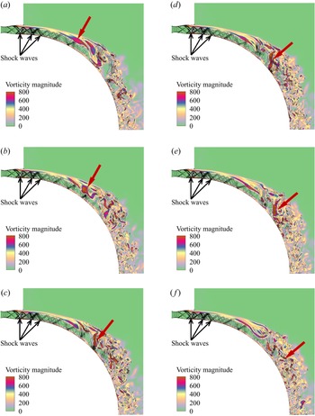
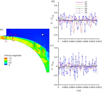
Johnson & Papamoschou (Reference Johnson and Papamoschou2010) have studied the unsteady shock behaviour in a simple over-expanded planar nozzle. Their experiments observed large-scale unsteadiness of the shock wave and found that the instability of the shock wave position led to enhanced mixing of the separated shear layer. When isolated from the unsteady shock motion, the alternating series of expansion and compression waves present downstream of the main separation shock likely has no significant impact on the stability of the downstream shear flow. Figure 15 shows the flow development of the mid-span plane at different times, the vorticity magnitude is shown in the colour contours, and the shock structures are shown through velocity divergence lines. Unsteady vortex shedding, transport and dissipation in the shear layer can be observed (indicated by red arrows), whereas no apparent unsteady motion is observed in the shock structure. Furthermore, the variation of velocity and density (non-dimensionalized by ambient air sound speed and density, respectively) near the shock wave and shear layer in the jet are monitored, and the time histories of these parameters are obtained (mean value is subtracted) (figure 16). Compared with the downstream  $P5$ and
 $P6$, the flow oscillation amplitude of
 $P1{-}P4$ near the jet exit is almost negligible. According to the study of Johnson & Papamoschou (Reference Johnson and Papamoschou2010), it could be concluded that the relatively steady shock structure has little impact on the instabilities of the downstream shear layer.
Instantaneous flow development in mid-span slice at different time steps (colour contours: vorticity magnitude, black lines: divergence of velocity); (a)  $0$, (b)
 $500t$ (
 $t$ is a time step), (c)
 $900t$, (d)
 $1100t$, (e)
 $1300t$ and ( f)
 $1500t$.

Time history of different monitoring points. (a) Schematic diagram of monitoring points, (b)  $U-U_{avg}$ and (c)
 $\rho - \rho _{avg}$.

According to the above analysis, streamwise vortices are observed, and they may play an important role in the jet shear layer instability. In this subsection, the generation and development of the streamwise vortices, and their role in the instability of the supersonic jet over a convex wall, will be clarified.
The mean vorticity transport equation provides a budget of the various effects contributing to a change in the mean vorticity. The mean vorticity equation is
 \begin{equation} \frac{{\partial \langle {\omega _j}\rangle }}{{\partial t}} + \langle {u_j}\rangle \frac{{\partial \langle {\omega _i}\rangle }}{{\partial {x_j}}} = \langle {\omega _j}\rangle \langle {s_{ij}}\rangle + \langle {{\omega' _j}} {{s'_{ij}}}\rangle - \frac{\partial \langle {{u' _j}}{{\omega'_{i}}}\rangle}{\partial x_j} + \nu \frac{{{\partial ^2}\langle {\omega _j}\rangle }}{{\partial {x_i}\partial {x_j}}}, \end{equation}
where the symbols  $\langle \rangle$ in the equation represent the ensemble average. It can be seen that the influences on the change of the mean vorticity include the mean term
 $\langle {\omega _j}\rangle \langle {s_{ij}}\rangle$, the turbulent term
 $\langle {{\omega ' _j}}{{s'_{ij}}}\rangle$, the turbulent diffusion term
 $- ({\partial \langle {{u' _j}}{{\omega '_{i}}}\rangle }/{\partial x_j})$ and the viscous dissipation term
 $\nu ({{{\partial ^2}\langle {\omega _j}\rangle }}/{{\partial {x_i}\partial {x_j}}})$.
Under a cylindrical coordinate system, consider the mean term of the streamwise vorticity component in the vorticity transport equation
 \begin{equation} {{\langle {\omega _j}\rangle \langle {s_{ij}}\rangle } |_\theta } = \langle {\omega _r}\rangle \frac{{\partial \langle {u_\theta }\rangle }}{{\partial r}} + \langle {\omega _\theta }\rangle \frac{{\partial \langle {u_\theta }\rangle }}{{r\partial \theta }} + \langle {\omega _z}\rangle \frac{{\partial \langle {u_\theta }\rangle }}{{\partial z}} - \frac{{\langle {u_\theta }\rangle \langle {\omega _r}\rangle }}{r}. \end{equation}
For a given streamwise location ( $\theta = \textrm {const.}$), the mean streamwise vorticity arising from the centrifugal effects in a mean term,
 $CFG(1) = ({1}/{r})({{\partial u_\theta ^2}}/{{\partial z}})$, is combined with the results of the skewness effect,
 $\langle {\omega _r}\rangle ({{\partial \langle {u_\theta }\rangle }}/{{\partial r}}) + \langle {\omega _z}\rangle ({{\partial \langle {u_\theta }\rangle }}/{{\partial z}})$ and the curvature effect,
 $- {{\langle {u_\theta }\rangle \langle {\omega _r}\rangle }}/{r}$. Similarly, the turbulent term,
 $CFG(2) = ({1}/{r})({{\partial {u'_\theta }^2}}/{{\partial z}})$, accounts for the mean vorticity arising from the turbulent stresses in the flow.
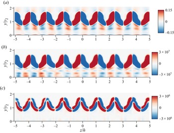
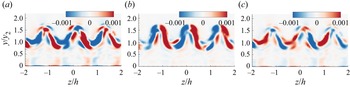
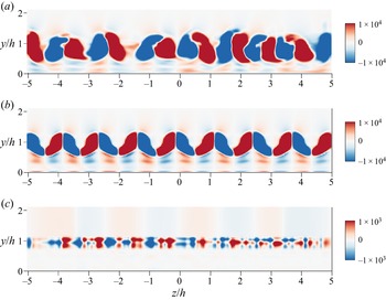
Pandey & Gregory (Reference Pandey and Gregory2020) used spanwise heterogeneities at the nozzle lip of a cylinder apparatus to force streamwise vortices in a low-speed incompressible jet over a convex wall. According to a similar analysis, they found that the centrifugal effect in the jet sustained the forced streamwise vortices. Figure 17 shows the normalized ensemble average of streamwise vorticity at  $\theta = 25^{\circ }$. The contours of the centrifugal effects in a mean term (figure 17b) show good correspondence with the ensemble-averaged vorticity contours (figure 17a), which suggests that the centrifugal effect dominants the streamwise vorticity production. For the centrifugal terms arising from the turbulent stresses (figure 17c), the contribution of this term has a pair of opposite vortices at the position of each streamwise vorticity cell, which would lead to the radial distribution of the streamwise vorticity shifting away from the wall. However, the contribution of this term is one order of magnitude smaller than that of the mean term. The conclusion is consistent with that of Pandey & Gregory (Reference Pandey and Gregory2020) in a low-speed incompressible jet over a convex wall.
Ensemble-averaged streamwise vorticity at  $\theta = 25^{\circ }$, (a) streamwise vorticity,
 $\omega _{\theta }\times y_2 / U_ {2Dmax}$, (b) streamwise vorticity due to centrifugal terms arising from the mean flow,
 $CFG(1)$, (c) streamwise vorticity due to centrifugal terms arising from the turbulent stresses,
 $CFG(2)$.

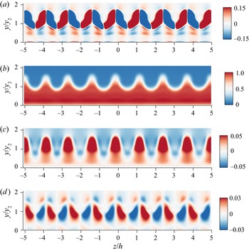
Figure 18 shows the ensemble-averaged contours of the streamwise vorticity and three velocity components in the spanwise plane. Under the action of the streamwise vortices, there are spanwise periodic upwash and downwash regions. The upwash action transports the high-speed flow from the inner layer to the outer part. The converse effect happens in the downwash regions. This transportation causes the spanwise inflection points of the velocity distribution (figure 18b–d) which will trigger the instability of the shear layer in the spanwise direction. In addition, the inflection point of the streamwise velocity distribution (figure 19) in the outer part of the jet triggers the roll-up of the spanwise vorticity tubes. The effects of upwash and downwash cause these inflection points to move outwards and inwards, respectively, resulting in the meandering of the spanwise vorticity tubes. Therefore, the streamwise vortices accelerate the instability of the shear layer by modulating the inflection instability of the spanwise flow.
Ensemble-averaged contours of the spanwise plane at  $\theta = 25^{\circ }$, (a) streamwise vorticity,
 $\omega _{\theta } \times y _2 / U_ {2Dmax}$, (b) streamwise velocity,
 $U/U_{2Dmax}$, (c) radial velocity,
 $V/U_{2Dmax}$, (d) spanwise velocity,
 $W/U_{2Dmax}$.

Streamwise velocity distribution at three spanwise locations ( $\theta = 25^{\circ }$).

The DMD analysis is performed on a consecutive sequence of 320 snapshots for the instantaneous streamwise vorticity fields at downstream location  $\theta = 25^{\circ }$. The time interval between two snapshots is
 $3.6 \times 10^{-6}$ s. The energies of the DMD modes as a function of frequency are shown in figure 20. The top four modes with the highest energy are marked in figure 20. Mode 1 and mode 2 are two steady modes, mode 3 and mode 4 are a pair of conjugate unsteady modes.
The DMD mode energy as the function of frequency.

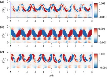
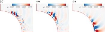
Figure 21 shows the spatial distribution of the modes marked in figure 20. The distributions of the steady mode1 (figure 21a) and mode 2 (figure 21b) are consistent with the turbulent stress contribution and mean flow contribution of the centrifugal effect in figure 17, respectively. This further confirms that the streamwise vorticity generated by the centrifugal effect in the jet is almost stable. The unsteady conjugate modes 3 and 4 (figure 21c) have an antisymmetric distribution at each pair of streamwise vortices. The time evolution of this mode is shown in figure 22, the spatial distribution changes little. However, the positive and negative values of this mode are just opposite from  $t_0$ (figure 22a) to
 $t_0+T/2$ (figure 22c). The effect of this mode is to cause the streamwise vortices to sway side to side, which is one of the ways to obtain energy from the mean flow and maintain instability.
Spatial distributions of the DMD modes; (a) steady mode 1, (b) steady mode 2 and (c) conjugate modes 3 and 4.

Time evolution of the conjugate modes 3 and 4; (a)  $t_0$, (b)
 $t_0+T/4$ and (c)
 $t_0+T/2$.

In the low-speed incompressible jet over a convex wall, a series of studies by Likhachev et al. (Reference Likhachev, Neuendorf and Wygnanski2001), Neuendorf et al. (Reference Neuendorf, Lourenco and Wygnanski2004) and Han et al. (Reference Han, de Zhou and Wygnanski2006) have indicated that streamwise vortices merge in the downstream direction to ensure the spanwise wavelength scales with the jet half-width. Pandey & Gregory (Reference Pandey and Gregory2020) have made similar observations in a forced convex wall jet. However, for the supersonic jet in this study, as shown in figure 23, the development of the streamwise vortices in the downstream direction is dominated by deformation, diffusion and breakage, rather than the merging of vortex pairs. This seems to be attributed to the influence of the compressibility effect since the roll-up and merging of vortices are suppressed by the strong compressibility effect in the planar mixing layer (Elliott et al. Reference Elliott, Mo and Arnette1995).
Ensemble-averaged streamwise vorticity from  $\theta = 25^{\circ }$ to
 $75^{\circ }$; (a)
 $25^{\circ }$, (b)
 $40^{\circ }$, (c)
 $55^{\circ }$ and (d)
 $75^{\circ }$.

Figure 24 shows the development of the flow velocity contours at various streamwise locations. Under the diffusion and transport of the streamwise vortices, the jet width increases, as does the spanwise bending of the shear layer. As the streamwise vortices are broken into smaller vortices, the jet transforms fully developed (self-similar region), and the flow in the spanwise direction tends to be uniformly distributed.
Ensemble-averaged streamwise velocity from  $\theta = 25^{\circ }$ to
 $75^{\circ }$; (a)
 $25^{\circ }$, (b)
 $40^{\circ }$, (c)
 $55^{\circ }$ and (d)
 $75^{\circ }$.

4.3. Turbulence in the supersonic convex wall jet
In the analysis of § 4.1, it has been found that, within streamwise location  $\theta = 30^{\circ }$, the jet half-width
 $y_2$ remains constant, while the shear layer vorticity thickness increases slowly. Then, the jet half-width
 $y_2$ increases linearly, and the vorticity thickness of the shear layer thickens exponentially. There is an inflection point in the vorticity thickness development near streamwise location
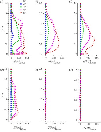
 $\theta = 60^{\circ }$. As shown in figure 25, the turbulent stress distributions further corroborate the analysis above. The stresses were averaged across the span to obtain the two-dimensional profiles. The jet half-width
 $y_2$ and the local span-averaged maximum streamwise velocity
 $U_{2Dmax}$ are used as the normalization of length scale and velocity scale, respectively.
Reynolds stress development from  $\theta = 5^{\circ }$ to
 $55^{\circ }$; (a)
 $\overline {{u}'^2}/U_{2Dmax}^2$, (b)
 $\overline {{v}'^2}/U_{2Dmax}^2$, (c)
 $\overline {{w}'^2}/U_{2Dmax}^2$, (d)
 $\overline {{u}'{v}'}/U_{2Dmax}^2$, (e)
 $\overline {{u}'{w}'}/U_{2Dmax}^2$ and ( f)
 $\overline {{v}'{w}'}/U_{2Dmax}^2$.

Turbulent stresses increase slowly within  $30^{\circ }$ since the shear layer is dominated by the large-scale spanwise vortices, and the instability in the flow has not been established. With the increasing importance of the streamwise vortices, the secondary instability caused by spanwise modulation triggers the instability of the shear layer, and turbulent stresses increase rapidly. In addition, the location of maximum stresses moves towards the wall (in the normalized sense) in the downstream direction (figure 25). This is presumably due to the radial diffusion of the streamwise vortices (figure 23). It should be noted that spanwise averaging of
 $\overline {{u}'{w}'}$ and
 $\overline {{v}'{w}'}$ over several wavelengths results in values close to zero.
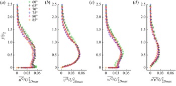
After  $\theta = 60^{\circ }$, with the further instability of the shear layer, the large-scale vortices are broken into small-scale vortices, and turbulence in the jet seems fully developed. Similar to the results of Neuendorf et al. (Reference Neuendorf, Lourenco and Wygnanski2004) and Pandey & Gregory (Reference Pandey and Gregory2020) in the low-speed jet, the streamwise velocity profiles of a convex wall supersonic jet are also self-similar when normalized by the jet half-width in radial coordinates and maximum jet velocity in velocity coordinates (figure 26). What is more, the normalized turbulence stresses in this region are self-similar as well (figure 27), which is not mentioned in previous studies.
Self-similar of streamwise velocity after  $\theta = 60^{\circ }$.

Self-similar of Reynolds stresses after  $\theta = 60^{\circ }$; (a)
 $\overline {{u}'^2}/U_{2Dmax}^2$, (b)
 $\overline {{v}'^2}/U_{2Dmax}^2$, (c)
 $\overline {{w}'^2}/U_{2Dmax}^2$ and (d)
 $\overline {{u}'{v}'}/U_{2Dmax}^2$.

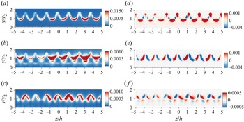
The spanwise distribution of the Reynolds stresses used in obtaining the spanwise-averaged profiles presented in figures 25 and 27 is shown in figure 28 at the downstream location  $\theta = 25^{\circ }$. The radial and spanwise axes have been normalized by jet half-width
 $y_2$ and nozzle slot height
 $h$, respectively. The local span-averaged maximum streamwise velocity
 $U_{2Dmax}$ is used as the normalization of the velocity scale. The Reynolds stresses are spanwise periodic, as expected from the periodicity caused by spanwise modulation of the streamwise vorticity in the mean flow (figure 18). There are spanwise periodic upwash and downwash regions under the action of the streamwise vortices. The streamwise and radial normal stresses are largest in the downwash regions, which is probably due to the relatively higher momentum close to the wall (figure 19). Conversely, the spanwise normal stresses are observed to be smallest in the downwash regions.
Reynolds normal stresses (a–c) and shear stresses (d–f) at  $\theta = 25^{\circ }$; (a)
 $\overline {{u}'^2}/U_{2Dmax}^2$, (b)
 $\overline {{v}'^2}/U_{2Dmax}^2$, (c)
 $\overline {{w}'^2}/U_{2Dmax}^2$, (d)
 $\overline {{u}'{v}'}/U_{2Dmax}^2$, (e)
 $\overline {{u}'{w}'}/U_{2Dmax}^2$ and ( f)
 $\overline {{v}'{w}'}/U_{2Dmax}^2$.

The streamwise vortices cause the spanwise periodic variation of the streamwise velocity (figure 18b), which leads to the change of the radial and spanwise gradient of the velocity. The radial gradient (figure 29a) has a negative maximum in the downwash region, which is associated with the largest negative spanwise vorticity. This determines that the streamwise–radial shear stress ( $\overline {{u}'{v}'}$) distributes as in figure 28(a). For the streamwise–spanwise (
 $\overline {{u}'{w}'}$) and radial–spanwise (
 $\overline {{v}'{w}'}$) shear stresses, they have a spanwise alternating positive and negative distributions, so the spanwise-averaged value is close to zero (figures 25e and 25f). The alternation regions of
 $\overline {{u}'{w}'}$ are associated with the spanwise shear seen in figure 29(b). While
 $\overline {{v}'{w}'}$ can be associated with the radial shear.
Contours of (a) radial gradient of streamwise velocity  ${\partial (U/U_{2Dmax})}/{\partial y}$, and (b) spanwise gradient of streamwise velocity
 ${\partial (U/U_{2Dmax})}/{\partial z}$.

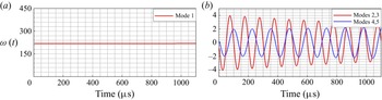
In order to investigate the typical modal characteristics in the streamwise direction, the DMD analysis is performed on the mid-span instantaneous density flow fields as well. The energies of the DMD modes as a function of frequency are shown in figure 30. In general, the modal energy decreases with the increase of frequency. This is expected because higher frequencies always seem to be associated with smaller-scale coherent structures. The top five modes with the highest energy and a pair of high-frequency conjugate modes are marked in figure 30. The time coefficient histories for these modes are presented in figure 31. Mode 1 is a steady mode, and the time coefficient is consistent with time. The rest are periodic modes with a negative growth rate.
The DMD mode energy as a function of frequency.

Time coefficients of the first five DMD modes.

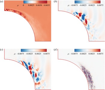
Figure 32 shows the spatial distributions of the DMD eigenmodes marked in figure 30. Mode 1 (figure 32a) is the steady mode, which represents the average information of the flow field. The time history of density (mean value is subtracted) at  $P5$ is shown in figure 16(a) and corresponding power spectrum shown in figure 34. The density oscillations there reflect vortex shedding in the shear layer. Power spectrum analysis shows a dominant frequency of
 $10\ 000$ Hz, which is consistent with the frequency of the conjugate modes 2 and 3 (
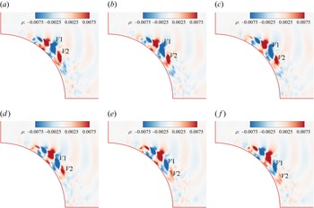
 $9989$ Hz) obtained from the DMD. This indicates that the conjugate modes 2 and 3 (figure 32b) are the vortex shedding modes, which represent the contribution of alternate vortex shedding in the shear layer to the flow development. Figure 33 shows the time evolution of the mode, in which the alternating density patterns represent large-scale vortical structures. A pair of negative and positive density fluctuations, which are marked
 $V1$ and
 $V2$, respectively, convect along with the shear layer. The positive density marked
 $V2$ begins to break at
 $t= t_0 + 4T/9$ in figure 33(e). The conjugate modes 4 and 5 (figure 32c) are the streamwise vortices’ action modes, which have a distribution extending from the shear layer to the inner part of the jet. The alternating lobes are tilted in the streamwise direction due to the inner part moving faster than the outer part. Pandey & Gregory (Reference Pandey and Gregory2020) observed similar tilted lobes associated with a secondary instability of the streamwise vortices in the incompressible jet over a convex wall (see figure 23 of Pandey & Gregory Reference Pandey and Gregory2020). In addition, some prominent features can be seen in figure 32. The unsteady modes with the highest energy are distributed from
 $\theta = 30^{\circ }$ to
 $\theta = 60^{\circ }$ in the streamwise direction, which corresponds to the region of the rapid growth of turbulent stresses (figure 25). The high-frequency mode associated with smaller-scale coherent structures is distributed in the rear of the jet, where turbulence is fully developed and self-similar (figures 26 and 27).
Spatial distributions of the density DMD modes; (a) steady mode 1, (b) conjugate modes 2 and 3, (c) conjugate modes 4 and 5 and (d) conjugate modes 292 and 293.

Time evolution of conjugate modes 2 and 3; (a)  $t_0$, (b)
 $t_0+T/9$, (c)
 $t_0+2T/9$, (d)
 $t_0+3T/9$, (e)
 $t_0+4T/9$ and ( f)
 $t_0+5T/9$.

4.4. Influence of compressibility effect
Different exit velocities and densities can be produced for a fixed convergent–divergent nozzle geometry by keeping the inlet pressure ratio constant and varying the temperature ratio. Adjusting the pressure ratio can result in varied outlet Mach numbers. This subsection will investigate the impact of these two factors on the development of supersonic jet flow over a convex surface in order to evaluate the compressibility effect.
In the compressible planar jet, the convective Mach number ( $M_c$) is an effective parameter to quantify the level of compressibility in the mixing layer. It is defined as
 ${M_c} = ({{{U_1} - {U_2}}})/({{{a_1} + {a_2}}})$, for two gases with the same specific heat ratio (Bogdanoff Reference Bogdanoff1983; Papamoschou & Roshko Reference Papamoschou and Roshko1988). However, due to the influence and constraint of the wall, the situation for a compressible jet over a convex wall jet in this study becomes considerably more complex. Because of the viscosity and entrainment effect, the flow velocity on both sides of the shear layer is no longer uniform. Therefore,
 $M_c$ is assessed using the nozzle exit flow characteristics in this study.
4.4.1. Temperature ratio effect
At a fixed  $NPR=3.0$, numerical simulations are performed for three distinct temperature ratios
 $T_0/T_{amb}=1.2$,
 $1.6$ and
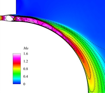
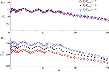
 $2.0$. As shown in figure 35, the jet Mach number contours of different temperature ratios are substantially the same. This is further corroborated by the maximum Mach number along the streamwise direction shown in figure 36(a). Figure 36(b) demonstrates that, when the temperature ratio increases, the jet velocity increases owing to the change in sound speed associated with the temperature change.
Density time history of  $P5$ in figure 16 (a)
 $\rho - \rho _{avg}$ and (b) corresponding power spectrum,
 $PSD$.

Mean flow Mach contours of different temperature ratios ( $T_0/T_{amb}=1.2$: colour contours,
 $T_0/T_{amb}=1.6$: solid lines,
 $T_0/T_{amb}=2.0$: dashed lines).

Ensemble- and spanwise-averaged (a) maximum Mach number, and (b) maximum velocity along the streamwise direction.

Considering the convective Mach number calculation formula  ${M_c} = ({{{U_1} - {U_2}}})/({a_1} + {a_2}) = {{M{a_1}}}/({{1 + {a_2}/{a_1}}})$, where
 $U_2=0$. The variation of
 $M_c$ is dominated by the jet Mach number and the speed of sound. However, the jet density decreases as the temperature ratio increases (figure 37), and the change in density can be reflected in the change in the local speed of sound. The convective Mach numbers of the three temperature ratios are 0.64, 0.69 and 0.73. The specific parameters are shown in table 1, considering the flow non-uniformity at the nozzle exit, the Mach number, velocity and corresponding convective Mach number are characterized using the maximum values at the nozzle exit.
Mean flow density contours for different temperature ratios; (a)  $NPR=3.0, T_0/T_{amb}=1.2$, (b)
 $NPR=3.0, T_0/T_{amb}=1.6$ and (c)
 $NPR=3.0, T_0/T_{amb}=2.0$.

Detailed parameters for different temperature ratios.

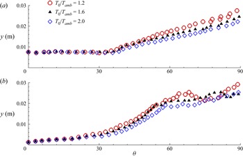
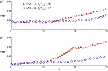
Figure 38 shows the development of the jet half-width and vorticity thickness of the shear layer along the streamwise direction. The three states have the same change trend, and the positions of the jet rapid growth and the self-similar region are nearly identical. This implies that the velocity difference caused by changes in the temperature ratio has little effect on jet development. However, increasing the temperature ratio causes a slight increase in the convective Mach number (from 0.64 to 0.73, table 1), which may be responsible for some suppression of the jet half-width and shear layer vorticity thickness in figure 38.
Ensemble- and spanwise-averaged (a) jet half-width, and (b) vorticity thickness of the shear layer along the streamwise direction.

4.4.2. Pressure ratio effect
Through the above analysis, it is known that the velocity increase induced by the temperature ratio increase has little effect on the development of the jet shear layer, and the change of  $M_c$ is dominated by the Mach number. Here, the influence of the compressibility effect on the jet over a convex wall is studied by changing the inlet pressure ratio to control the Mach number at the nozzle exit.
Three different inlet pressure ratios of 2.0, 3.0 and 3.9 ( $T_0/T_{amb}=1.2$) are adopted to study the compressibility effect. Figure 39 shows the Mach contours of these three pressure ratios; with the increase of pressure ratio, the jet over-expansion characteristics are gradually improved, and the shock wave structure in the nozzle is pushed outward. Figure 40 shows the Mach number distributions near the nozzle exit; it can be seen that the Mach number at the outlet gradually increases, as does the jet width. Table 2 shows the detailed parameters of three different pressure ratio states. The numerical nozzle exit Mach numbers are 1.04, 1.33 and 1.93, and the corresponding convective Mach numbers are 0.52, 0.66 and 0.88, respectively. The first two states are moderately compressible conditions, and the last one is a highly compressible condition according to the compression definition in the planar jet (Zhang et al. Reference Zhang, Tan and Li2017).
Mean flow Mach contours of different pressure ratios; (a)  $NPR=2.0$, (b)
 $NPR=3.0$ and (c)
 $NPR=3.9$.

Mach profiles at nozzle exit.

Detailed parameters for different pressure ratios.

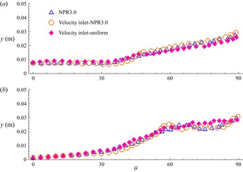
There are different separation zones in the nozzle with varied inlet pressure ratios (figure 39), and the nozzle exit flows are non-uniform as well (figure 40). These factors could have impacts on the instability of the shear layer. Firstly, to eliminate the effects of flow structures within the nozzle (shock waves and separation zones), the nozzle is replaced by a velocity inlet boundary condition, where the flow is given as the mean flow at the nozzle outlet of  $NPR=3.0$. The schematics of these two configurations are shown in figures 41(a) and 41(b). Secondly, to assess the effect of non-uniform flow, another uniform velocity profile of
 $Ma=1.33$ is provided at the velocity inlet. The non-uniform/uniform Mach profiles at the velocity inlet are depicted in figure 41(c).
Schematics of pressure inlet with nozzle and velocity inlet without nozzle, and non-uniform/uniform Mach profiles at velocity inlet. (a) Pressure inlet, (b) velocity inlet and (c) Mach profiles at velocity inlet.

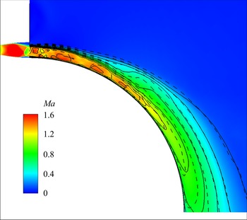
Figure 42 shows the Mach contours/lines of different boundary conditions in figure 41. The similar Mach distributions in figure 42 indicate that they have nearly identical jet development. Further, to quantitatively compare the development of the jet, figure 43 presents the development of the jet half-width and the shear layer vorticity thickness along the streamwise direction. As there are few differences between them, the instability of the shear layer is nearly not influenced by the flow structures within the nozzle, such as shock waves and separation zones, or by the non-uniform flow at the nozzle exit. This finding further supports the conclusion that the steady shock structures in the jet have limited impact on the shear layer instabilities, as discussed in § 4.2.
Mean flow Mach contours of different temperature ratios (colour contours:  $NPR=3.0$ with nozzle, solid lines: velocity inlet using the mean flow of
 $NPR=3.0$ with nozzle, dashed lines: uniform velocity inlet).

Ensemble- and spanwise-averaged (a) jet half-width, and (b) vorticity thickness of the shear layer along the streamwise direction.

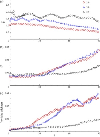
The streamwise direction development of the maximum Mach numbers, the jet half-widths and the vorticity thicknesses are shown in figure 44. The Mach number increases with the increase of the pressure ratio, in other words, the compression effect is enhanced. The jet half-width (figure 44b) and vorticity thickness (figure 44c) development of the two moderately compressible conditions have similar variations. However, as the pressure ratio increases from 2.0 to 3.0, the streamwise location where rapid growth of the jet half-width and vorticity thickness is still delayed from  $\theta = 20^{\circ }$ to
 $30^{\circ }$ due to relatively stronger compressibility. For the highly compressible condition, the development of the jet half-width and vorticity thickness is strongly restrained.
Ensemble- and spanwise-averaged (a) maximum Mach number, (b) jet half-width and (c) vorticity thickness of the shear layer along the streamwise direction.

Furthermore, when the outlet flow characteristics of case 3 in table 1 and table 2 are compared, the outlet velocities of the two cases are nearly identical. The distinction is due to the differing Mach numbers induced by the different pressure ratios. For these two conditions, figure 45 shows the development of the jet half-width and shear layer vorticity thickness along the streamwise direction. It could be deduced that the increase in Mach number has a greater influence on the growth of the shear layer than the change in velocity.
Ensemble- and spanwise-averaged (a) jet half-width, and (b) vorticity thickness of the shear layer along the streamwise direction.

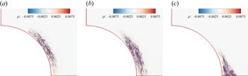
According to the analysis in § 4.3, the highest energy unsteady mode and the high-frequency mode are associated with the rapid growth region and the self-similar region of turbulent stresses, respectively. Figures 46 and 47 show the spatial distributions of the highest energy unsteady modes and the high-frequency modes. It can be seen that, with the increase of the pressure ratio, that is, when the compressibility effect increases, the growth region moves downstream, and the distribution range increases. This means that the stronger compressibility effect makes the shear layer instability occur later and the instability speed be lower (figure 46). Correspondingly, the self-similar region is also delayed downstream (figure 47).
Spatial distributions of the highest energy unsteady density DMD modes; (a)  $NPR=2.0, M_c = 0.52$, (b)
 $NPR=3.0, M_c = 0.64$ and (c)
 $NPR=3.9, M_c = 0.88$.

Spatial distributions of the high-frequency DMD modes (mode 292); (a)  $NPR=2.0, M_c = 0.52$, (b)
 $NPR=3.0, M_c = 0.64$ and (c)
 $NPR=3.9, M_c = 0.88$.

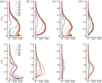
The development of Reynold stresses for the moderately compressible condition  ${PR=3.0}$ has been discussed in § 4.3 (figures 25 and 27). It was indicated that the normalized turbulence stresses show self-similar after downstream location
 $\theta = 60^{\circ }$. Figure 48 shows the development of Reynolds stresses at another moderately compressible condition
 $NPR=2.0$ and a highly compressible condition
 $NPR=3.9$. For the state of
 $NPR=2.0$, the normalized turbulence stresses become self-similar earlier at
 $\theta = 50^{\circ }$. While for the highly compressible state, the streamwise normal stress (
 $\overline {{u}'^2}$) and streamwise–radial shear stress (
 $\overline {{u}'{v}'}$) seem to show weak self-similarity after
 $\theta = 75^{\circ }$, the radial normal stress (
 $\overline {{v}'^2}$) and spanwise normal stress (
 $\overline {{w}'^2}$) do not show obvious self-similarity.
The development of Reynolds stresses, top:  $NPR=2.0, M_c =0.52$, bottom:
 $NPR=3.9, M_c =0.88$ showing (a)
 $\overline {{u}'^2}/U_{2Dmax}^2$, (b)
 $\overline {{v}'^2}/U_{2Dmax}^2$, (c)
 $\overline {{w}'^2}/U_{2Dmax}^2$ and (d)
 $\overline {{u}'{v}'}/U_{2Dmax}^2$.

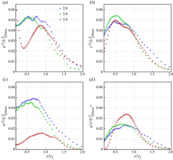
Figure 49 plots similarity profiles for the two moderately compressible conditions at  $\theta = 75^{\circ }$ and the highly compressible condition at
 $\theta = 85^{\circ }$. The peak values of streamwise normal stress (
 $\overline {{u}'^2}$) and radial normal stress (
 $\overline {{v}'^2}$) show little change with
 $M_c$, while the spanwise normal stress (
 $\overline {{w}'^2}$) profile peak values clearly decrease with
 $M_c$ increasing. This indicates that the compression effect has a strong inhibitory effect on spanwise fluctuations.
Reynold stresses similarity profiles for all three  $M_c$ cases; (a)
 $\overline {{u}'^2}/U_{2Dmax}^2$, (b)
 $\overline {{v}'^2}/U_{2Dmax}^2$, (c)
 $\overline {{w}'^2}/U_{2Dmax}^2$ and (d)
 $\overline {{u}'{v}'}/U_{2Dmax}^2$.

According to the analysis in §§ 4.2 and 4.3, it has been found that streamwise vortices play an important role in spanwise modulation and shear layer instability. The streamwise vorticity contours at downstream location  $\theta = 25^{\circ }$ for all three
 $M_c$ cases are shown in figure 50. The highly compressible condition significantly inhibits the generation of large-scale streamwise vortices. This inhibition weakens the ability of spanwise modulation and secondary instability in the shear layer.
Ensemble-averaged streamwise vorticity contours at  $\theta = 25^{\circ }$; (a)
 $NPR=2.0, M_c = 0.52$, (b)
 $NPR=3.0, M_c = 0.64$ and (c)
 $NPR=3.9, M_c = 0.88$.

5. Conclusions
In the present study, numerical investigation of the supersonic jet over a convex wall was carried out with the DDES method based on the SST turbulence model. In particular, the centrifugal effect and its role in instability, development of the turbulence stresses and the influence of the compressibility effect were investigated. The main conclusions of this study are summarized as follows.
The streamwise vortices are observed in the shear layer, and the analysis of the streamwise vorticity transport equation reveals the generation mechanism of the streamwise vortices. The mean term of the centrifugal effect dominates the generation of the streamwise vortices, whereas the turbulent fluctuation term influences their radial distributions. Like the incompressible convex wall jet, the streamwise vortices also play an important role in the shear layer instability in the compressible convex wall jet. The spanwise modulation of the streamwise vortices produces the secondary instability of the shear layer, which leads to the rapid growth of the shear layer. The secondary instability is maintained through a side-to-side swaying motion to obtain energy from the mean flow according to the DMD analysis of the streamwise vorticity fields in the spanwise section.
In terms of the turbulence characteristics, the spanwise periodic upwash and downwash regions under the action of the streamwise vortices make the Reynolds stresses exhibit spanwise periodic distributions. The streamwise development of the supersonic convex wall jet can be divided into the growth region and the self-similar region. In the growth region, the rapid increase of turbulence stresses can be attributed to the shear layer instability induced by streamwise vortices. In the self-similar region, in addition to the velocity profiles, the normalized turbulent stresses have good self-similar properties as well. The DMD analysis of the mid-span section indicates that the growth region is dominated by low-frequency large-scale vortex structures, while the self-similar region is associated with the high-frequency small-scale structures.
The convective Mach number ( $M_c$) is an effective parameter to quantify the level of compressibility in a convex wall jet. Compared with the jet velocity change, the change of Mach number has a more significant impact on
 $M_c$, as well as on the shear layer development. The compressibility effect significantly inhibits the generation of large-scale streamwise vortices and the growth of the shear layer in the supersonic convex wall jet. Additionally, the peak values of spanwise normal turbulent stress profiles in the self-similar zone obviously decline as the convective Mach number increases, although peak values of other turbulent stresses vary little. It implies that the compressibility effect enhances turbulence anisotropy.
Declaration of interests
The authors report no conflict of interest.
Funding
This study was co-supported by the National Natural Science Foundation of China (No. 11972308 and No. 11902265) and the National Major Basic Research Project 1912.
Data availability statement
The data that support the findings of this study are available from the corresponding author upon reasonable request.