

Social scientists have so far not given much systematic attention to modelling the dynamics of resource expenditure in a competition between political parties, or candidates, when these are thought of as full time image-selling agencies. Most studies of campaign expenditure ignore temporal data, and standard texts generally do not mention time. This article is part of a more general study that attempts to fill some of this gap.
The main question considered in the study is, what can formal theory tell us about the way in which competing parties or candidates spend their resources over time?Footnote 1 To save repetition, I will refer only to parties in what follows. Some casual observation and inference from works like those of Fisher and of Whitely and Seyd seem to show that expenditure tends to increase as the election approaches.Footnote 2 Although this pattern might seem too obvious to warrant consideration, it is only one possible trajectory and requires explanation. Is there any reason why expenditure should increase over the electoral period? Why not spend all the resources at the beginning, or at the end? It might be assumed, on the one hand, that voters are myopic and have short memory spans, as in the ‘what have you done for me lately?’ school of explanation.Footnote 3 On the other hand, it might also be assumed that voters value consistency and trust, and that support is built up over the long run.Footnote 4 It is not at all clear which of these assumptions is to be preferred, or even whether assumptions about voters’ attention spans give anything like a complete explanation. What if voters did not forget, or did not value consistency? What if there are factors, inherent in the process of competition itself, that are neither obvious nor accessible to direct observation?
The specific purpose of the study is to examine a stripped-down model of the dynamics of campaign expenditure, in which voters neither value long-term consistency nor forget over time, in order to answer some of these questions. This is done for a competition between two parties under a number of different information conditions. I compare these results with the case where there is only a single party.
This article presents the results of the study for a closed-loop competition where parties continually adjust their expenditure as they get information about their level of support from opinion polls and other sources.Footnote 5
The main results are that, despite the fact that voters do not forget, both parties increase their rate of resource expenditure on marketing through the entire period between elections. In addition, the opposition spends more than the government in every time interval if the government has higher initial levels of support. In contrast, where there is only a single party trying to increase its support, it spends at a constant rate.
An interesting illustration of the way in which competition influences the dynamics of expenditure is provided by the idea that when parties start out with equal support, they have to constantly increase their spending in order to retain their initial position. This is often known as the ‘Red Queen effect’.Footnote 6
I set out the paper as follows. In the next section, the model is specified. This is analysed in the following section for one party. It is analysed for competition between two parties in the subsequent section.
The Model And Discussion Of The Problem
The Basic Model
The model is constructed by assuming that there is a government and an opposition and that each party wants to maximize its support at an election held at some fixed time in the future by spending an all-purpose resource on marketing over the period between elections. The assumption that there is no discontinuity at the election captures the idea that parties are forward looking and that the level of support matters. The resource includes money spent on advertising and the time and effort that candidates, volunteers and party members spend on things like appearances at public functions, selling policies and attending cake stalls and talk-back shows. It is assumed, for simplicity, that different types of resource can be expressed on a common scale. Although there is a cost attached to spending resources, there is no limit on the amount that can be spent because it seems reasonable to assume that parties can run up debts in money and goodwill.Footnote 7 It is assumed that each individual in the population supports one of these parties. In order to make the analysis tractable, it is assumed that the policies of the parties are fixed at the beginning of each electoral cycle.
It is also assumed that support increases at a declining rate with the amount of resources a party spends, everything else being constant. It might be imagined, for example, that each party has a natural constituency and that the closer a voter is to this constituency, the more easily it is won over by the efforts of that party. As a voter gets further away, more effort is required to gain support.Footnote 8
The dynamics of this competition are analysed as a differential game in continuous time with a closed-loop state feedback information structure with no memory. This means that parties get reports on their level of support at each instant, and continually adjust their expenditure to the optimum level. In this way, the results of the strategies of both parties are constantly fed back to the decision-making process. This assumption also highlights the important point that it is not the action of the opponent that matters, but its effect on the level of support.
Other information structures, such as open-loop information, where parties commit expenditure at the beginning of the game, and Stackelberg information, where one party moves first, are also important to get a complete picture of the dynamics of competition, but they are not considered here.Footnote 9
In order to give some intuition to those unfamiliar with this type of differential game, I give a simple example, and some explanation, in the section dealing with one party only, for the case where there is only one party and two time periods. It will do no harm to think of the continuous time game as a generalization of the ideas behind this example.Footnote 10
The Formal Set-Up
The government and the opposition are referred to as Party 1 and Party 2 and denoted by the subscripts 1 and 2, respectively. Time is denoted by t. The resource expenditure of the government at time t is u 1(t) and that of the opposition is u 2(t), and the cost of expenditure is f 1(u 1) and f 2(u 2). The fraction of the population that makes up the natural constituency of party i is written qi and, for simplicity, set as q 1 = q 2 = q. Without loss of generality, change coordinates to set q = 0. The fraction of the population that supports the government is x(t). This means that support for the opposition is 1 − x(t).
The effect of spending by the government and opposition on the rate of change in support is written as:

where  Reference to time is suppressed to simplify the notation.Footnote 11
For tractability, the cost functions, fi, are simplified and it is assumed that the parties attempt to maximize payoff functions of the form

for i = 1, 2 subject to the dynamics in Equation 1. ci > 0 is a parameter that captures any differences in the cost to each party of spending resources and may depend on such things as the level of donations, availability of voluntary labour and so on.
Even though a winning majority is greater than half, the analysis also covers cases where the initial level of support for the government takes a value  . Party support, as opposed to actual votes, could be less than half, or tied, for any number of reasons. Maybe a supporter of the opposition forgot to vote, or submitted a spoiled ballot, for example.
Before analysing two-party competition, I consider the trajectory of expenditure for the case where there is a single party, for the purpose of providing a point of comparison.
Optimal Expenditure Without Competition
The most important result for the case where only a single party is trying to buy support is that the optimal programme is to spend resources at a constant rate throughout the entire period. This is an interesting result. It tells us that any deviation from this can be attributed to the effects of competition. Before analysing the general case, I provide the promised example.
The Two-Step Case as an Example
The model is simplified for the purposes of this example by setting c = 1 and k = 1, and the more general case is dealt with below. Since there is only one party, subscripts and superscripts can be dropped to clean up the notation. This allows us to rewrite Equations 1 and 2 for the two-step problem as

and

In order to capture the idea that parties are updating their expenditure at time t given the level of support at the beginning of the period, write v(t) as the optimum payoff from time t forward. This means that, beginning at the last period where a move is possible, the optimum payoff is

which can be achieved by substituting for x(2) and maximizing with respect to u(1) to get

It can be seen from this that the choice of u at time t = 1 depends on the support level at that time. Putting this back into the original expression and simplifying gives

We now go back to the first period at t = 0 where the optimum payoff will be

and substituting for x(1) gives v(0) in terms of u(0) and x(0). Maximizing this for u(0) and rearranging gives

and again taking the first order conditions gives

It is now possible to rewrite x(1) in terms of x(0) in the equation for u(1). A little manipulation gives

and expenditure is constant.
The Continuous Time Case
The dynamics for the continuous time model are now solved by generalizing these ideas to an arbitrarily large number of moves. This is done for the more general case where c > 0 and k > 0. We have

and the payoff function is given by J 1 in Equation 2. In order to generalize the idea of backward induction, it is necessary to use the Hamilton–Jacobi–Bellman equation from optimal programming. Write the value of the game from time t and initial condition x 0 as ω(t,x 0) and the partial derivative of ω with respect to any variable z as  . This gives us the partial differential equation

In order to get some more information on this, maximize the term in the brackets with respect to u to get

In most cases, it would be difficult to get an analytical solution for the partial differential equation we get from substituting this back onto the equation for ωt. In this case, we can use the Pontryagin principle to show that

for r some constant. This means

where  and expenditure is constant as in the two-step case.
It is worthwhile noting that this result is not limited to the specific assumptions made about the dynamics of support. It can be generalized to any specification of the dynamics of the form

Two-Party Competition
The general result for the case where parties are competing for support is that the optimal programme for each party is to increase its expenditure for the entire time period. This gives an immediate, and important, difference between the dynamics of two-party competition and the optimal programme for a single party. It is also shown that, when k 1 = k 2 = k, and the government has more initial support, the opposition always spends more than the government does. When the government and the opposition have the same initial support, we get the Red Queen effect. It has been necessary to restrict the analysis to the case where there is some symmetry and  for i = 1, 2, for c ≥ ε where ε is not arbitrarily small. The ratio
 is an important parameter for all the differential games of party competition I have analysed in the work referred to above.Footnote 12 It can be thought of, roughly, as telling us something about the relative impact of spending on marketing per unit of cost.Footnote 13
In order to get a solution, the Hamilton–Jacobi–Bellman equation is used in the same manner as before with superscripts to denote the players. This gives

with the analogous expression for  .
It is possible to solve Equation 3 in terms of a new function of time ϕ(t), which has a similar place in the equations for the trajectories as the costate in the Pontryagin theorem.Footnote 14 Differentiating this with respect to time gives

and this can be used to get

In order to get the trajectory of expenditure, differentiate the expression for ui with respect to time in these equations. By substituting from Equation 1 and for ϕ into the result and doing a little work, we get

for c which is not arbitrarily small. This means ui is increasing for all t for i = 1, 2.
Substituting the expressions for u into Equation 1 and simplifying gives the trajectory of support for the government along the optimal path as

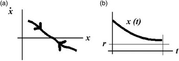
and it follows immediately that the system has an equilibrium at  . See Figure 1a.
The dynamics of support for the government part:  .

In order to get more detail on the dynamics, consider what happens when the initial level of support is varied. The following cases are of interest.
Case (i). The government has more initial support than the opposition and  . It follows directly from Equation 5 that

and support for the government falls for the entire period. In addition, it can be shown that  to give the trajectory in Figure 1b. It is immediate from Equation 5, or from the sign on
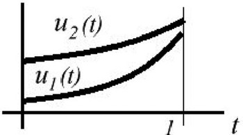
 , that the opposition party tries harder and spends more than the government does for the entire period. It is also possible to use the trajectory for x together with Equation 5 to get

for all t∈[0,1]. See Figure 2 for an example.
Example of trajectories of resource expenditure

In the converse case where  , it is easy to see that the government spends more than the opposition does for the entire period and its support increases.
Case (ii). Each party is supported by half the population at the beginning of the time period. It is immediate from Equation 7 that

which means – from Equation 6 – that each party is increasing its expenditure in order to stand still.
Conclusion
This article attempts to make up some of the gap in our theories of the dynamics of competition between political parties for support. It shows that, even when voters are not myopic, both parties increase their spending over time. Contrasting these results with spending by a single party shows that this increase results from the nature of the competition itself.
 term.