1 Introduction
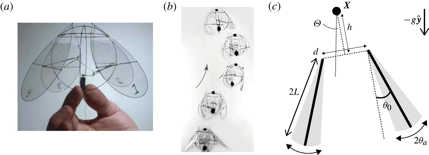
In the effort to design micro aerial vehicles (MAVs), biologically inspired flapping-wing ornithopters, as an alternative to helicopters, have shown great potential in achieving manoeuvrability and stability (Gerdes, Gupta & Wilkerson Reference Gerdes, Gupta and Wilkerson2012; Lentink Reference Lentink2013). Recently, a manoeuvrable and stable flapping-wing machine, using a stroke reminiscent of the swimming motions of a jellyfish, was fabricated at the NYU Applied Math Lab by Ristroph & Childress (Reference Ristroph and Childress2014). This ‘flying jellyfish’ consists of four lightweight flapping wings that are driven inward and outward reciprocally by a motor (figure 1
a,b). The total mass of the machine is 2.1 g, with the 1.1 g motor taking up more than
 $50\,\%$
of the total mass. Three manoeuvring flying modes were presented in their work – hovering, ascent and forward flight. Different manoeuvring modes were achieved through adjusting the motor voltage and linkage lengths, which changed the flapping frequency and the flapping amplitude, respectively. Of the two prototype machines, having the motor located either at the top and the bottom, respectively, only the bottom-heavy flyer showed stability in the upright orientation. This flyer recovered from large tilts by relying only on the aerodynamics of its flapping wings, and its self-righting hovering flight can last for hundreds of wing beats. This intrinsic aerodynamic stability has distinguished the jellyfish-like ornithopter from other state-of-the-art miniature ornithopter designs aiming to imitate the flapping motion of actual flyers in nature, such as flies, bees and hummingbirds (e.g. van Breugel, Regan & Lipson Reference van Breugel, Regan and Lipson2008; Ma et al.
Reference Ma, Chirarattananon, Fuller and Wood2013). Such flapping motions have been shown to be aerodynamically unstable in the last decade by controlled experiments, aerodynamic models and computational fluid simulations (Sun & Xiong Reference Sun and Xiong2005; Faruque & Humbert Reference Faruque and Humbert2010; Ristroph et al.
Reference Ristroph, Ristroph, Morozova, Bergou, Chang, Guckenheimer, Wang and Cohen2013). Both natural flyers and bio-mimetic aerial robots require additional stabilizing mechanisms, for instance feedback controllers and stabilizing surfaces, to maintain an upright orientation during flight. As even smaller robots are built, it will become even more challenging to implement these control and stability schemes. For this reason, the rather simple jellyfish-like flyer shows promise in yielding a manoeuvrable and stable MAV.
(a) The jellyfish-like flying robot fabricated by Ristroph & Childress (Reference Ristroph and Childress2014). A motor pulls in and pushes out four lightweight flapping wings. (b) Free stable ascent of the bottom-heavy prototype machine recorded by a high-speed camera, showing snapshots every four wing beats. (c) Two-dimensional mathematical model. Two rigid plates, each of length
 $2L$
, are driven to flap with prescribed mirror-symmetric sinusoidal pitching motions of amplitude
 $\unicode[STIX]{x1D703}_{a}$
. The wings’ base opening angle is
 $\unicode[STIX]{x1D703}_{0}$
. The hinges of the two wings are separated by a distance
 $d$
. The distance from the centre of mass
 $\boldsymbol{X}$
to the wing hinges is denoted by
 $h$
(centre-of-mass location).
 $\unicode[STIX]{x1D6E9}$
is the flyer’s tilt angle to the vertical direction. Panels (a) and (b) courtesy of Ristroph & Childress (Reference Ristroph and Childress2014).

The flying motion of the jellyfish-like machine resembles the shape changes of jet-propelled aquatic creatures such as the jellyfish, squid and octopus. To obtain locomotion, the jellyfish contracts and expands its bell to accelerate the fluid within the body. The vortex shedding and vortex ring formation during this process have been visualized and analysed by Dabiri et al. (Reference Dabiri, Colin, Costello and Gharib2005). Some recent experimental and theoretical studies have focused on jellyfish kinematics and performance (McHenry & Jed Reference McHenry and Jed2003; Peng & Alben Reference Peng and Alben2012), and a common interest between experimentalists and theorists is to seek an efficient contraction–expansion movement of jellyfish propulsion (Dabiri, Colin & Costello Reference Dabiri, Colin and Costello2006; Alben, Miller & Peng Reference Alben, Miller and Peng2013; Hoover & Miller Reference Hoover and Miller2015). The first attempt to implement an opening–closing motion in an aerial flyer design appeared in Childress, Vandenberghe & Zhang (Reference Childress, Vandenberghe and Zhang2006), where a flexible lightweight flapper opens and closes its body passively in a vertically oscillating background airflow. Hovering flight of the flapper was found, with its lift generation due to the vortex shedding of a shape-changing body (Spagnolie & Shelley Reference Spagnolie and Shelley2009). In subsequent efforts of Liu et al. (Reference Liu, Ristroph, Weathers, Childress and Zhang2012) and Weathers et al. (Reference Weathers, Folie, Liu, Childress and Zhang2010), a rigid hollow pyramid-shaped flyer was also found able to hover passively in an oscillating background flow, and displayed an intrinsic hovering stability depending on the centre-of-mass location. Huang, Nitsche & Kanso (Reference Huang, Nitsche and Kanso2015) studied this hovering dynamics numerically, mapping out regions of stability and instability, using a vortex sheet model for body and wake. In a subsequent study, again using a vortex sheet model, Huang, Nitsche & Kanso (Reference Huang, Nitsche and Kanso2016) studied the effects of varying the background flow and pyramid shape on the dynamics.
The Reynolds number of these passive aerial flyers, as well as the active aerial jellyfish-like machine, is
 $Re\sim 10^{4}{-}10^{5}$
. High Reynolds number fluid flows are often associated with unsteady and complex vortex dynamics, which makes the study of aerial flyers challenging. Moreover, for aquatic jellyfish their body density is nearly identical to that of water (Lucas et al.
Reference Lucas, Pitt, Purcell, Lebrato and Condon2011), so weight support and upright stability are not important hydrodynamic issues. This is not so for an aerial flyer, and for the air jellyfish, maintaining an upright orientation throughout the flight becomes a distinct design issue.
The main point of this paper is to use computational simulations to examine the aerodynamics and stability of a simplified jellyfish-like flying machine. We consider a two-dimensional (2-D) mathematical model (figure 1 c) comprised of two massless flapping wings with prescribed mirror-symmetric pitching motions, and a volumeless centre-of-mass body that mimics the motor mass of the actual device by Ristroph & Childress (Reference Ristroph and Childress2014). While we examine the flows and dynamics in the context of an idealized model of a specific device, jet-based locomotion is quite common in nature, e.g. jellyfish, scallops and squid. As far as we know, there is no theoretical work on stability of this locomotion, which is a concern for any body that is more dense than the fluid, for example, hard-shelled scallops (Shumway & Parsons Reference Shumway and Parsons2011).
For high Reynolds number flows, the computational method is challenging due to the complex vortex wake dynamics (Saffman Reference Saffman1993). For accuracy, most methods for fluid–structure interaction problems, such as the immersed boundary method (Peskin Reference Peskin2002), demand a fine computational grid near the object boundary so as to resolve the thin boundary layers, as well as fine grids to resolve the nearly singular vorticity field. In our study, we instead use an inviscid 2-D vortex sheet model which captures the vorticity distribution along the body and the free vortex dynamics, as well as the unsteady vorticity shedding from the wing tips. This boundary integral model is numerically solved through a regularized vortex sheet method. The method was first developed for the dynamics of a free vortex sheet (Krasny Reference Krasny1986), and was later widely applied to fluid–structure interaction problems at high
 $Re$
, such as flow exiting a tube (Nitsche & Krasny Reference Nitsche and Krasny1994), falling plates (Jones Reference Jones2003; Jones & Shelley Reference Jones and Shelley2005) and flexible filaments as models for flapping flags (Alben & Shelley Reference Alben and Shelley2008; Alben Reference Alben2009). In our work, we follow a numerical scheme similar to that described in Alben (Reference Alben2009) for simulations of a flexible flapping filament. This boundary integral formulation is efficient and robust. However, when simulating hovering flight, the shed vortex sheets can stay close to the body and the wake can become complex and turbulent. In the work of Huang et al. (Reference Huang, Nitsche and Kanso2015, Reference Huang, Nitsche and Kanso2016), the circulation of shed vortices are dissipated following a given delay time after shedding. This is done to emulate the effect of viscosity. Presumably, this technique also reduces the numerical effort, which scales quadratically with the number of shed vortices. Here we do not dissipate shed vortices in our simulations but do use a fast multipole method (FMM) for the rapid accurate evaluation of vortex interactions. In some instances we simplify far-field wake structures to speed simulations.
The paper is organized as follows. In § 2, we describe the mathematical model of the jellyfish-like flying machine, hereafter called the flyer, and its coupling to the vortex sheet model. Details are given in appendix A. In § 3, we describe briefly the numerical algorithms, with details shown in appendix B. Our particular instantiation of FMM is discussed in the appendix C. Our simulation results are presented in § 4. There the dynamics of hovering flight is first discussed, followed by an investigation of orientational stability during hovering as the body centre-of-mass location is varied. Next, we consider ascending flight, which is achieved for sufficiently large flapping amplitude or flapping frequency. We find the flyer approaches a steady ascent state exponentially in time, indicating a linear force–velocity relationship during flight. Ascent performance is examined as flapping amplitude and wing separation are varied. We find that both the ascent speed and efficiency increase as the wing separation is reduced. Lastly, we study the flyer’s upright orientational stability during ascent. We find that bottom-heavy flyers always recover from a large tilt, whereas the orientation of top-heavy flyers diverges slowly. In § 5, we summarize the main results and compare with experiments and previous theoretical work, and discuss how these results might help with the future engineering design of a miniature aircraft.
2 Modelling
2.1 Machine model
Inspired by the device by Ristroph & Childress (Reference Ristroph and Childress2014), our 2-D flyer model consists of two separated rigid wings of negligible thickness and mass (see figure 1
c). The wings are connected to a ‘body’ assumed to have zero volume (and thus experiences no fluid forces) but a concentrated mass
 $m_{b}$
and an imposed moment of inertia
 $i_{b}$
. The connection from body to wing is virtual as the fluid is allowed to move freely around and between the wings. Wing length is
 $2L$
, the separation distance between the two wings’ hinge points is
 $d$
, and the vertical displacement of the body (centre-of-mass location) relative to leading edges is
 $h$
.
For the real 3-D flyer, opposing wings flap mirror-symmetrically while adjacent wings flap with different phases. For simplicity, in our 2-D model we assume the two wings flap with a mirror-symmetric sinusoidal pitching motion in time. Denoting the flapping frequency as
 $f$
and the angular flapping amplitude as
 $\unicode[STIX]{x1D703}_{a}$
, the pitching angle of the left (
 $\unicode[STIX]{x1D703}_{1}$
) and right (
 $\unicode[STIX]{x1D703}_{2}$
) wings are expressed as
 $$\begin{eqnarray}\unicode[STIX]{x1D703}_{1,2}(t)=\pm [\unicode[STIX]{x1D703}_{0}+\unicode[STIX]{x1D703}_{a}\cos (2\unicode[STIX]{x03C0}ft)],\end{eqnarray}$$
where
 $\unicode[STIX]{x1D703}_{0}$
is the base opening angle (figure 1
c).
The flyer is immersed in a 2-D inviscid fluid in the
 $xy$
-plane where the total aerodynamic force is calculated by integrating the pressure
 $p_{k}$
over a closed contour around each wing and where we use the subscript
 $k=1,2$
to denote the left and the right wings, respectively. Each pressure integral can be separated into three pieces. (i) An integral of the pressure jump
 $[p_{k}]$
along the wing body. (ii) An integral over an infinitesimal circle, denoted by
 $r_{k}^{le}$
, around the wing’s leading edge. This yields the leading-edge suction (Saffman Reference Saffman1993). And (iii), an integral around an infinitesimal circle, denoted by
 $r_{k}^{tr}$
, at the wing’s trailing edge. In our model, we allow continuous vortex shedding at trailing edges, while keeping a flow singularity at the leading edges. We do not model leading-edge shedding as in our simulations the body motion is typically along the body axis, yielding small angles of attack, which is associated with weak leading-edge separation. Further, our wing is driven by root flapping, rather than heaving, which leads to relatively little leading-edge motion across the oncoming flow. The integral of
 $p_{k}$
around the trailing edge is zero due to the imposition of the unsteady Kutta condition. Similarly, the total torque induced by the aerodynamic force is calculated by integrating the torque distribution over a closed contour of the wing, with the trailing-edge integral contribution being zero. Hence, the flyer’s dynamics is governed by linear and angular momentum balance equations
 $$\begin{eqnarray}\displaystyle & \displaystyle m_{b}\ddot{\boldsymbol{X}}=\mathop{\sum }_{k=1,2}\left(\int _{-L}^{L}[p_{k}]\hat{\boldsymbol{n}}_{k}\,\text{d}s+\int _{r_{k}^{le}}p_{k}\hat{\boldsymbol{n}}_{k}\,\text{d}s\right)-m_{b}g\hat{\boldsymbol{y}}, & \displaystyle\end{eqnarray}$$
 $$\begin{eqnarray}\displaystyle & \displaystyle i_{b}\ddot{\unicode[STIX]{x1D6E9}}=\mathop{\sum }_{k=1,2}\left(\int _{-L}^{L}\left(\boldsymbol{x}_{k}(s)-\boldsymbol{X}\right)^{\bot }\boldsymbol{\cdot }[p_{k}]\hat{\boldsymbol{n}}_{k}\,\text{d}s+\int _{r_{k}^{le}}\left(\boldsymbol{x}_{k}(-L)-\boldsymbol{X}\right)^{\bot }\boldsymbol{\cdot }p_{k}\hat{\boldsymbol{n}}_{k}\,\text{d}s\right), & \displaystyle\end{eqnarray}$$
where
 $\boldsymbol{X}$
denotes of the position of the flyer’s centre of mass,
 $\unicode[STIX]{x1D6E9}$
is the flyer’s tilt angle to the vertical direction,
 $-g\hat{\boldsymbol{y}}$
is the gravitational acceleration which is in the negative vertical direction,
 $(x,y)^{\bot }=(-y,x)$
, and
 $\hat{\boldsymbol{n}}_{k}$
is the unit normal vector (pointing rightward) to each wing surface. The position of the wing is expressed as
 $$\begin{eqnarray}\boldsymbol{x}_{k}(s)=\boldsymbol{x}_{k}(0)+s\hat{\boldsymbol{s}}_{k},\quad -L\leqslant s\leqslant L,\end{eqnarray}$$
where
 $\hat{\boldsymbol{s}}_{k}$
is the unit tangential vector. Here
 $s$
is a ‘signed’ arclength parameter, denoting the signed distance along the wing from a point to the centre of the wing (corresponding to
 $s=0$
). Note that
 $s=-L$
corresponds to the leading edge of the wing (upper end of the wing in figure 1
c). In this model, viscous effects are accounted for only through the shedding of vortex sheets. Viscous drag or skin friction is not included, but the model does account for the pressure drag that tends to resist the motion of a body.
The surrounding fluid flow is described by the incompressible 2-D Euler equations:
 $$\begin{eqnarray}\unicode[STIX]{x1D70C}_{f}\frac{\text{D}\boldsymbol{u}}{\text{D}t}=-\unicode[STIX]{x1D735}p-\unicode[STIX]{x1D70C}_{f}g\hat{\boldsymbol{y}},\quad \unicode[STIX]{x1D735}\boldsymbol{\cdot }\boldsymbol{u}=0.\end{eqnarray}$$
Here
 $\boldsymbol{u}$
is the fluid velocity,
 $p$
is the pressure and
 $\unicode[STIX]{x1D70C}_{f}$
is the fluid density. The no-penetration kinematic boundary condition is imposed at each wing
 $$\begin{eqnarray}\displaystyle \left(\boldsymbol{u}_{\pm }(\boldsymbol{x}_{k}(s))-\dot{\boldsymbol{x}}_{k}(s)\right)\boldsymbol{\cdot }\hat{\boldsymbol{n}}_{k}=0,\quad k=1,2, & & \displaystyle\end{eqnarray}$$
where
 $\boldsymbol{u}_{\pm }$
denotes the velocity at two sides of the wing. Note that the fluid slips along the wing surface and does not induce a skin friction.
We non-dimensionalize the system using the wing half-length
 $L$
, the flapping period
 $T=f^{-1}$
, the velocity
 $U=Lf$
and the fluid density
 $\unicode[STIX]{x1D70C}_{f}$
. The dimensionless governing equations are then
 $$\begin{eqnarray}\displaystyle & \displaystyle M\ddot{\boldsymbol{X}}=\mathop{\sum }_{k=1,2}\left(\int _{-1}^{1}[p_{k}]\hat{\boldsymbol{n}}_{k}\,\text{d}s+\int _{r_{k}^{le}}p_{k}\hat{\boldsymbol{n}}_{k}\,\text{d}s\right)-M\mathit{Fr}^{-2}\hat{\boldsymbol{y}}, & \displaystyle\end{eqnarray}$$
 $$\begin{eqnarray}\displaystyle & \displaystyle I\ddot{\unicode[STIX]{x1D6E9}}=\mathop{\sum }_{k=1,2}\left(\int _{-1}^{1}\left(\boldsymbol{x}_{k}(s)-\boldsymbol{X}\right)^{\bot }\boldsymbol{\cdot }[p_{k}]\hat{\boldsymbol{n}}_{k}\,\text{d}s+\int _{r_{k}^{le}}\left(\boldsymbol{x}_{k}(-1)-\boldsymbol{X}\right)^{\bot }\boldsymbol{\cdot }p_{k}\hat{\boldsymbol{n}}_{k}\,\text{d}s\right), & \displaystyle\end{eqnarray}$$
 $$\begin{eqnarray}\displaystyle & \displaystyle \frac{\text{D}\boldsymbol{u}}{\text{D}t}=-\unicode[STIX]{x1D735}p-\mathit{Fr}^{-2}\hat{\boldsymbol{y}},\quad \unicode[STIX]{x1D735}\boldsymbol{\cdot }\boldsymbol{u}=0. & \displaystyle\end{eqnarray}$$
The system is governed by three dimensionless parameters: the flyer-to-fluid mass ratio
 $M=m_{b}/(\unicode[STIX]{x1D70C}_{f}L^{2})$
, the moment of inertia ratio
 $I=i_{b}/(\unicode[STIX]{x1D70C}_{f}L^{4})$
and the Froude number
 $\mathit{Fr}=U/\sqrt{gL}$
. In this study, we set
 $M=5$
,
 $I=10$
and
 $\mathit{Fr}^{-2}=0.5$
, which are typical values for a physical flyer of wing length
 $2L=10~\text{cm}$
and flapping frequency
 $f=20~\text{Hz}$
(Ristroph & Childress Reference Ristroph and Childress2014).
2.2 Vortex sheet model
We use a vortex sheet model to capture the vortex wake shed from the wings. In two dimensions, a vortex sheet is a 1-D boundary across which the fluid normal velocity is continuous but the tangential velocity is discontinuous (Rosenhead Reference Rosenhead1931; Saffman Reference Saffman1993). The jump in tangential velocity is the fluid circulation density
 $\hat{\unicode[STIX]{x1D6FE}}(s,t)$
(
 $s$
is arclength), which is also called the true vortex sheet strength (Shelley Reference Shelley1992). In our model flyer, each rigid wing is a bound vortex sheet across which the fluid normal velocity is continuous and equal to the wing’s normal velocity (as specified by (2.6)). From each wing’s trailing edge, a free vortex sheet is continuously shed into the fluid (Nitsche & Krasny Reference Nitsche and Krasny1994). The shedding rate is determined by the unsteady Kutta condition (Jones Reference Jones2003), which provides the direction of shedding and the amount of circulation transmitted from the bound vortex sheet to the free vortex sheet. The free vortex sheet convects with the flow in the following sense: if the free sheet velocity is specified as that given by the average of the fluid velocities above and below the sheet, with
 $\unicode[STIX]{x1D6FC}$
denoting this frame’s (adimensional) parametrization, then the (unnormalized) vortex sheet strength
 $\unicode[STIX]{x1D6FE}=\hat{\unicode[STIX]{x1D6FE}}s_{\unicode[STIX]{x1D6FC}}$
is conserved in that frame. Differentially we have
 $\unicode[STIX]{x1D6FE}\text{d}\unicode[STIX]{x1D6FC}=\hat{\unicode[STIX]{x1D6FE}}\,\text{d}s$
where
 $\unicode[STIX]{x1D6FE}\text{d}\unicode[STIX]{x1D6FC}$
is the amount of circulation in that small stretch of the free sheet.
The 2-D vortex sheet method dates to early airfoil theory, agrees well with experiments (Nitsche & Krasny Reference Nitsche and Krasny1994) and has been used and improved (Nitsche & Krasny Reference Nitsche and Krasny1994; Jones Reference Jones2003; Pullin & Wang Reference Pullin and Wang2004; Alben Reference Alben2009) for different fluid–structure interaction problems at high Reynolds number. The bound vortex sheet models the presence of the two boundary layers on either side of the wing. In the limit of infinite Reynolds number and zero wing thickness (i.e. the case studied here), these two thin boundary layers each approach zero thickness and merge on the wing as a single bound vortex sheet. The free vortex sheets model the shed shear layers which then form downstream eddies. In this conception of the limit of zero viscosity, the shed vorticity concentrates onto a thin layer modelled by a 1-D vortex sheet and does not dissipate. In this paper, we follow closely a vortex sheet model described by Alben (Reference Alben2009, Reference Alben2010). The vortex sheet formulation details are presented in appendix A.
2.3 Measuring energy and propulsive efficiency
Energy cost and power efficiency are quantities of physical interest in the study of locomotion, especially for swimming and flying (Wu Reference Wu1961; Anderson et al.
Reference Anderson, Streitlien, Barrett and Triantafyllou1998). To maintain a flapping motion, an external force equal and opposite to the fluid pressure force across the wing must be applied. Over an infinitesimal segment of the wing of length
 $\text{d}s$
, this external force is
 $[p_{k}](s,t)\hat{n}_{k}(t)\,\text{d}s$
and is normal to the wing, where
 $\hat{n}_{k}(t)$
(A 9) is the normal vector to the wing using complex variables. The instantaneous input power that is required to maintain the motion is equal to the rate of work done by the external force, that is, the wing velocity component in the force direction times the force itself, using complex variables,
 $$\begin{eqnarray}P_{in}(t)=-\mathop{\sum }_{k=1,2}\int _{-1}^{1}\text{Re}\left([p_{k}](s,t)\hat{n}_{k}(t)\unicode[STIX]{x2202}_{t}\overline{\unicode[STIX]{x1D701}}_{k}(s,t)\right)\text{d}s.\end{eqnarray}$$
Here
 $\unicode[STIX]{x2202}_{t}\unicode[STIX]{x1D701}_{k}(s,t)$
(A 6–A 7) is the complex velocity at point
 $s$
on the wing. For a flyer that reaches a constant stroke-averaged ascent velocity (ascent steady state, see § 4.2), we calculate the instantaneous output power that equals the rate of work done by the aerodynamic force
 $F(t)$
on the flyer ascending at speed
 $v(t):$
 $$\begin{eqnarray}P_{out}(t)=v(t)F(t)=v\mathop{\sum }_{k=1,2}\left(\frac{\unicode[STIX]{x03C0}}{8}\unicode[STIX]{x1D708}_{k}^{2}(-1,t)\cos \unicode[STIX]{x1D703}_{k}+\int _{-1}^{1}[p_{k}]\,\text{d}s\sin \unicode[STIX]{x1D703}_{k}\right).\end{eqnarray}$$
Note that
 $\unicode[STIX]{x1D708}_{k}(s,t)=\hat{\unicode[STIX]{x1D6FE}}_{k}(s,t)\sqrt{1-s^{2}}$
has a finite value at
 $s=-1$
since there is an inverse square root singularity at the leading edge in the vortex sheet strength
 $\hat{\unicode[STIX]{x1D6FE}}_{k}$
(Golberg Reference Golberg2013). The first term,
 $\unicode[STIX]{x03C0}/8\unicode[STIX]{x1D708}_{k}^{2}(-1,t)\cos \unicode[STIX]{x1D703}_{k}$
, in the parentheses on the right-hand side of (2.11) is the component of a leading-edge suction force in the locomotion direction (i.e.
 $y$
-direction), which is a finite flow pressure integral around the wing leading edge or hinge (Saffman Reference Saffman1993). The period-averaged Froude efficiency of the locomotion (Lighthill Reference Lighthill1960) is defined as
 $$\begin{eqnarray}\unicode[STIX]{x1D702}=\frac{\langle P_{out}\rangle }{\langle P_{in}\rangle }=\frac{\langle vF\rangle }{\langle P_{in}\rangle },\end{eqnarray}$$
where
 $\langle \cdot \rangle =\int _{t}^{t+1}(\cdot )\,\text{d}t^{\prime }$
denotes the average over a flapping stroke.
3 Numerical method
The simulation method for the flyer follows closely that developed by Alben & Shelley (Reference Alben and Shelley2008) for studying a flexible flapping filament in a 2-D inviscid fluid (see also Alben Reference Alben2009). We assume the flyer is initially at rest. The flyer centre of mass is located at the origin
 $\boldsymbol{X}^{0}=\mathbf{0}$
, and the flyer is upright with
 $\unicode[STIX]{x1D6E9}^{0}=0$
. The initial translational velocity and angular velocity are also assumed to be zero, i.e.
 $\dot{\boldsymbol{X}}^{0}=\mathbf{0}$
and
 $\dot{\unicode[STIX]{x1D6E9}}^{0}=0$
(although our algorithm allows a prescribed motion of the flyer). At time
 $t_{0}=0$
, the vortex wake is not yet generated, so that the free vortex sheet
 $C_{k}^{f}$
attached to the
 $k\text{th}$
wing is of zero length containing only one point of the wing trailing edge, i.e.
 $s_{max}^{k}|_{t=0}=1$
. The initial vortex sheet strength
 $\hat{\unicode[STIX]{x1D6FE}}_{k}(s,0)=0$
, as no vorticity field is prescribed in the system. Once the initial conditions are defined, the updating for each time step can be described in two essential steps: first we update the free vortex sheets’ location
 $\unicode[STIX]{x1D701}_{f,k}$
and strength
 $\hat{\unicode[STIX]{x1D6FE}}_{f,k}$
using an explicit time-stepping method; secondly we update the bound vortex sheet strength
 $\hat{\unicode[STIX]{x1D6FE}}_{b,k}$
, the flyer’s body variables
 $\boldsymbol{X}$
and
 $\unicode[STIX]{x1D6E9}$
(to determine the wings’ location, see (A 6)–(A 9)), as well as the wing circulation
 $\unicode[STIX]{x1D6E4}_{k}$
(to determine the vortex shedding), through an implicit Broyden solver (Broyden Reference Broyden1965).
Here we have used a partially implicit time-stepping scheme. Implicit time stepping is typically used to treat the stiffness induced by high-order spatial derivatives in the dynamics (Alben Reference Alben2009). Here, we use an implicit scheme as it actually simplifies the treatment of the second-order time derivatives of body position (through (2.7)–(2.8)), which appear also in the pressure jump (A 16) and integral transforms (A 2)–(A 3). Details of the numerical schemes can be found in appendix B.
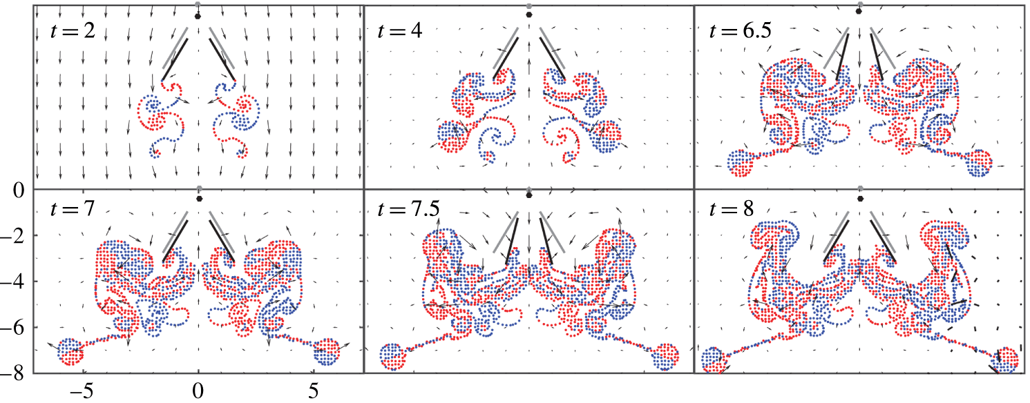
Instantaneous flow velocity field (black arrows) and the wake structure of a hovering flyer with
 $\unicode[STIX]{x1D703}_{a}=0.144,h=1,\unicode[STIX]{x1D703}_{0}=\unicode[STIX]{x03C0}/8$
,
 $d=1$
and
 $M=5$
,
 $I=10$
,
 $R=0.5$
. Positive vortices are coloured in red and negative in blue. For display purposes, the points on the free vortex sheets are coarse grained and plotted as points. Snapshots are at
 $t=2,4,6.5,7,7.5,8$
. The flyer’s initial position is shown in grey as a frame reference. When the background flow is on (
 $t\leqslant 3$
), the flyer sheds dipoles sideways. In the hovering state (
 $t\geqslant 3$
), the flow forms a downward jet inside the body during the power stroke and an upward jet during the recovery stroke. Note that the ‘soup’ of vortices always stays around the wings.

The structure of the free vortex sheets of a hovering flyer is turbulent and complex (see figure 2). To reasonably resolve this structure, we adaptively insert and delete vortices on the free sheets at each time step, such that the distance between adjacent nodes is less than the local smoothing parameter
 $\unicode[STIX]{x1D6FF}$
, and the distance between every other point is greater than
 $0.2\unicode[STIX]{x1D6FF}$
. The position and the strength of any new vortex is extrapolated using the vortices that were generated previously.
Apparently, the number of degrees of freedom of the free vortex sheets (i.e. the number of vortex sheet segment endpoints) increases linearly in time, since at each time step each wing introduces a new vortex into the trailing wake. However, the actual growth is much faster due to the adaptive refinement of the vortex sheets. For a hovering simulation, after six periods of flapping the number of vortices in the free sheets reaches
 $10^{4}$
(using
 $\unicode[STIX]{x0394}t=0.01$
), and after nine periods has reached
 $10^{6}$
. Direct integral summation of the regularized kernel (B 16) is quadratic, which is expensive when the number of vortices becomes large. To ameliorate this cost, in the hovering simulations we use an adaptive kernel-independent fast multipole method (FMM), details of which are shown in appendix C.
4 Simulation results
4.1 Hovering
Our main goal here is to explore theoretically the aerodynamics and stability of hovering flight for a jellyfish-like flyer. The experimental air-jellyfish machine (Ristroph & Childress Reference Ristroph and Childress2014) achieves hovering flight by opening and closing four flapping wings, in a way reminiscent of the swimming motions of a jellyfish. Moreover, the experimental flyer exhibits an intrinsic self-righting stability when its centre of mass is low on the body. This device recovers from excursions to large tilt angles by relying only on its interaction with the surrounding fluid. In this section, we study hovering flight for our theoretical flyer, and its orientational or postural stability (with respect to the tilt angle
 $\unicode[STIX]{x1D6E9}$
). We begin by seeking a left–right symmetric hovering base state
 $(\unicode[STIX]{x1D6E9}(t)=0)$
, upon which we then study the stability in tilt angle
 $\unicode[STIX]{x1D6E9}$
when the flyer undergoes an angular perturbation.
For a hovering flyer initially in a quiescent background flow, i.e.
 $U(t)=0$
, the vortices generated during the first several periods stay close to the wing’s trailing edges. Such initial complex flows at the wing tips make the wing–vortices interaction nearly singular, thus making difficult the accurate evaluation of the boundary integrals. Since our interest is mainly in the dynamics at a ‘steady’ hovering state, for convenience an initial background flow,
 $U(t)=-\!\max (3-t,0)$
, is imposed in the negative
 $y$
-direction. This linearly decreasing uniform flow washes the start-up vortices downstream, and vanishes after three flapping periods.
4.1.1 Seeking a hovering state
In a left–right symmetric hovering state, the average vertical force generated by the wings balances the weight of the flyer. (For simplicity, we use the term ‘lift’ for the period-averaged vertical hydrodynamic force, although this could also be thought of as the thrust produced by the flapping wings. The force generated can be tuned by varying the wing motions, i.e. the flapping amplitude and frequency (Vandenberghe, Zhang & Childress Reference Vandenberghe, Zhang and Childress2004; Vandenberghe, Childress & Zhang Reference Vandenberghe, Childress and Zhang2006)). For our jellyfish-like flyer, when the wing separation
 $d$
and the base opening angle
 $\unicode[STIX]{x1D703}_{0}$
are fixed, the lift produced can then be varied by tuning the flapping amplitude
 $\unicode[STIX]{x1D703}_{a}$
while keeping the flapping frequency unchanged. To find a hovering state, we vary the flapping amplitude
 $\unicode[STIX]{x1D703}_{a}$
and keep other parameters fixed at
 $d=1,\unicode[STIX]{x1D703}_{0}=\unicode[STIX]{x03C0}/8,h=1$
. We find that the flyer maintains a symmetric hovering flight when
 $\unicode[STIX]{x1D703}_{a}\simeq 0.14\sim 0.15({\approx}8.3^{\circ })$
. We select
 $\hat{\unicode[STIX]{x1D703}}_{a}=0.144$
as the condition closest to pure hovering. When
 $\unicode[STIX]{x1D703}_{a}>\hat{\unicode[STIX]{x1D703}}_{a}$
, the lift exceeds the weight so that the flyer rises (ascending flight). For
 $\unicode[STIX]{x1D703}_{a}<\hat{\unicode[STIX]{x1D703}}_{a}$
, the flapping wings are not able to generate enough force to balance the weight and the flyer sinks (descending flight). The speed of ascent and descent depends on the value of
 $|\unicode[STIX]{x1D703}_{a}-\hat{\unicode[STIX]{x1D703}}_{a}|$
.
For hovering with
 $\unicode[STIX]{x1D703}_{a}=\hat{\unicode[STIX]{x1D703}}_{a}=0.144$
, figure 2 and corresponding movie 1 available at https://doi.org/10.1017/jfm.2017.150 show the instantaneous shed vorticity as well as the flow velocity field. While the initial background flow is on, each wing sheds a dipole in one opening–closing stroke (see figure 2 panel for
 $t=2$
). The dipoles convect downwards thereafter with the flow. As the initial flow diminishes and then vanishes, the flyer hovers, and the previous shed dipoles stop convecting and remain close to the flyer (see panel
 $t=4$
). As new vortices are produced continuously from the wing trailing edges, the previously generated vortices merge with the new ones. After about five flapping periods, a complex wake forms below the flyer, being reinforced by absorbing newly generated vortices after each flapping stroke (see figure 2,
 $t\in [6.5,8]$
). As the flyer hovers, the wake lingers around the flyer and it is difficult to resolve numerically. The number of vortices grows superlinearly in time making the computation extremely expensive. In our work, the hovering simulations are performed for
 $10$
flapping strokes, after which the number of vortices has exceeded
 $10^{6}$
and updating one time step takes more than an hour even using FMM.
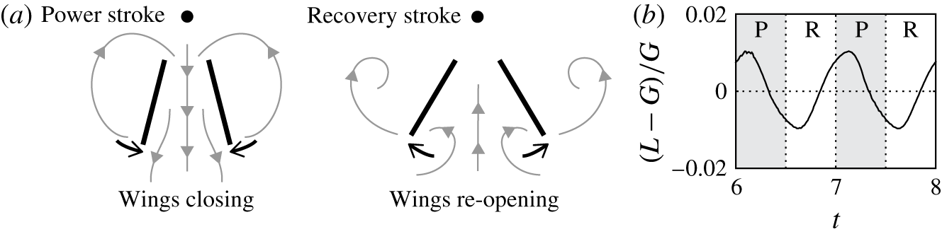
(a) Schematics of the power stroke and the recovery stroke of a free hovering flyer. During the power stroke the wings close, the outer rotational flow is reinforced, and a strong downward jet forms inside the body. During the recovery stroke the wings reopen, the outer wake gets pushed sideways and an upward jet forms inside the flyer body. (b) The lift (
 $L$
) weight (
 $G=2.5$
) difference normalized by the flyer’s weight. In the power stroke (P) the lift is slightly greater than the weight, while in the recovery stroke (R) the lift is slight smaller than the weight. Note that a phase shift exists between the lift and the wing motion.

The hovering flight is depicted schematically in figure 3(a). In the hovering state, each flapping period consists of a power stroke and a recovery stroke. During the power stroke, the wings close inward and positive (negative) vortices are shed outward from the right (left) wing’s tip. These vortices merge with the existing outer wake to form a strong rotational flow around the flyer (see figure 2,
 $t=6.5,7.5$
). This flow moves inside the flyer’s body, through its open top, creating a strong downstream jet that carries momentum downward. The flyer thus gains upward force and the lift so produced is slightly greater than the weight, as shown in figure 3(b). Note that there is a phase shift between the lift and the wing motion. During the recovery stroke, the wings reopen symmetrically (figure 2,
 $t=7,8$
), and the right (left) wing sheds negative (positive) vortices inward while pushing the outer wake further sideways. The inner wake forms a strong upward jet inside the flyer, carrying positive momentum, so that the flyer has a downward momentum while the lift is slightly smaller than the weight (figure 3
b). Therefore, over one cycle of opening and closing the wings, the flyer accelerates and decelerates during the power and recovery stroke. However, the average lift over each beating period generated by the flapping wings balances the weight so that the flyer hovers.
There are other hovering mechanisms related closely to that used by our jellyfish-like flyer. One is the ‘clap-and-fling’ mechanism used by small insects, and studied numerically in two dimensions by Miller & Peskin (Reference Miller and Peskin2005). In 2-D ‘clap-and-fling’, mirror-symmetric wings translate sideways as well as rotate about their leading edges. The fluid dynamics is complicated as during translation vortices are shed from both the leading and trailing edges. For the jellyfish-like flyer, there is no wing translation but only cyclic rotations about their leading edges. This allows us to ignore the leading-edge shedding and to separate the (inwards) power and (outwards) recovery strokes. Another related mechanism is found in experiments and simulations of geometrically anisotropic bodies that hover in vertically oscillating flows (Childress et al. Reference Childress, Vandenberghe and Zhang2006; Spagnolie & Shelley Reference Spagnolie and Shelley2009; Weathers et al. Reference Weathers, Folie, Liu, Childress and Zhang2010; Huang et al. Reference Huang, Nitsche and Kanso2015, Reference Huang, Nitsche and Kanso2016). In the experiments of Weathers et al. (Reference Weathers, Folie, Liu, Childress and Zhang2010) an untethered pyramid with an open bottom (made of paper and wire) was shown to hover when suspended in an oscillating background flow. This hovering could be ascribed to the differences in drag for air passing downwards or upwards along the body. Simulations of these experiments by Huang et al. (Reference Huang, Nitsche and Kanso2015, Reference Huang, Nitsche and Kanso2016) show that this drag anisotropy manifests itself through shed near-dipolar wakes that have some visual similarity to those we observe being generated through the power and recovery strokes. However, unlike the pyramidal hoverer there is no background flow from which to extract energy to generate lift and instead the body must actively change its shape.
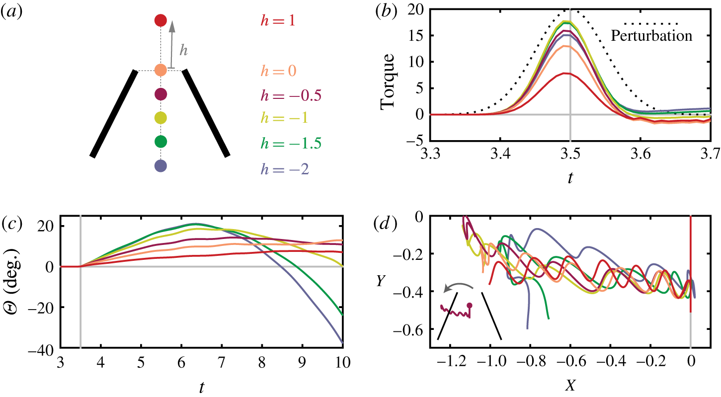
The flyer’s response to a torque impulse
 $E=\unicode[STIX]{x1D716}\exp (-(t-Tc)^{2}/2\unicode[STIX]{x1D70F}_{r}^{2})$
, with
 $\unicode[STIX]{x1D70F}_{r}=0.05,\unicode[STIX]{x1D716}=20$
, at
 $T_{c}=3.5$
. Flyers with centres of mass
 $h=1,0,-0.5,-1,-1.5,-2$
are examined. (a) The schematics for different centre-of-mass locations; (b) combined aerodynamic torque and external torque impulse, compared with the imposed torque (black dotted line); (c) tilt angle dynamics; (d) flyer’s centre-of-mass trajectory. An inset shows the flyer of
 $h=-0.5$
and its trajectory after the perturbation.

4.1.2 Stability of hovering
We study the flyer’s tilt stability in the hovering state by examining the free response of the flyer to an external torque impulse applied during hovering flight. This approach of applying a torque impulse to active flappers has been used previously in experimental studies of the autostabilization of fruit flies (Ristroph et al.
Reference Ristroph, Bergou, Ristroph, Coumes, Berman, Guckenheimer, Wang and Cohen2010). For hovering flight
 $(\unicode[STIX]{x1D703}_{a}=0.144)$
with
 $t>3$
(when the initial background flow has vanished), we impose a torque perturbation as follows. In the angular momentum equation, (2.8), a Gaussian perturbation term is added,
 $$\begin{eqnarray}I\ddot{\unicode[STIX]{x1D6E9}}=\mathop{\sum }_{k=1,2}\int _{C_{k}^{b}}(\boldsymbol{x}_{k}-\boldsymbol{X})^{\bot }\cdot [p_{k}]\hat{\boldsymbol{n}}_{k}\,\text{d}s+T_{p}(t).\end{eqnarray}$$
The perturbation
 $$\begin{eqnarray}T_{p}(t)=\unicode[STIX]{x1D716}\exp (-(t-t_{c})^{2}/2\unicode[STIX]{x1D70F}_{c}^{2})\end{eqnarray}$$
is a Gaussian impulse form centred at
 $t_{c}=3.5$
. The impulse has an amplitude
 $\unicode[STIX]{x1D716}=20$
and a width
 $\unicode[STIX]{x1D70F}_{c}=0.05$
, and lasts only approximately
 $0.3$
of a flapping period. As the Gaussian torque impulse is imposed, a total external angular momentum of
 $\sqrt{2\unicode[STIX]{x03C0}}\unicode[STIX]{x1D716}\unicode[STIX]{x1D70F}_{c}$
is added to the flyer. We examine the free response of flyers with the centre of mass located at different positions in the body, i.e.
 $h=1,0,-0.5,-1,-1.5,-2$
, as shown in the schematic of figure 4(a).
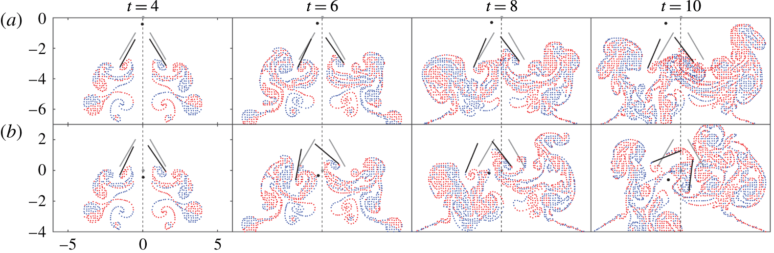
As the external torque is applied to the flyer, the fluid generates a strong aerodynamic resistive torque. Figure 4(b) shows that the net torque on the flyer, a combination of the imposed torque and the aerodynamic torque, is less than the torque imposed. This indicates that part of the external angular momentum added into the system has dissipated in the fluid, so that the impulse is damped and the flyer is prevented from tilting to a large angle. After the impulse, 40 % of the added torque has dissipated into the fluid for the bottom-heavy flyer with
 $h=-2$
, and 75 % for the top-heavy flyer with
 $h=1$
. It seems that the top-heavy flyers tend to generate more resistance to the impulse. This is not surprising as the top-heavy flyers have longer torque arms (the distance between the centre of mass and the flyer’s geometric centre), so that a small sideways force can be amplified to a large resistive torque.
After the torque impulse is applied, when
 $t\in [4,6]$
, the flyer tilts and translates sideways; see figure 4(c,d). The tilt angle of the top-heavy flyers increases more slowly than the bottom-heavy flyers, since more of the external torque is absorbed by the fluid. The translational motion is presumably due to the sideways component of the aerodynamic force generated along the flyer’s axis, which is in the same direction as the flyer’s orientation
 $\unicode[STIX]{x1D6E9}$
. Although the sideways motion is weak – the flyers typically migrate only half the wing length in approximately seven periods – the translational motion again causes a sideways wing drag that in turn rotates the flyer.
At time
 $t\approx 6.5$
, when the tilt angle of bottom-heavy flyers with
 $h=-1.5$
and
 $-2$
has reached
 ${\sim}20^{\circ }$
, the flyer starts to recover (see figure 4
c and movie 2). Such self-righting behaviour of bottom-heavy flyers is intrinsic, as it does not arise from any external stabilizing mechanisms and relies only on the aerodynamics on the flyer. The recovery is due to the complex, coupled rotational and translational motions of the flyer. For bottom-heavy flyers (
 $h=-1.5,-2$
), the flyer’s geometric centre (the point the aerodynamic force acts) is above the centre of mass (the point at which gravity acts). In this case, the torque induced by the sideways drag acts as a restoring torque, and we believe this causes the flyer to turn. However, at times
 $t\geqslant 9$
when the bottom-heavy flyers (
 $h=-1.5$
and
 $-2$
) have reached a large tilt in the other direction, the self-righting behaviour does not occur, and the flyer eventually flips over into the wake (see figure 5 and movie 2). The wake structure shows that when
 $t\geqslant 9$
the flyer’s right wing is sucked by the rotational flow outside the body and the counter-rotational flow inside the body. A strong torque caused by the flow asymmetry thus prevents the flyer from recovering. As the flyer tilts largely to the right, the flyer also drops vertically, as the trajectory shows in figure 4(d). It is because the vertical component of the flyer’s axial force decreases as the tilt angle increases, leading to insufficient vertical force to balance the flyer’s weight.
The top-heavy flyers, say with
 $h=1$
and
 $0$
, are unstable but very weakly so, and the tilt angle
 $\unicode[STIX]{x1D6E9}$
increases slowly as the flyer translates sideways. For example, within
 $10$
periods of the simulation, the tilt angle of the top-heavy flyers reaches only
 ${\sim}10^{\circ }$
. We think the main reason that the top-heavy flyers rotate so slowly is because a large portion of the added torque is absorbed by the flow (figure 4
b). This leads to less perturbed flow structures and more symmetric aerodynamic force on both wings (see figure 5 for
 $h=1$
and movie 3).
In summary, bottom-heavy flyers return to the upright position for short times, a behaviour called static stability in the airplane flight dynamics literature (Stengel Reference Stengel2015). However, these flyers overshoot the upright position, suggesting that the body rotations may diverge in time, in which case the flyer is said to be dynamically unstable. Top-heavy flyers, on the other hand, display a slowly diverging orientation angle, which is consistent with static and dynamic instability. For all flyers, we note that our simulations cannot assess the long-time stability because of the limitations in the simulation run time. For intermediate centre-of-mass locations, the flyers may in fact be dynamically stable, but a longer running simulation would be required to evaluate this.
Responses of (a) a top-heavy flyer
 $h=1$
and (b) a bottom-heavy flyer
 $h=-2$
to an external torque perturbation. Positive vortices are coloured in red and negative in blue. Points on the free vortex sheets are coarse-grained and displayed using points. Snapshots are at time
 $t=4,6,8,10$
. The flyer’s initial position is presented in grey. After the impulse, the top-heavy flyer tilts slightly and then the angle keeps increasing slowly, while the bottom-heavy flyer tilts to a large angle, comes back upright and then overshoots.

4.2 The ascending state
If the flapping amplitude is increased such that
 $\unicode[STIX]{x1D703}_{a}>\hat{\unicode[STIX]{x1D703}}_{a}$
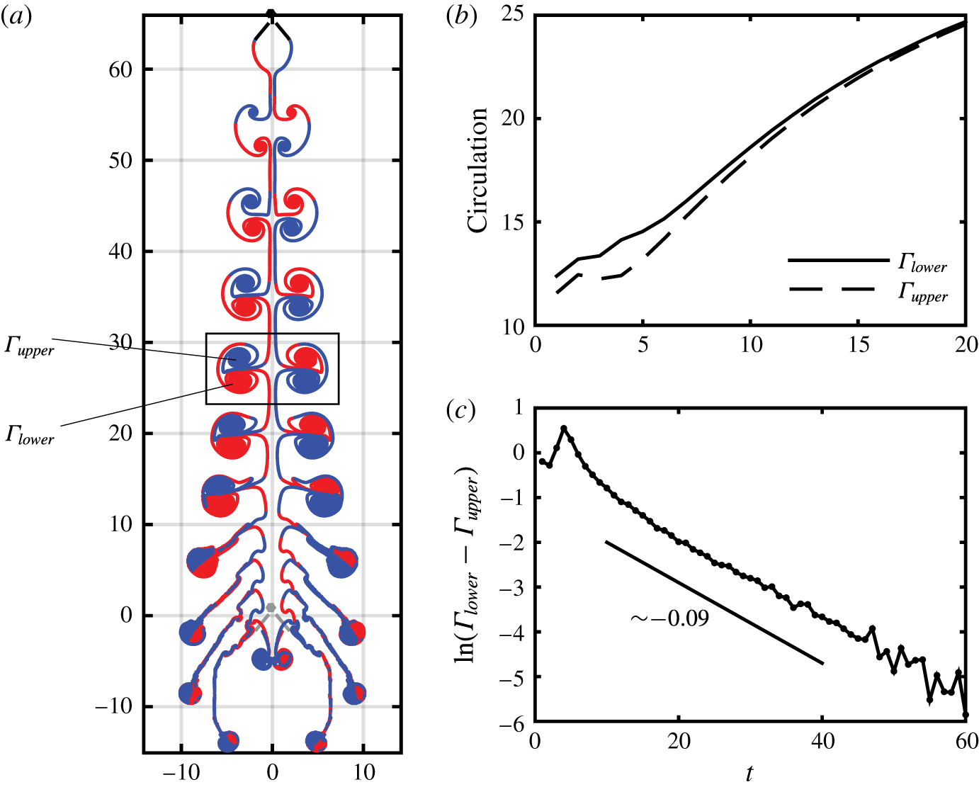
, the flyer’s lift exceeds its weight, and it ascends upward (movie 4). As the flyer ascends, the body leaves a clear wake structure behind it, as shown in figure 6(a). During accelerating ascent flight, the flyer sheds one vortex quadrupole in every flapping stroke. The quadrupole consists of two left–right ‘near-dipoles’. A near-dipole is a weakly asymmetric dipole in which the two constituent vortices are of different intensity. Due to their unbalanced strength, an isolated near-dipole rotates in addition to translating, leading to a curved trajectory (Saffman Reference Saffman1993). In our case, the strength of vortices in the near-dipole is calculated as the circulation of vortex sheet pieces of the same sign. As displayed in figure 6(a), we denote by
 $\unicode[STIX]{x1D6E4}_{upper}$
the circulation of the vortex sheet section of negative (positive) strength generated by the left (right) wing, as coloured in blue (red), and denote by
 $\unicode[STIX]{x1D6E4}_{lower}$
the circulation of the vortex sheet section of positive (negative) strength shed by the left (right) wing. Note that
 $\unicode[STIX]{x1D6E4}_{upper}$
and
 $\unicode[STIX]{x1D6E4}_{lower}$
are functions of time, denoting the strength of the near-dipoles generated at each flapping stroke. As the flyer accelerates, the lower vortex, which is generated in the closing or power stroke, is always slightly stronger than the upper vortex generated in the opening or recovery stroke, i.e.
 $\unicode[STIX]{x1D6E4}_{lower}>\unicode[STIX]{x1D6E4}_{upper}$
, see figure 6(b,c). Such asymmetric strength causes the near-dipole to move downwards, in addition to moving sideways. The downward motion of the near-dipoles carries downward momentum, and the flyer experiences an upward force as a result.
The flyer takes off when
 $\unicode[STIX]{x1D703}_{a}=0.3>\hat{\unicode[STIX]{x1D703}}_{a}$
. (a) The wake structure of the flyer’s ascending take-off, when
 $t=11$
. Each stroke generates one vortex quadrupole, consisting of two symmetric near-dipoles. Within the near-dipoles,
 $\unicode[STIX]{x1D6E4}_{upper}$
and
 $\unicode[STIX]{x1D6E4}_{lower}$
denote the circulation (strength) of the upper and lower vortices respectively. The near-dipoles move sideways and also downwards, leading to curved trajectories. The flyer’s initial position is shown in grey. (b) Circulation of vortices in the near-dipoles. Lower vortex circulation
 $\unicode[STIX]{x1D6E4}_{lower}$
is always greater than the upper
 $\unicode[STIX]{x1D6E4}_{upper}$
. (c) Circulation difference in near-dipoles, on a logarithmic scale. The difference decays exponentially in time as
 $\unicode[STIX]{x1D6E4}_{lower}-\unicode[STIX]{x1D6E4}_{upper}\sim \text{e}^{-0.09t}$
.

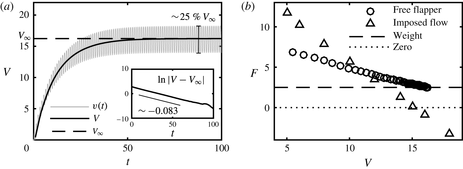
In these ascent simulations, we replace the far-field vortex sheets using point vortices (Alben Reference Alben2009), allowing us to perform long-time simulations efficiently. The long-time simulation reveals a stroke-averaged steady ascent. That is, the flyer’s period-averaged ascending velocity,
 $V(t)=\langle v\rangle =\int _{t}^{t+1}v(t^{\prime })\,\text{d}t^{\prime }$
, approaches a terminal speed
 $V_{\infty }$
, where
 $v(t)$
is the instantaneous vertical velocity of the flyer (see figure 7
a). For
 $\unicode[STIX]{x1D703}_{a}=0.3$
, the instantaneous velocity
 $v(t)$
attains a mean of
 $V_{\infty }\approx 16.22$
and oscillates with a peak-to-peak amplitude of
 $25\,\%$
. This steady state seems to be unique: starting the flyer from different initial conditions yields the same terminal speed. When the steady state is reached, the stroke-averaged aerodynamic force
 $F$
and the flyer’s weight come into balance (figure 7
b). The quadrupoles are now composed of symmetric dipoles of equal strength, i.e.
 $\unicode[STIX]{x1D6E4}_{lower}=\unicode[STIX]{x1D6E4}_{upper}$
, as no mean downward fluid momentum is generated when the flyer reaches its steady speed. The trend of
 $\unicode[STIX]{x1D6E4}_{lower}-\unicode[STIX]{x1D6E4}_{upper}\rightarrow 0$
as
 $t\rightarrow \infty$
is displayed in figure 6(c).
Dynamics of ascent. (a) The flyer’s instantaneous ascent speed
 $v(t)$
and its stroke average
 $V$
. A time-averaged ascent speed
 $V_{\infty }\approx 16.22$
is approached exponentially in time, as the inset shows
 $|V-V_{\infty }|\sim \text{e}^{-0.083t}$
. At steady state
 $v(t)$
fluctuates with an amplitude of approximately
 $25\,\%$
of the mean
 $V_{\infty }$
. (b) The aerodynamic force
 $F$
on the free ascending flyer is linear in ascent speed
 $V$
, and approaches the weight at steady state. The aerodynamic force
 $F$
on the flyer with an imposed ascent speed
 $V$
is linear in the speed. Both results show the linear force–speed relationship of the active flyer.

The flyer’s period-averaged ascent speed
 $V(t)$
approaches the steady speed
 $V_{\infty }$
exponentially in time (figure 7
a), and the near-dipole strength difference
 $\unicode[STIX]{x1D6E4}_{lower}-\unicode[STIX]{x1D6E4}_{upper}$
also decays exponentially, which implies the momentum generation diminishes with an exponential rate (figure 6
c). This exponential relaxation to the steady state implies a linear relationship between the aerodynamic force
 $F$
and ascent speed
 $V$
(figure 7
b),
 $$\begin{eqnarray}M\dot{V}=F-M\mathit{Fr}^{-2},~\text{where}~F=-C_{1}V+C_{0}.\end{eqnarray}$$
Here
 $C_{1}$
and
 $C_{0}$
are constants whose values are calculated by fitting the
 $F-V$
curve in figure 7(b) linearly. Note that
 $C_{1}$
determines a time scale of system relaxation
 $\unicode[STIX]{x1D70F}=M/C_{1}$
, as the solution to (4.3) is
 $V=V_{\infty }(1-\text{e}^{-t/\unicode[STIX]{x1D70F}})$
. For the simulation shown here (
 $\unicode[STIX]{x1D703}_{a}=0.3$
), the time scale is found to be
 $\unicode[STIX]{x1D70F}=11\sim 12$
.
To further investigate the force–speed relationship, we impose on the flyer a fixed ascent speed
 $V$
, and measure the aerodynamic force
 $F$
when the system reaches steady state. In the flyer’s frame this is equivalent to fixing an active flapping flyer in a wind tunnel, where the flyer’s centre of mass is fixed in place and the flyer is immersed in a uniform downward background flow of speed
 $V$
. A linear relation between the aerodynamic force
 $F$
and the imposed speed
 $V$
is found yet again, as shown in figure 7(b). However, note that the free flight forces are different from those experienced in the imposed flow, a topic we take up in the discussion section § 5.
4.2.1 Results with respect to variation of physical parameters
We consider the effect of two physical parameters on ascent dynamics and steady states, the flapping amplitude
 $\unicode[STIX]{x1D703}_{a}$
and wing separation distance
 $d$
, with the main quantities of interest being the steady ascent speed
 $V_{\infty }$
and the Froude efficiency
 $\unicode[STIX]{x1D702}=\langle P_{out}\rangle /\langle P_{in}\rangle$
, calculated by (2.10)–(2.12).
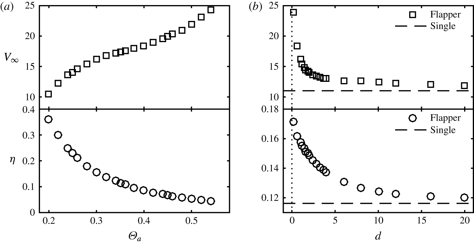
The effect of varying physical parameters on the steady ascent speed
 $V_{\infty }$
and Froude efficiency
 $\unicode[STIX]{x1D702}$
(2.12). (a) Varying flapping amplitude
 $\unicode[STIX]{x1D703}_{a}$
. (b) Varying wing separation
 $d$
. Results are compared with a single pitching wing that has the same flapping motion and supports half of the flyer’s mass (dashed line), which can be considered as representing the case of
 $d=\infty$
.

We begin by examining the result of varying the flapping amplitude
 $\unicode[STIX]{x1D703}_{a}$
. We fix the flyer’s base opening angle to be
 $\unicode[STIX]{x1D703}_{0}=\unicode[STIX]{x03C0}/8\approx 0.39$
, and we examine the flapping amplitude in the range of
 $\unicode[STIX]{x1D703}_{a}\in [0.2,0.54]$
, and show the results in figure 8(a). (Smaller
 $\unicode[STIX]{x1D703}_{a}$
does not generate ascent and larger
 $\unicode[STIX]{x1D703}_{a}$
values would cause the wings to collide.) As the flapping amplitude
 $\unicode[STIX]{x1D703}_{a}$
increases, the steady ascent velocity increases monotonically in
 $\unicode[STIX]{x1D703}_{a}$
. This is consistent with previous studies of self-propelled flapping wings which have shown the swimming speed is an increasing function of flapping speed (Vandenberghe et al.
Reference Vandenberghe, Zhang and Childress2004; Alben & Shelley Reference Alben and Shelley2005; Vandenberghe et al.
Reference Vandenberghe, Childress and Zhang2006). The Froude efficiency
 $\unicode[STIX]{x1D702}$
decreases dramatically as
 $\unicode[STIX]{x1D703}_{a}$
increases. This may be because larger amplitudes accelerate the fluid more outwardly rather than downwardly.
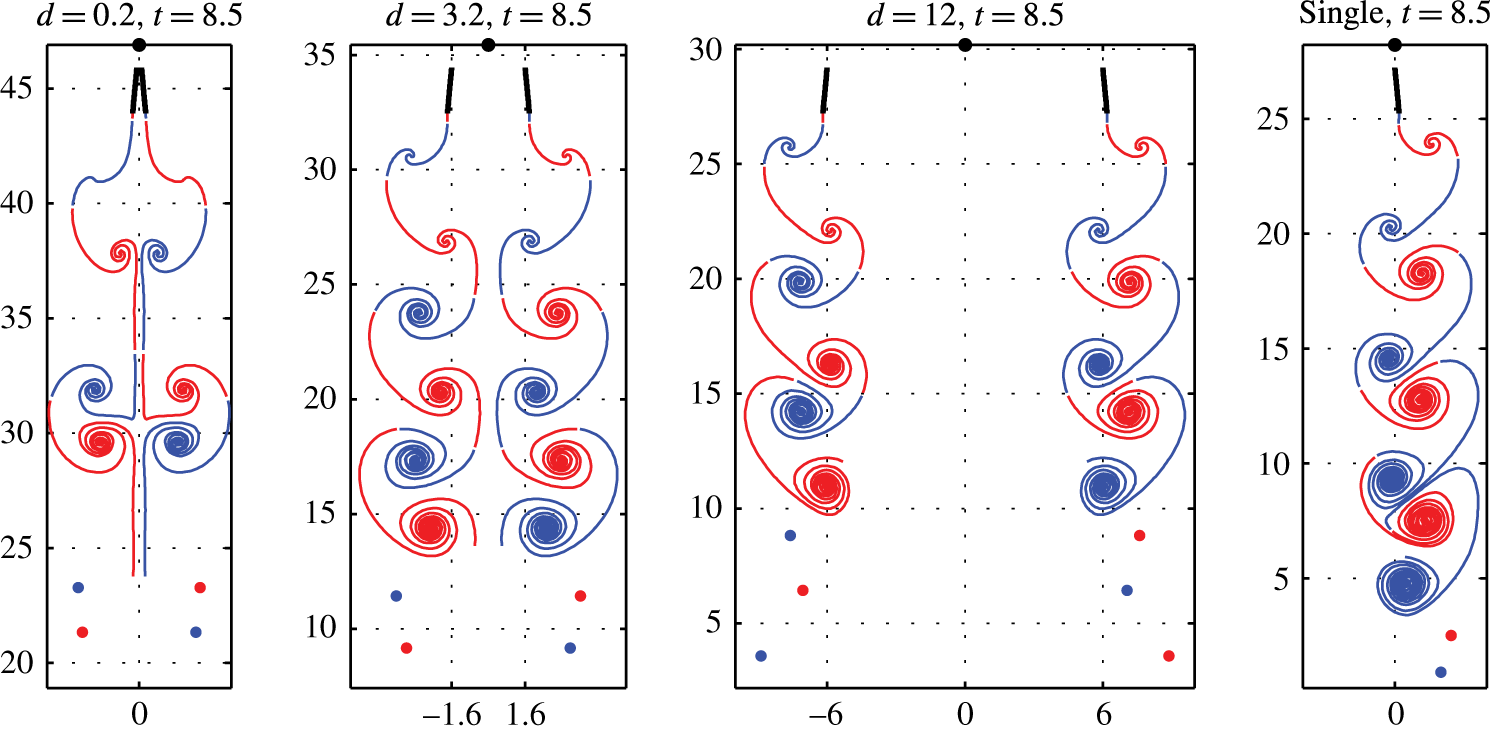
The instantaneous wake structure of flyers with wing separation
 $d=0.2,~3.2,~12$
and the wake structure of a single skewed pitching wing. The single wing has the same pitching motion as the right wing of the flyer and supports half of the flyer’s mass, which can be considered as representing
 $d=\infty$
. Snapshots are taken at
 $t=8.5$
, where
 $\unicode[STIX]{x1D703}_{a}=0.3$
. The far-field vortex sheets are approximated using point vortices.

We now consider the wing separation distance
 $d$
, as shown in figures 9 and 8(b). When
 $d$
is small (for example
 $d=0.2$
in figure 9), the wings are close, the interactions between symmetric left–right wings and their vortex sheets are strong. The separation between successive quadrupoles is large so that the vortex interaction is dominated by the quadrupole self-interaction. Within a wake quadrupole, the symmetric left–right near-dipoles are repelled and move sideways shortly after being generated from their wing tips. As
 $d$
increases (
 $d=3.2$
in figure 9), the quadrupole wake pattern becomes more compressed vertically. In this case, the flyer generates two mirror-symmetric skewed inverse von Kármán streets, and each vortex interacts strongly with vortices on its own street and on the other street. As
 $d$
is incrementally varied (
 $d=12$
in figure 9), the two vortex streets are well separated. The skewed inverse von Kármán street shed by each wing resembles the vortex street generated by a single pitching wing, as expected. Here the single wing is prescribed with the same pitching motion as the flyer’s right wing, which models a half of the flyer with
 $d=\infty$
. The single wing is free to ascend in the vertical direction and supports
 $1/2M$
mass.
Figure 8(b) shows how the ascent performance is affected by
 $d$
. We see that the steady ascent velocity
 $V_{\infty }$
and the efficiency
 $\unicode[STIX]{x1D702}$
are both increased as
 $d$
is reduced, and interactions between symmetric wings and wake get stronger. By reducing
 $d$
from
 $\infty$
to
 $0$
, the ascent speed is doubled and the efficiency is increased by
 $50\,\%$
, compared to
 $d=\infty$
. This increased interaction of the wings about their symmetry plane is reminiscent of ‘ground effect’. One recent study by Quinn et al. (Reference Quinn, Moored, Dewey and Smits2014) examined experimentally an airfoil pitching near a solid boundary but otherwise held against a background flow, and also simulated the corresponding computational problem of two mirror image pitching airfoils. They find that thrust increases as the airfoil separation distance decreases, and that the Strouhal number (
 $\mathit{St}=fa/u_{\infty }$
with
 $f$
the pitching frequency,
 $a$
the peak-to-peak amplitude of pitching, and
 $u_{\infty }$
the free-stream speed) decreases as a defined ‘propulsive efficiency’ increases. While in our case the velocity is chosen by the wing dynamics, their results are nonetheless consistent in that the speed increases with decreasing wing separation, which yields both decreased Strouhal number (using the ascent velocity as the free-stream speed) and increased efficiency
 $\unicode[STIX]{x1D702}$
.
4.2.2 Stability of the ascending state
Finally, we examine the flyer’s stability during ascent. Like the hovering stability study, we consider the flyer’s free response to an external Gaussian torque impulse
 $T_{p}(t)=\unicode[STIX]{x1D716}\exp (-(t-t_{c})^{2}/2\unicode[STIX]{x1D70F}_{c}^{2})$
, via (4.1), after the flyer has reached an ascending steady state. Flyers with their centre of mass located at
 $h=-2,-1.5,-1,-0.5,0,1$
(shown in figure 4
a) are examined. Here we have used
 $\unicode[STIX]{x1D6E9}_{a}=0.3$
and wing separation
 $d=1$
. We initialize the ascent speed near the terminal speed, and apply the perturbation at
 $t_{c}=13.5$
when the speed is within
 $10\,\%$
of the terminal speed. Specifically, we impose a Gaussian torque perturbation centred at time
 $t_{c}=13.5$
and with width of
 $\unicode[STIX]{x1D70F}_{c}=0.05$
, so that the impulse lasts only approximately 0.3 flapping periods.
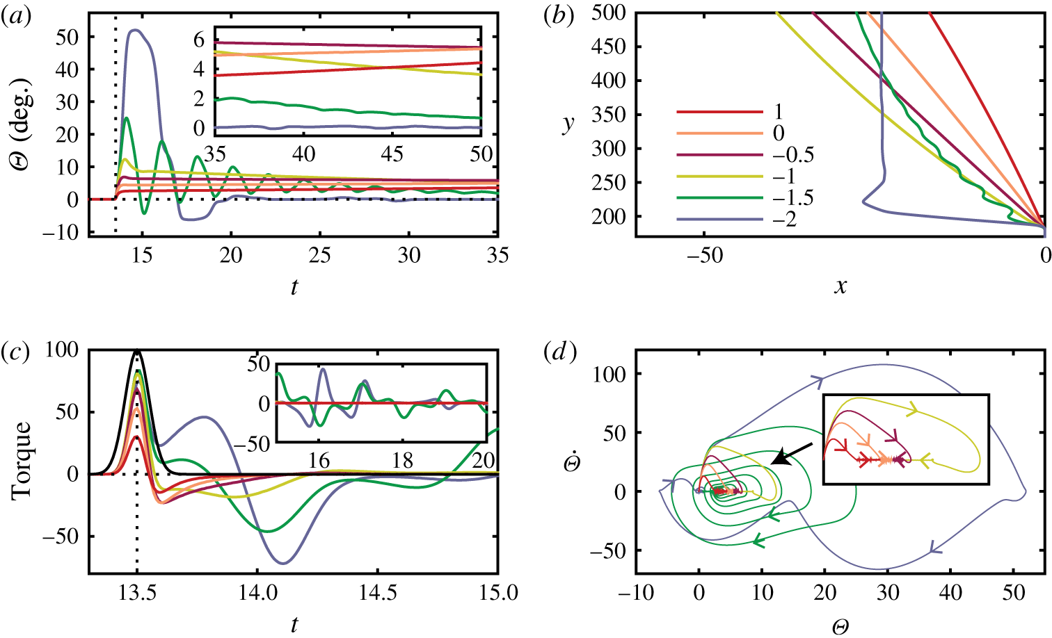
The flyer’s free response to a torque impulse during ascending steady state. An impulse of strength
 $\unicode[STIX]{x1D716}=100$
is applied at
 $t_{c}=13.5$
. The flyers of centre of mass
 $h=-2,-1.5,-1,-0.5,0,1$
are examined for
 $t\in [0,50]$
. (a) The tilt angle
 $\unicode[STIX]{x1D6E9}$
. The inset shows
 $t\in [35,50]$
. (b) The flyers’ paths after the torque perturbation. (c) The torque impulse
 $T_{p}(t)$
(black curve) and the net torque on the flyer (coloured curves). The inset shows
 $t\in [15,20]$
. (d) A phase space plot for tilt dynamics.

The flyer’s response to a perturbation of strength
 $\unicode[STIX]{x1D716}=100$
is shown in figure 10. The impulse is stronger than that used in the hovering stability study, where
 $\unicode[STIX]{x1D716}=20$
, because during an ascending flight the relative fast background flow provides a stronger restoring torque when the perturbation is applied. For the centre-of-mass locations
 $h$
we investigate, three types of ascent stability are found. The top-heavy flyers with
 $h\in [-1,1]$
generate a strong resistive aerodynamic torque when the external torque is applied at
 $t\in [13.3,13.7]$
, leading to a small net torque on the flyer (figure 10
c). The flyer then tilts slightly towards one side (figure 10
a). Within one period after the impulse, the tilt angle reaches a maximum value
 $\unicode[STIX]{x1D6E9}_{max}=\max _{t\in [13.7,14.7]}\unicode[STIX]{x1D6E9}(t)<13^{\circ }$
(shown in figure 10
a). After approximately one flapping period after the impulse has vanished (
 $t\geqslant 15$
), the tilt angle
 $\unicode[STIX]{x1D6E9}$
changes (increases or decreases) steadily in time, and the period-averaged angular velocity
 $\langle \dot{\unicode[STIX]{x1D6E9}}\rangle =\int _{t}^{t+1}\dot{\unicode[STIX]{x1D6E9}}(t^{\prime })\,\text{d}t^{\prime }$
is nearly constant. The angle of the most top-heavy flyers (
 $h=0$
or
 $1$
) increases steadily, while the angle of flyers with
 $h=-1,-0.5$
decreases steadily. The linear growth rate of the stroke-averaged tilt angle,
 $\unicode[STIX]{x1D706}=\langle \dot{\unicode[STIX]{x1D6E9}}\rangle /\langle \unicode[STIX]{x1D6E9}\rangle$
, is averaged over
 $t\in [20,50]$
, and denoted by
 $\overline{\unicode[STIX]{x1D706}}$
as shown in figure 11(a). A mathematical justification of the linear growth rate is shown in appendix D. Although the angle of the top-heavy flyers,
 $h=0$
or
 $1$
, diverges steadily, the growth rate is very small and the top-heavy flyers can be considered weakly unstable (angle increment is less than
 $1^{\circ }$
every
 $20$
flapping periods). Figure 11(a) also shows a bifurcation point at
 $h_{c}\approx -0.3$
in centre-of-mass location
 $h$
. For flyers with
 $h\in [h_{c},1]$
, the tilt angle diverges slowly after the impulse, and for flyers with
 $h\in [-1,h_{c}]$
, the angle converges and the flyer recovers steadily to the upright orientation.
For bottom-heavy flyers with
 $h=-1.5$
and
 $-2$
, the aerodynamic resistive torque is weak when the impulse is applied, resulting in a large net tilting torque on flyers (figure 10
c). Unlike the top-heavy ones, when
 $t\in [13.6,13.9]$
the bottom-heavy flyers feel another strong tilting torque soon after the impulse. Both the weak resistive torque and the post-impulse torque make the bottom-heavy flyers turn to large angles soon after the perturbation. In one period after the perturbation, the flyer with
 $h=-1.5$
reaches a maximal angle
 $\unicode[STIX]{x1D6E9}_{max}\approx 25^{\circ }$
and the flyer of
 $h=-2$
reaches
 $\unicode[STIX]{x1D6E9}_{max}\approx 52^{\circ }$
(figure 10
a). After the impulse, the two flyers present different recovery dynamics. The tilt angle of the flyer of
 $h=-1.5$
oscillates and converges to zero, with an oscillation time scale of approximately two flapping strokes. After approximately
 $31$
flapping periods after the impulse when
 $t\geqslant 45$
, the angle
 $\unicode[STIX]{x1D6E9}$
reaches a value less than
 $1^{\circ }$
. The other bottom-heavy flyer
 $h=-2$
, unlike the flyers discussed before, recovers from the large tilt
 $\unicode[STIX]{x1D6E9}_{max}\approx 52^{\circ }$
to the upright orientation quickly in approximately five flapping periods (figure 10). The angle satisfies
 $|\unicode[STIX]{x1D6E9}(t)|\leqslant 1^{\circ }$
when
 $t\geqslant 21$
, about seven flapping periods after the impulse.
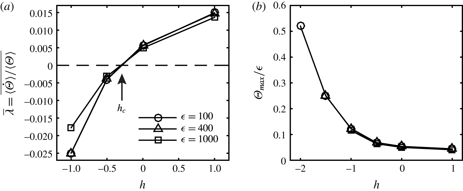
(a) For flyers with
 $h\in [-1,1]$
, the linear growth rate
 $\unicode[STIX]{x1D706}$
of the stroke-averaged tilt angle
 $\langle \unicode[STIX]{x1D6E9}\rangle$
is averaged over
 $t\in [20,50]$
, denoted by
 $\overline{\unicode[STIX]{x1D706}}$
. A stability bifurcation point is denoted at
 $h_{c}\approx -0.3$
. The growth rate is intrinsic to flyers as it is independent of the impulse strength
 $\unicode[STIX]{x1D716}$
. (b) The maximum tilt angle in one period after the torque impulse (
 $t\in [13.7,14.7]$
) normalized by
 $\unicode[STIX]{x1D716}$
. Bottom-heavy flyers turn over in strong perturbations, resulting in missing data for
 $h=-2,~\unicode[STIX]{x1D716}=400$
or
 $1000$
and
 $h=-1.5,~\unicode[STIX]{x1D716}=400$
. Fixing
 $h$
, the maximum angle
 $\unicode[STIX]{x1D6E9}_{max}$
is proportional to perturbation strength
 $\unicode[STIX]{x1D716}$
.

Next, we show that the ascent stability seems to be an intrinsic property of the flyer, which depends on the centre-of-mass location
 $h$
but not on the perturbation. In particular, for a flyer of fixed
 $h$
, the stability properties do not change as
 $\unicode[STIX]{x1D716}$
is increased, as long as the flyer is not turned over by the impulse. For flyers with
 $h\in [-1,1]$
, the linear growth rate is found to be independent of the perturbation strength
 $\unicode[STIX]{x1D716}$
, as shown in figure 11(a). Moreover, the flyer’s response to the perturbation is proportional to the impulse strength
 $\unicode[STIX]{x1D716}$
. Figure 11(b) shows data of the post-impulse maximal tilt
 $\unicode[STIX]{x1D6E9}_{max}$
, and the data collapse when normalized by
 $\unicode[STIX]{x1D716}$
. For
 $\unicode[STIX]{x1D716}=400$
, the flyer of
 $h=-2$
is turned over quickly by the external impulse as the tilt angle exceeds
 $180^{\circ }$
at
 $t=14.1$
. A similar turning over occurs for both
 $h=-2$
and
 $h=-1.5$
when
 $\unicode[STIX]{x1D716}=1000$
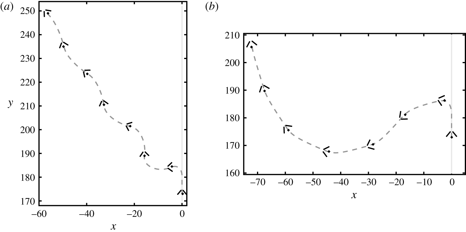
. The free recovery flight of a bottom-heavy flyer with
 $h=-1.5$
after an impulse of strength
 $\unicode[STIX]{x1D716}=400$
, and the recovery of
 $h=-2$
after an impulse
 $\unicode[STIX]{x1D716}=200$
are displayed in figure 12 and movies 5 and 6. Under an impulse of
 $\unicode[STIX]{x1D716}=200$
, the bottom-heavy flyer
 $h=-2$
undergoes an extreme tilt to an angle of
 $\unicode[STIX]{x1D6E9}_{max}=137^{\circ }$
, but after the impulse it recovers back to the upright orientation after several flapping periods due to the intrinsic stability.
Free recovery flight of two bottom-heavy flyers
 $h=-1.5$
(a) and
 $h=-2$
(b) for
 $t\in [13,20]$
. An external torque perturbation is applied at
 $t_{c}=13.5$
during the steady ascending state of the flyer. The snapshots are taken at the beginning of each flapping period,
 $t=13,14,\ldots ,20$
. The grey dashed line shows the flyer’s trajectory in
 $t\in [13,20]$
. (a)
 $h=-1.5$
and
 $\unicode[STIX]{x1D716}=400$
. (b)
 $h=-2$
and
 $\unicode[STIX]{x1D716}=200$
.

5 Conclusion and discussions
We have studied a 2-D mathematical jellyfish-like flyer using a vortex-sheet-based simulation method. We find that the flyer is able to hover and ascend freely, where these simple manoeuvres are achieved through adjusting flapping-wing amplitude. We find that a time-averaged steady ascent state is approached exponentially in time, during which the aerodynamic force is a linear function of the speed. We have varied the flapping amplitude of the wings and the wing separation to study how they influence the performance of ascending flight. We find that the steady ascent speed is strongly correlated with the flapping amplitude but efficiency is inversely correlated, whereas both the speed and efficiency increase as the wings are brought closer together due to a symmetric ‘ground effect’. These results provide us with insights for engineering designs of future jellyfish-like ornithopters which could be both manoeuvrable and efficient, and our study implies this might be achieved through a cooperative adjustment of the flapping amplitude, flapping frequency, the wing separation and centre-of-mass position.
We have incorporated the FMM into the vortex sheet simulation. Implementing FMM allows us to simulate
 $10$
flapping strokes of hovering flight, where the complex fluid wake is composed of
 $10^{6}$
vortices on the free vortex sheets. In hovering simulations, the vortex sheets cannot be coarse grained simply using point vortices, because the wake lingers close to the flyer. Therefore, as the number of vortices on the vortex sheets grows linearly in time, longer time simulations of hovering become very challenging due to the expensive computational cost, and thus we are not able to definitively evaluate the long-time hovering stability. To improve the method, the free vortex sheets need to be coarse grained properly in order to reduce the number of degrees of freedom. Appropriate kernel regularization might also be necessary for stabilities, and robust quadrature rules could be developed accordingly. Another approach would be to not shed a vortex at every time step, but less frequently while still maintaining the smoothness of the flow near the wings’ trailing ends; see the work of (Michelin, Smith & Glover Reference Michelin, Smith and Glover2008).
The time-averaged steady ascent state is found to be approached exponentially in time, and the aerodynamic force
 $F$
is a linear function of the stroke-averaged ascent speed
 $V$
. This linear force–speed relationship is found in both freely ascending flyers and flyers held in an imposed flow. The coefficient relating force and speed, however, is different in these two cases, as shown in figure 7(b), which indicates that the oscillations in ascent speed
 $v(t)$
within a stroke affect the dynamics. This difference highlights the importance of modelling the true free flight dynamics where the body and wing motions are coupled instantaneously to the fluid flows.
The experiments and simulations have a number of differences that might be expected to lead to differences in flight dynamics and flyer stability. Perhaps most importantly, the model is two-dimensional while the experiment is (obviously) three-dimensional (Ristroph & Childress Reference Ristroph and Childress2014). We note that when the experimental 3-D flyer hovers it can leave behind its wake by moving around in a horizontal plane. In our 2-D model, the flyer is much more constrained in how it can escape the complex flows generated during hovering. This particular aspect makes simulating long-time hovering dynamics difficult. Moreover, the experimental flyers have wings which bend elastically as they are flapped, which is not captured in our model. Further, the wing mass comprises a significant portion of the total mass of the experimental flyer, while we concentrate the mass into a virtual centre of mass.
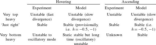
Nonetheless, we have studied the postural stability during hovering and ascent, and our results compare quite well with experimental observations (Ristroph & Childress Reference Ristroph and Childress2014). Some of these comparisons are summarized in table 1. Firstly, the experiments found very top-heavy flyers to be unstable both during hovering and in ascending flight. Our simulations show that while such flyers generate a strong and immediate resistive torque, the flyer orientation ultimately shows a slow divergence. Thus both experiments and simulations suggest the very top-heavy flyers are subject to eventual postural instability. For very bottom-heavy flyers, experiments showed instability to oscillatory model during hovering (personal communications). Simulations show that such flyers generate a weak and immediate resistive torque to an orientation perturbation in both hovering and ascent. In hovering, the flyers will return towards the upright position, perhaps with overshoot, which is consistent with static stability but may also reflect a slow oscillatory instability. Unfortunately, computational limitations prevented us from investigating this dynamics further in time. Thus experiments and simulations both show that the hovering of very bottom-heavy flyers is oscillatory unstable. During ascent, the simulations of very bottom-heavy flyers show a robust upright stability, while experiment results are not known from Ristroph & Childress (Reference Ristroph and Childress2014). Finally, as in the experiments we also find a region of ‘just right’ flyers, in particular with
 $h=-0.5$
and
 $-1.0$
where the flyer shows postural stability both while hovering (provisionally, given the limited computation time) and ascending.
Qualitative stability comparisons of the model flyer with experimental flyer (Ristroph & Childress Reference Ristroph and Childress2014).

Our hovering stability simulations can also be compared to the linear model in Ristroph & Childress (Reference Ristroph and Childress2014), in which the aerodynamic forces are calculated under steady assumptions and linearization of the flyer’s motion. For the parameter range of interest, the linear model predicts three types of stability depending on the centre-of-mass height
 $h$
, and the body-to-fluid moment-of-inertia ratio
 $i_{b}/(4m_{b}L^{2})$
. If the flyer’s centre of mass is above a critical value
 $h>h_{a}$
the flyer’s tilt angle diverges unstably, and if it is lower than another critical value
 $h<h_{b}$
the angle shows growing oscillations. A stable hovering region exists for intermediate centre of mass
 $h\in [h_{a},h_{b}]$
, where the tilt angle shows damped oscillations. Our simulation results for the most bottom-heavy flyers (
 $h=-2,-1.5$
), show that they recover from a large tilt once and then turn over (figure 4), consistent with an oscillatory instability for
 $h<h_{b}$
. The tilt angle of the most top-heavy flyers (
 $h=1$
and
 $0$
) grows steadily after the torque perturbation, which is consistent with unstable divergence mode predicted by the linear model for
 $h>h_{a}$
. Lastly, for flyers with intermediate
 $h=-1$
, and
 $-0.5$
, the long-time dynamics in our simulation may in fact be stable, but evaluating this would require improved simulation methods.
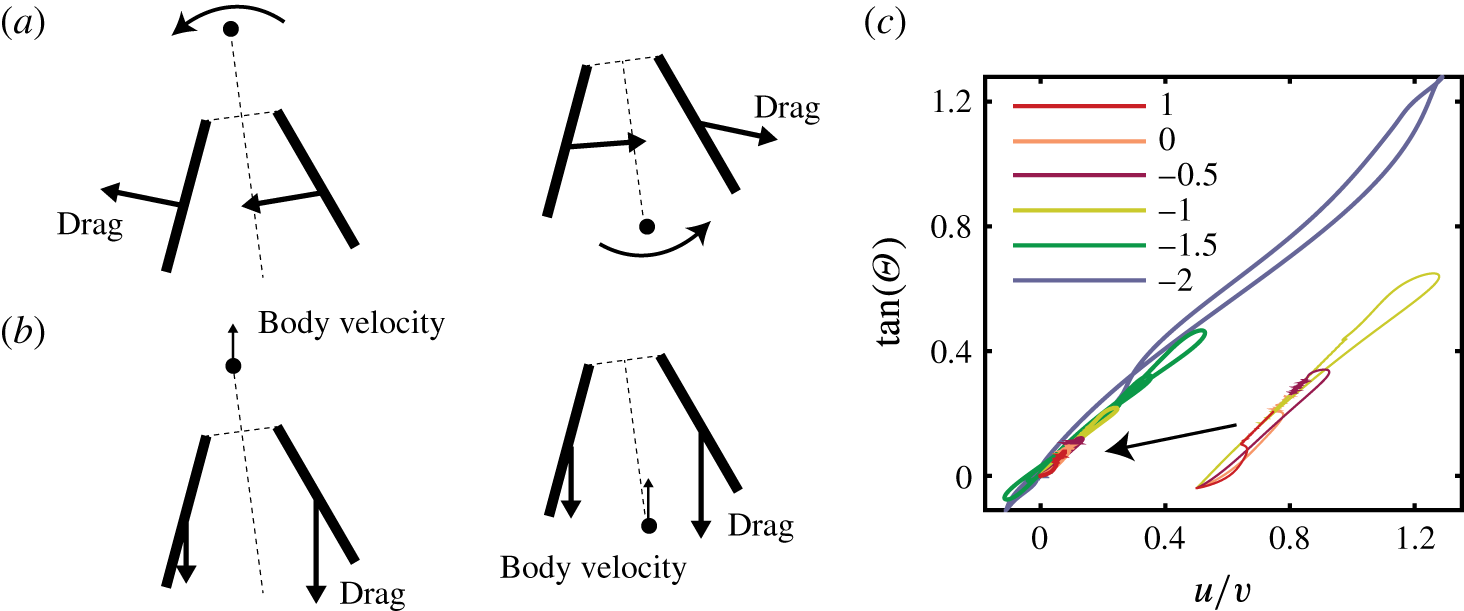
Stability mechanisms during ascent. (a) Schematics of the rotation-induced restoring torque. The sudden angular motion causes a motion of the wings, which induces a restoring torque on both the top-heavy flyers (left) and the bottom-heavy flyers (right). (b) Torque associated with misalignment of body orientation and body velocity. (c) Flyer’s orientation
 $\unicode[STIX]{x1D6E9}(t)$
is aligned with the flying velocity
 $(u(t),v(t)),~t\in [0,50]$
. Here the impulse strength is
 $\unicode[STIX]{x1D716}=100$
.

The stability of ascending flight, on the other hand, seems to be beyond what a simple linear model can capture. While we do not have a simple explanation for the stability characteristics during ascent, we can speculate about some contributing factors. First, we have identified a resistive torque that tends to immediately counteract the sudden rotation of the flyer during a perturbation. When the flyer tilts suddenly, it’s rotational motion is necessarily accompanied by a motion of the wings, as displayed in figure 13(a). The motion of the wings is associated with a drag in the opposite direction of the wing’s motion and thus induces a stabilizing torque that resists the external perturbation. This resistive torque can be seen in figure 10(c) for
 $t\in [13.3,13.7]$
. This rotation-induced torque is always a restoring torque for all the flyers. However, the torque is stronger on the top-heavy flyers and weaker on the bottom-heavy flyers, as the top-heavy flyers have longer torque arms. Secondly, we have identified an aerodynamic torque associated with the sudden change in the tilt angle, which results in a misalignment of the body orientation with the body velocity, as shown in figure 13(b). For top-heavy flyers in ascent, the increased drag on one wing relative to the other would seem to cause the body to align with its velocity. This is often called ‘weathercock stability’ (Watkins et al.
Reference Watkins, Milbank, Loxton and Melbourne2006) and is well known in the literature of airplanes and rockets (Etkin & Reid Reference Etkin and Reid1995). The case of bottom-heavy flyers is more subtle in this respect. As shown in the right panel of figure 13(b), whether the modified wing forces provide a resistive or amplifying torque would seem to depend on details of the changes in forces, the centre-of-mass location, and the degree of tilt of the body. In particular, it is not at all clear whether the line of action of the net force on the wings is to the left or right of the centre of mass.
Nonetheless, weathercocking – or the alignment of the body with the direction of travel – seems to be a general feature of both top- and bottom-heavy flyers during ascent. Figure 13(c) shows that
 $\tan (\unicode[STIX]{x1D6E9}(t))\approx u(t)/v(t)$
for all flyers, where
 $u(t)$
is the flyer’s instantaneous horizontal speed and
 $v(t)$
is the instantaneous vertical speed. This orientation–velocity alignment is also observed in the experiments (cf. figure 5 of Ristroph & Childress (Reference Ristroph and Childress2014)), and is reminiscent of the flight of passive bodies such as shuttlecocks, darts and arrows, as well as powered objects like rockets. However, the wings of our flyer not only play the role of stabilizing vanes but are also the thrust-producing surfaces, and their motions and associated vortical flow fields may affect the weathercocking effect. Further, while weathercocking is an important aspect of the flight dynamics, it does not seem to offer an explanation for the robust upright stability for bottom-heavy flyers during ascent.
Future engineering designs of practical jellyfish-like aerial vehicles could be guided by our computational studies, with flight manoeuvrability and stability being achieved through controlling the parameters of flapping amplitude
 $\unicode[STIX]{x1D703}_{a}$
, frequency
 $f$
, the wing separation
 $d$
and the centre-of-mass location
 $h$
. In our study, the hovering state and steady ascent state are found by tuning the flapping amplitude
 $\unicode[STIX]{x1D703}_{a}$
with the flapping frequency
 $f$
and wing separation
 $d$
fixed. One can also tune
 $f$
or
 $d$
and keep the other two fixed. Regarding engineering convenience, tuning frequency
 $f$
might be practically easier than tuning
 $\unicode[STIX]{x1D703}_{a}$
and
 $d$
. In future work, the relationship of the combination of these parameters and the resulting flight performance needs to be examined, and the effect on hovering of these parameters can be studied. For example, increasing
 $d$
(bringing wings further) could lead to a lift reduction and it might require increasing
 $\unicode[STIX]{x1D703}_{a}$
or
 $f$
to generate more lift to balance weight. The importance of the centre-of-mass location to flight stability has also been shown in our study, which suggests an approach to flight stability and control in which the centre of mass is dynamically changed during flight.
Acknowledgements
We thank N. Moore, S. Alben, L. Greengard, S. Childress and J. Zhang for fruitful discussions. This work was supported by the Lyttle Chair in Applied Mathematics. K.L.H. was partially supported by NSF award DMS-1203554.
Supplementary movies
Supplementary movies are available at https://doi.org/10.1017/jfm.2017.150.
Appendix A. Vortex sheet model
Using complex variables, at any point
 $z=x+\text{i}y$
, the conjugate of the flow velocity
 $u_{x}-\text{i}u_{y}$
(
 $\boldsymbol{u}=(u_{x},u_{y})$
in vector form) at any point
 $z$
not on the vortex sheet can be calculated through the Biot–Savart law by integrating the true vortex sheet strength
 $\hat{\unicode[STIX]{x1D6FE}}_{k}$
against the Biot–Savart kernel:
 $$\begin{eqnarray}\overline{w}(z)=u_{x}(z)-\text{i}u_{y}(z)=U+\frac{1}{2\unicode[STIX]{x03C0}\text{i}}\mathop{\sum }_{k=1,2}\int _{C_{k}^{b}+C_{k}^{f}}\frac{\hat{\unicode[STIX]{x1D6FE}}_{k}(s)}{z-\unicode[STIX]{x1D701}_{k}(s)}\,\text{d}s.\end{eqnarray}$$
Here
 $C_{k}^{b}:-1\leqslant s\leqslant 1$
denotes the contours of the bound vortex sheets (i.e. the wings, where
 $k=1,2$
), and
 $C_{k}^{f}:1\leqslant s\leqslant s_{max}^{k}$
denotes the contours of the two free vortex sheets attached to each wing, and
 $s$
is the arclength parameter. The location of the vortex sheet is denoted by
 $\unicode[STIX]{x1D701}_{k}$
. The first term
 $U$
in (A 1) denotes a prescribed dimensionless uniform background stream (see § 4.1). This velocity expression yields a continuous normal velocity and a jump in tangential velocity whose magnitude is given by
 $\hat{\unicode[STIX]{x1D6FE}}$
. The average
 $w_{k}(s,t)$
of the flow velocities on either side at points
 $\unicode[STIX]{x1D701}_{k}(s,t)$
on the vortex sheets is given by
 $$\begin{eqnarray}\displaystyle \overline{w}_{1}(\unicode[STIX]{x1D701}_{1}(s,t),t) & = & \displaystyle U(t)+\,\frac{1}{2\unicode[STIX]{x03C0}\text{i}}\quad \,P\!\!\!\!\!\!\!\int _{-1}^{s_{max}^{1}}\frac{\hat{\unicode[STIX]{x1D6FE}}_{1}(s^{\prime },t)\,\text{d}s^{\prime }}{\unicode[STIX]{x1D701}_{1}(s,t)-\unicode[STIX]{x1D701}_{1}(s^{\prime },t)}\nonumber\\ \displaystyle & & \displaystyle +\,\frac{1}{2\unicode[STIX]{x03C0}\text{i}}\int _{-1}^{s_{max}^{2}}\frac{\hat{\unicode[STIX]{x1D6FE}}_{2}(s^{\prime },t)\,\text{d}s^{\prime }}{\unicode[STIX]{x1D701}_{1}(s,t)-\unicode[STIX]{x1D701}_{2}(s^{\prime },t)},\end{eqnarray}$$
 $$\begin{eqnarray}\displaystyle \overline{w}_{2}(\unicode[STIX]{x1D701}_{2}(s,t),t) & = & \displaystyle U(t)+\,\frac{1}{2\unicode[STIX]{x03C0}\text{i}}\int _{-1}^{s_{max}^{1}}\frac{\hat{\unicode[STIX]{x1D6FE}}_{1}(s^{\prime },t)\,\text{d}s^{\prime }}{\unicode[STIX]{x1D701}_{2}(s,t)-\unicode[STIX]{x1D701}_{1}(s^{\prime },t)}\nonumber\\ \displaystyle & & \displaystyle +\,\frac{1}{2\unicode[STIX]{x03C0}\text{i}}\quad \,P\!\!\!\!\!\!\!\int _{-1}^{s_{max}^{2}}\frac{\hat{\unicode[STIX]{x1D6FE}}_{2}(s^{\prime },t)\,\text{d}s^{\prime }}{\unicode[STIX]{x1D701}_{2}(s,t)-\unicode[STIX]{x1D701}_{2}(s^{\prime },t)},\end{eqnarray}$$
where the bar denotes the complex conjugate and
 $\,P\!\!\!\int$
denotes the Cauchy principal value integral. Where convenient we shall simply use
 $\overline{w}_{k}(s,t)$
rather than
 $\overline{w}_{k}(\unicode[STIX]{x1D701}_{1}(s,t),t)$
.
The dynamics of the free sheet is most easily posed and evolved in the average velocity frame. Introducing
 $\unicode[STIX]{x1D6FC}$
a new parametrization of the sheet we have (Shelley Reference Shelley1992),
 $$\begin{eqnarray}\unicode[STIX]{x2202}_{t}\unicode[STIX]{x1D701}_{k}(\unicode[STIX]{x1D6FC},t)=w_{k}(\unicode[STIX]{x1D701}_{k}(\unicode[STIX]{x1D6FC},t),t).\end{eqnarray}$$
In that frame we have for the unnormalized vortex sheet strength the conservation law:
 $$\begin{eqnarray}\unicode[STIX]{x2202}_{t}\unicode[STIX]{x1D6FE}_{k}(\unicode[STIX]{x1D6FC},t)=0.\end{eqnarray}$$
We will refer to the average velocity frame of the free sheet as the Lagrangian frame (since circulation is conserved in that frame), and to
 $\unicode[STIX]{x1D6FC}$
as the Lagrangian variable or marker. For convenience we retain the
 $s$
parametrization of the free sheet velocity integrals in (A 2)–(A 3), and trivially evolve the
 $s$
parametrization in the average velocity frame; see below.
On the bound vortex sheets,
 $C_{k}^{b}$
, the arclength
 $s$
is a material variable for the wings (seen as rigid plates). The flyer’s location is determined by the flyer’s body variables
 $(Z(t),\unicode[STIX]{x1D6E9}(t))$
, where
 $Z(t)$
denotes the location of the flyer’s centre of mass in the complex form. The location of any point on the rigid wing (
 $-1\leqslant s\leqslant 1$
) can be expressed as
 $$\begin{eqnarray}\displaystyle & \displaystyle \unicode[STIX]{x1D701}_{k}(s,t)=(s+1){\hat{s}}_{k}+\unicode[STIX]{x1D701}_{k}(-1,t), & \displaystyle\end{eqnarray}$$
 $$\begin{eqnarray}\displaystyle & \displaystyle \unicode[STIX]{x1D701}_{k}(-1,t)=Z(t)-h\exp \left(\text{i}\left(\frac{\unicode[STIX]{x03C0}}{2}-\unicode[STIX]{x1D6E9}(t)\right)\right)\pm \frac{d}{2}\text{e}^{\text{i}\unicode[STIX]{x1D6E9}(t)}. & \displaystyle\end{eqnarray}$$
Here
 $\unicode[STIX]{x1D701}_{k}(-1,t)$
is the location of the wing’s leading edge or hinge (see figure 1
c), and
 $$\begin{eqnarray}{\hat{s}}_{k}(t)=\exp \left(\text{i}\left(\unicode[STIX]{x1D703}_{k}(t)+\unicode[STIX]{x1D6E9}(t)-\frac{\unicode[STIX]{x03C0}}{2}\right)\right)\end{eqnarray}$$
is the complex form of the tangent vector to the bound sheet (see (2.1)). The normal vector is then
 $$\begin{eqnarray}\hat{n}_{k}(t)=\text{i}{\hat{s}}_{k}(t)=\text{e}^{\text{i}(\unicode[STIX]{x1D703}_{k}(t)+\unicode[STIX]{x1D6E9}(t))}.\end{eqnarray}$$
The no-penetration boundary condition, equation (2.6), yields on the bound vortex sheet:
 $$\begin{eqnarray}\text{Re}\left(\hat{n}_{k}\left(\unicode[STIX]{x2202}_{t}\overline{\unicode[STIX]{x1D701}}_{k}(s,t)-\overline{w}_{k}(s,t)\right)\right)=0,\quad -1\leqslant s\leqslant 1.\end{eqnarray}$$
Substituting (A 2)–(A 3) and (A 6)–(A 9) into (A 10a,b
), we see that (A 10a,b
) is an integral equation for the vortex sheet strength
 $\hat{\unicode[STIX]{x1D6FE}}_{k}(s,t),\;-1\leqslant s\leqslant 1$
, which requires one more constraint to determine an integration constant. This constraint is provided by applying the Kelvin’s circulation theorem on each wing and the free vortex sheet attached to it, which states that the total circulation of each wing and its free vortex sheet is conserved, i.e.
 $$\begin{eqnarray}C=\int _{-1}^{s_{max}^{k}}\hat{\unicode[STIX]{x1D6FE}}_{k}(s,t)\,\text{d}s=\int _{-1}^{1}\hat{\unicode[STIX]{x1D6FE}}_{k}(s,0)\,\text{d}s.\end{eqnarray}$$
We start with
 $\hat{\unicode[STIX]{x1D6FE}}_{k}(s,0)=0$
at
 $t=0$
, giving
 $C=0$
, with the free vortex sheet is initially a single point at the wing trailing edge, i.e.
 $s_{max}^{k}|_{t=0}=1$
. Denoting the total circulation around the wing by
 $\unicode[STIX]{x1D6E4}_{k}(t)=\int _{-1}^{1}\hat{\unicode[STIX]{x1D6FE}}_{k}(s,t)\,\text{d}s$
, we then have
 $$\begin{eqnarray}\unicode[STIX]{x1D6E4}_{k}(t)=-\int _{1}^{s_{max}^{k}}\hat{\unicode[STIX]{x1D6FE}}_{k}(s,t)\,\text{d}s.\end{eqnarray}$$
The unsteady Kutta condition applied at the wing’s trailing edge determines the rate of vorticity shedding (see Jones Reference Jones2003), as
 $$\begin{eqnarray}\dot{\unicode[STIX]{x1D6E4}}_{k}(t)+(\unicode[STIX]{x1D707}_{k}(1,t)-\unicode[STIX]{x1D709}_{k}(1,t))\hat{\unicode[STIX]{x1D6FE}}_{k}(1,t)=0,\end{eqnarray}$$
where
 $\unicode[STIX]{x1D709}_{k}(s,t)=\text{Re}({\hat{s}}_{k}\unicode[STIX]{x2202}_{t}\overline{\unicode[STIX]{x1D701}}_{k}(s,t))$
is the tangential component of the wing velocity and
 $\unicode[STIX]{x1D707}_{k}(s,t)=\text{Re}({\hat{s}}_{k}\overline{w}_{k}(s,t))$
is the tangential component of the average fluid velocity at the wing boundary. The fluid and the wings are related through the pressure force on the wings (2.7)–(2.8). On the bound vortex sheet the pressure jump and vorticity satisfy the following variation of the Euler equations (Jones Reference Jones2003; Alben Reference Alben2009)
 $$\begin{eqnarray}\unicode[STIX]{x2202}_{t}\hat{\unicode[STIX]{x1D6FE}}_{k}+\unicode[STIX]{x2202}_{s}((\unicode[STIX]{x1D707}_{k}-\unicode[STIX]{x1D709}_{k})\hat{\unicode[STIX]{x1D6FE}}_{k})=\unicode[STIX]{x2202}_{s}[p_{k}],\quad -1\leqslant s\leqslant 1,\end{eqnarray}$$
found by posing the Euler equations, above and below the bound sheet, in the common
 $s$
-frame, and taking their tangential difference (How, Lowengrub & Shelley Reference How, Lowengrub and Shelley1994). The boundary condition to (A 14) is that the pressure is continuous at the wing’s trailing edge where
 $s=1$
:
 $$\begin{eqnarray}[p_{k}](1,t)=0.\end{eqnarray}$$
Integrating equation (A 14), using the boundary condition equation (A 15) and the Kutta condition equation (A 13), the pressure jump distribution on the wing is then
 $$\begin{eqnarray}[p_{k}](s,t)=\int _{1}^{s}\unicode[STIX]{x2202}_{t}\hat{\unicode[STIX]{x1D6FE}}_{k}(s^{\prime },t)\,\text{d}s^{\prime }+(\unicode[STIX]{x1D707}_{k}(s,t)-\unicode[STIX]{x1D709}_{k}(s,t))\hat{\unicode[STIX]{x1D6FE}}_{k}(s,t)+\dot{\unicode[STIX]{x1D6E4}}_{k}(t).\end{eqnarray}$$
We summarize the unknowns and the equations as follows:
-
(i) The flyer’s dynamical variables, the centre-of-mass location
 $\boldsymbol{X}(t)$
and tilt angle
$\unicode[STIX]{x1D6E9}(t)$
, are governed by (2.7)–(2.8), given in the real form, where the fluid pressure force is provided by (A 16);
-
(ii) The free vortex sheets’ location
$\unicode[STIX]{x1D701}_{k}(s,t)$
and the free vortex sheet strengths
$\hat{\unicode[STIX]{x1D6FE}}_{k}(s,t)$
are given by (A 4)–(A 5), where
$1\leqslant s\leqslant s_{max}^{k}$
; -
(iii) The bound vortex sheet strength
$\hat{\unicode[STIX]{x1D6FE}}_{k}(s,t),~-1\leqslant s\leqslant 1$
and the circulation around the wing
$\unicode[STIX]{x1D6E4}_{k}(t)$
are found by the kinematic boundary condition equation (A 10a,b
), the circulation theorem equation (A 11) and the Kutta condition of the vortex shedding equation (A 13).




Appendix B. Numerical method
B.1 Explicit method for the free vortex sheet
The free vortex sheet is discretized and evolved in the average velocity frame. At each time step, a vortex sheet segment is shed into the existing free sheet at the wing trailing edge, and then convects with velocity given by (A 4). At time
 $t_{n}$
, we denote
 $[\unicode[STIX]{x1D701}_{f,k}^{j-1,n},\unicode[STIX]{x1D701}_{f,k}^{j,n}]$
the segment shed at time
 $t_{j}$
, for
 $1\leqslant j\leqslant n$
(no segment shed at
 $t_{0}$
). Note that
 $\unicode[STIX]{x1D701}_{f,k}^{j,n}$
,
 $0\leqslant j\leqslant n$
, are Lagrangian points, and
 $\unicode[STIX]{x1D701}_{f,k}^{n,n}$
is the newly generated endpoint of the free sheet which is also the wing’s trailing edge.
The updating for the free vortex sheet position goes as follows. The endpoints of segments generated at and before time
 $t_{n-1}$
are updated explicitly by a second-order Adam–Bashforth method, and the endpoint
 $\unicode[STIX]{x1D701}_{f,k}^{n,n}$
of the last segment created at
 $t_{n}$
is updated using the Euler method:
 $$\begin{eqnarray}\displaystyle & \displaystyle \unicode[STIX]{x1D701}_{f,k}^{j,n+1}=\unicode[STIX]{x1D701}_{f,k}^{j,n}+\frac{\unicode[STIX]{x0394}t}{2}\left(3w_{k}(\unicode[STIX]{x1D701}_{f,k}^{j,n})-w_{k}(\unicode[STIX]{x1D701}_{f,k}^{j,n-1})\right),\quad j=0,\ldots ,n-1 & \displaystyle\end{eqnarray}$$
 $$\begin{eqnarray}\displaystyle & \displaystyle \unicode[STIX]{x1D701}_{f,k}^{n,n+1}=\unicode[STIX]{x1D701}_{f,k}^{n,n}+\unicode[STIX]{x0394}t\,w_{k}(\unicode[STIX]{x1D701}_{f,k}^{n,n}). & \displaystyle\end{eqnarray}$$
To evaluate the boundary integral in (A 4) for the free sheet velocity we use Chebyshev quadrature (Mason & Handscomb Reference Mason and Handscomb2002) on the bound sheets and the trapezoidal rule on the free sheets.
We define
 $\hat{\unicode[STIX]{x1D6FE}}_{f,k}^{j,n}$
as the mean of the true vortex sheet strength over the sheet segment
 $[\unicode[STIX]{x1D701}_{f,k}^{j-1,n},\unicode[STIX]{x1D701}_{f,k}^{j,n}]$
, i.e.
 $$\begin{eqnarray}\hat{\unicode[STIX]{x1D6FE}}_{f,k}^{j,n}=\int _{s_{j}^{n}}^{s_{j-1}^{n}}\hat{\unicode[STIX]{x1D6FE}}_{k}(s^{\prime })\,\text{d}s^{\prime }/(s_{j-1}^{n}-s_{j}^{n}),\end{eqnarray}$$
where
 $s_{j}^{n},0\leqslant j\leqslant n$
, denotes the arclength at point
 $\unicode[STIX]{x1D701}_{f,k}^{j,n}$
,
 $s_{0}^{n}=s_{max}$
corresponds to the endpoint
 $\unicode[STIX]{x1D701}_{f,k}^{0,n}$
, and
 $s_{n}^{n}=1$
corresponds to the wing trailing edge. As the unnormalized vortex sheet strength
 $\unicode[STIX]{x1D6FE}$
is a material quantity (A 5), the circulation on the segment
 $\int _{\unicode[STIX]{x1D6FC}_{j+1}}^{\unicode[STIX]{x1D6FC}_{j}}\unicode[STIX]{x1D6FE}_{k}(\unicode[STIX]{x1D6FC}^{\prime })\,\text{d}\unicode[STIX]{x1D6FC}^{\prime }=\int _{s_{j+1}^{n}}^{s_{j}^{n}}\hat{\unicode[STIX]{x1D6FE}}_{k}(s^{\prime })\,\text{d}s^{\prime }$
does not change with time, therefore at
 $t_{n+1}$
the vortex sheet strength is updated as
 $$\begin{eqnarray}\hat{\unicode[STIX]{x1D6FE}}_{f,k}^{j,n+1}=\hat{\unicode[STIX]{x1D6FE}}_{f,k}^{j,n}(s_{j-1}^{n}-s_{j}^{n})/(s_{j-1}^{n+1}-s_{j}^{n+1}),\quad j=1,\ldots ,n.\end{eqnarray}$$
The circulation on the newly generated segment
 $[\unicode[STIX]{x1D701}_{f,k}^{n,n+1},\unicode[STIX]{x1D701}_{f,k}^{n+1,n+1}]$
equals the opposite of the circulation change of the wing (A 12). The mean vortex sheet strength on the last vortex sheet segment is thus given as:
 $$\begin{eqnarray}\hat{\unicode[STIX]{x1D6FE}}_{f,k}^{n+1,n+1}=-(\unicode[STIX]{x1D6E4}_{k}^{n+1}-\unicode[STIX]{x1D6E4}_{k}^{n})/(s_{n}^{n+1}-1),\end{eqnarray}$$
where
 $\unicode[STIX]{x1D6E4}_{k}^{n}=\unicode[STIX]{x1D6E4}_{k}(t_{n}),k=1,2$
denotes the wing circulation at time
 $t_{n}$
. The last segment’s mean vortex sheet strength
 $\hat{\unicode[STIX]{x1D6FE}}_{f,k}^{n+1,n+1}$
and its endpoint
 $\unicode[STIX]{x1D701}_{f,k}^{n+1,n+1}$
(located at the wing trailing edge) are computed in the implicit step next, where the updated wing circulation
 $\unicode[STIX]{x1D6E4}_{k}^{n+1}$
and wing trailing-edge position are determined.
B.2 Implicit method for the body
When the free vortex sheets are updated to
 $(\unicode[STIX]{x1D701}_{f,k}^{j,n+1},\hat{\unicode[STIX]{x1D6FE}}_{f,k}^{j,n+1}),j=1,\ldots ,n$
, the bound vortex sheets’ locations and strengths need to be updated to match the new free sheets. There are three equations to be solved implicitly, the boundary integral equation (A 10a,b
), and the flyer’s dynamics equations, (2.7) and (2.8).
The no-penetration condition on the wing (A 10a,b ) can be simplified, using expressions (A 2)–(A 3) and (A 6)–(A 7), to
 $$\begin{eqnarray}\frac{1}{2\unicode[STIX]{x03C0}}\quad \,P\!\!\!\!\!\!\!\int _{-1}^{1}\frac{\hat{\unicode[STIX]{x1D6FE}}_{k}(s^{\prime },t)}{s-s^{\prime }}\,\text{d}s^{\prime }=f_{k}(s,t)-\frac{1}{2\unicode[STIX]{x03C0}}\hat{\unicode[STIX]{x1D6FE}}_{k}(1,t)\ln (1-s),\end{eqnarray}$$
where
 $$\begin{eqnarray}\displaystyle f_{k}(s,t) & = & \displaystyle \text{Re}\left[\hat{n}_{k}\left(-U(t)+\unicode[STIX]{x2202}_{t}\overline{\unicode[STIX]{x1D701}}_{k}(s,t)-\frac{1}{2\unicode[STIX]{x03C0}\text{i}}\int _{1}^{s_{max}^{k}}\frac{\hat{\unicode[STIX]{x1D6FE}}_{k}(s^{\prime },t)}{\unicode[STIX]{x1D701}_{k}(s,t)-\unicode[STIX]{x1D701}_{k}(s^{\prime },t)}\,\text{d}s^{\prime }\right.\right.\nonumber\\ \displaystyle & & \displaystyle \left.\left.-\frac{1}{2\unicode[STIX]{x03C0}\text{i}}\int _{-1}^{s_{max}^{l}}\frac{\hat{\unicode[STIX]{x1D6FE}}_{l}(s^{\prime },t)}{\unicode[STIX]{x1D701}_{k}(s,t)-\unicode[STIX]{x1D701}_{l}(s^{\prime },t)}\,\text{d}s^{\prime }\right)\right]+\frac{1}{2\unicode[STIX]{x03C0}}\hat{\unicode[STIX]{x1D6FE}}_{k}(1,t)\ln (1-s),\quad l\neq k,\quad\end{eqnarray}$$
is a continuous function in
 $s\in [-1,1]$
, with a logarithmic singularity explicitly subtracted (Alben Reference Alben2010). Equation (B 6) is an integral equation, and its solution
 $\hat{\unicode[STIX]{x1D6FE}}_{k}(s,t)$
contains an inverse-square-root singularity at the wing’s leading edge,
 $s=-1$
(Golberg Reference Golberg2013). Therefore we define
 $\unicode[STIX]{x1D708}_{k}(s,t)=\hat{\unicode[STIX]{x1D6FE}}_{k}(s,t)\sqrt{1-s^{2}}$
and solve for
 $\unicode[STIX]{x1D708}_{k}(s,t)$
and the wing circulation
 $\unicode[STIX]{x1D6E4}_{k}(t)$
, instead of solving for
 $\hat{\unicode[STIX]{x1D6FE}}_{k}$
and
 $\unicode[STIX]{x1D6E4}_{k}$
.
We discretize the wing (the bound sheet
 $C_{k}^{b}:-1\leqslant s\leqslant 1$
) using
 $m+1$
Chebyshev–Gauss–Lobatto nodes
 $$\begin{eqnarray}s_{i}=\cos (\unicode[STIX]{x1D719}_{i}),\quad \unicode[STIX]{x1D719}_{i}=\frac{i\unicode[STIX]{x03C0}}{m},\quad i=0,\ldots ,m,\end{eqnarray}$$
interpolate
 $f_{k}(s,t)$
at
 $s_{i}$
by the
 $m\text{th}$
-order polynomial and then expand in a Chebyshev series:
 $$\begin{eqnarray}f_{k}(s,t)=\mathop{\sum }_{j=0}^{m}a_{k}^{j}(t)\cos (j\unicode[STIX]{x1D719}),\quad \text{where }s=\cos (\unicode[STIX]{x1D719}).\end{eqnarray}$$
The solution to (B 6) is given as (Golberg Reference Golberg2013)
 $$\begin{eqnarray}\displaystyle \unicode[STIX]{x1D708}_{k}(s,t) & = & \displaystyle 2\mathop{\sum }_{j=1}^{m}a_{k}^{j}(t)\sin (\unicode[STIX]{x1D719}(s))\sin (j\unicode[STIX]{x1D719}(s))-a_{k}^{1}(t)-2a_{k}^{0}(t)s+\frac{\unicode[STIX]{x1D6E4}_{k}(t)}{\unicode[STIX]{x03C0}}\nonumber\\ \displaystyle & & \displaystyle +\,\frac{\hat{\unicode[STIX]{x1D6FE}}_{k}(1,t)}{\unicode[STIX]{x03C0}}\sqrt{1-s^{2}}(\unicode[STIX]{x03C0}-\unicode[STIX]{x1D719}(s))-\frac{\hat{\unicode[STIX]{x1D6FE}}_{k}(1,t)}{\unicode[STIX]{x03C0}}(1+s\ln 2).\end{eqnarray}$$
The constant in the integration is determined by the definition of
 $\unicode[STIX]{x1D6E4}_{k}(t)=\int _{-1}^{1}\hat{\unicode[STIX]{x1D6FE}}_{k}(s,t)\,\text{d}s$
. The Kutta condition, equation (A 13), which implies that the trailing-edge vorticity
 $\hat{\unicode[STIX]{x1D6FE}}_{k}(1,t)$
is finite, enforces another constraint:
 $$\begin{eqnarray}\unicode[STIX]{x1D708}_{k}(1,t)=-a_{k}^{1}(t)-2a_{k}^{0}(t)+\frac{\unicode[STIX]{x1D6E4}_{k}(t)}{\unicode[STIX]{x03C0}}-\frac{\hat{\unicode[STIX]{x1D6FE}}_{k}(1,t)}{\unicode[STIX]{x03C0}}(1+\ln 2)=0.\end{eqnarray}$$
Denote
 $\unicode[STIX]{x1D708}_{k}^{i,n}=\unicode[STIX]{x1D708}_{k}(s_{i},t_{n}),~i=0,\ldots ,m$
and
 $\unicode[STIX]{x1D6E4}_{k}^{n}=\unicode[STIX]{x1D6E4}_{k}(t_{n})$
. To solve at time
 $t_{n+1}$
, equations (B 10)–(B 11), discretized at Chebyshev–Gauss–Lobatto nodes, are given as
 $$\begin{eqnarray}\displaystyle 0 & = & \displaystyle \unicode[STIX]{x1D708}_{k}^{i,n+1}-2\mathop{\sum }_{j=1}^{m}a_{k}^{j,n+1}\sin (\unicode[STIX]{x1D719}_{i})\sin (j\unicode[STIX]{x1D719}_{i})+a_{k}^{1,n+1}+2a_{k}^{0,n+1}s_{i}-\frac{\unicode[STIX]{x1D6E4}_{k}^{n+1}}{\unicode[STIX]{x03C0}}\nonumber\\ \displaystyle & & \displaystyle -\,\frac{\hat{\unicode[STIX]{x1D6FE}}_{k}^{0,n+1}}{\unicode[STIX]{x03C0}}\sqrt{1-s_{i}^{2}}(\unicode[STIX]{x03C0}-\unicode[STIX]{x1D719}_{i})+\frac{\hat{\unicode[STIX]{x1D6FE}}_{k}^{0,n+1}}{\unicode[STIX]{x03C0}}(1+s_{i}\ln 2),~i=1,\ldots ,m,\end{eqnarray}$$
 $$\begin{eqnarray}\displaystyle 0 & = & \displaystyle 2a_{k}^{0,n+1}-\frac{\unicode[STIX]{x1D6E4}_{k}^{n+1}}{\unicode[STIX]{x03C0}}+\frac{\hat{\unicode[STIX]{x1D6FE}}_{k}^{0,n+1}}{\unicode[STIX]{x03C0}}(1+\ln 2),\end{eqnarray}$$
where
 $s_{i}=\cos (\unicode[STIX]{x1D719}_{i}),~a_{k}^{j,n+1}=a_{k}^{j}(t_{n+1}),~i,j=0,\ldots ,m$
and
 $\hat{\unicode[STIX]{x1D6FE}}_{k}^{0,n+1}=\hat{\unicode[STIX]{x1D6FE}}_{k}(1,t_{n+1})$
. Note that
 $\hat{\unicode[STIX]{x1D6FE}}_{k}^{0,n+1}$
also equals
 $\hat{\unicode[STIX]{x1D6FE}}_{f,k}^{n+1,n+1}$
as the vortex sheet strength is continuous at the wing trailing edge (see (B 5)).
The flyer’s dynamics equations, (2.7)–(2.8), are also implicitly discretized, and coupled with (B 12)–(B 13), since the bound vortex sheets positions’ are determined by the dynamical variables
 $\boldsymbol{X}$
and
 $\unicode[STIX]{x1D6E9}$
through (2.1) and (A 6)–(A 8). Defining
 $\boldsymbol{X}^{n+1}=\boldsymbol{X}(t_{n+1}),~\dot{\boldsymbol{X}}^{n+1}=\dot{\boldsymbol{X}}(t_{n+1})$
,
 $\unicode[STIX]{x1D6E9}^{n+1}=\unicode[STIX]{x1D6E9}(t_{n+1}),~\dot{\unicode[STIX]{x1D6E9}}^{n+1}=\dot{\unicode[STIX]{x1D6E9}}(t_{n+1})$
, we use the second-order Crank–Nicolson time stepping for the flyer’s dynamics:
 $$\begin{eqnarray}0=\boldsymbol{X}^{n+1}-\boldsymbol{X}^{n}-\frac{\unicode[STIX]{x0394}t}{2}(\dot{\boldsymbol{X}}^{n+1}+\dot{\boldsymbol{X}}^{n}),\quad 0=\dot{\boldsymbol{X}}^{n+1}-\dot{\boldsymbol{X}}^{n}-\frac{\unicode[STIX]{x0394}t}{2M}({\mathcal{F}}^{n+1}+{\mathcal{F}}^{n}),\end{eqnarray}$$
 $$\begin{eqnarray}0=\unicode[STIX]{x1D6E9}^{n+1}-\unicode[STIX]{x1D6E9}^{n}-\frac{\unicode[STIX]{x0394}t}{2}(\dot{\unicode[STIX]{x1D6E9}}^{n+1}+\dot{\unicode[STIX]{x1D6E9}}^{n}),\quad 0=\dot{\unicode[STIX]{x1D6E9}}^{n+1}-\dot{\unicode[STIX]{x1D6E9}}^{n}-\frac{\unicode[STIX]{x0394}t}{2I}({\mathcal{T}}^{n+1}+{\mathcal{T}}^{n}),\end{eqnarray}$$
where
 ${\mathcal{F}}^{n}={\mathcal{F}}(t_{n})$
denotes the net force on the flyer at
 $t_{n}$
and
 ${\mathcal{T}}^{n}={\mathcal{T}}(t_{n})$
denotes the torque (see (2.7)–(2.8)), and they are evaluated by integrating the fluid pressure along the wing (A 16).
To summarize, at the step from
 $t_{n}$
to
 $t_{n+1}$
, the implicit system consists of
 $2(m+1)+4$
equations (B 12)–(B 14), while there are
 $2(m+1)+4$
unknowns:
 $\unicode[STIX]{x1D708}_{k}^{i,n+1},~i=1,\ldots ,m$
,
 $\unicode[STIX]{x1D6E4}_{k}^{n+1},~k=1,2$
and
 $\boldsymbol{X}^{n+1}=\boldsymbol{X}(t_{n+1}),~\dot{\boldsymbol{X}}^{n+1}$
,
 $\unicode[STIX]{x1D6E9}^{n+1},~\dot{\unicode[STIX]{x1D6E9}}^{n+1}$
. In our numerical method, Chebyshev quadrature is applied to the integrals over the bound sheets, as in (2.7)–(2.8), (A 16–2.11) and (B 7). The time derivatives in (A 16) and (B 7) are treated using second-order Richardson extrapolation. This nonlinear system is solved by the Broyden’s method (Broyden Reference Broyden1965). It is a quasi-Newton method that each iteration requires
 $O(N^{2})$
operations, where
 $N=2m+6$
is the system size. The convergence of a quasi-Newton method is in general superlinear, which is slightly slower than Newton’s method but is of low cost. In our case, with a error tolerance set at
 $10^{-10}$
, the algorithm converges in approximately
 $10{-}20$
iterations.
B.3 Velocity
$\unicode[STIX]{x1D6FF}-$
smoothing treatment

The Birkhoff–Rott equation (A 2)–(A 4) for the dynamics of free vortex sheets is mathematically ill posed, and it is well known that it leads to a curvature singularity in finite time, before the rolling up of the sheets (Moore Reference Moore1979; Krasny Reference Krasny1986; Shelley Reference Shelley1992). To subvert both the ill posedness and the singularity, and allow the sheets to form vortex spirals, we regularize the singular kernel in (A 1) using the Krasny
 $\unicode[STIX]{x1D6FF}-$
smoothing method (Krasny Reference Krasny1986; Alben Reference Alben2009),
 $$\begin{eqnarray}\displaystyle \unicode[STIX]{x2202}_{t}\overline{\unicode[STIX]{x1D701}}_{k}(s,t) & = & \displaystyle U(t)+\frac{1}{2\unicode[STIX]{x03C0}\text{i}}\quad \,P\!\!\!\!\!\!\!\int _{-1}^{s_{max}^{k^{\prime }}}\frac{\hat{\unicode[STIX]{x1D6FE}}_{k^{\prime }}(s^{\prime },t)\,\text{d}s^{\prime }}{\unicode[STIX]{x1D701}_{k^{\prime }}(s,t)-\unicode[STIX]{x1D701}_{k^{\prime }}(s^{\prime },t)}\nonumber\\ \displaystyle & & \displaystyle +\,\frac{1}{2\unicode[STIX]{x03C0}\text{i}}\int _{-1}^{s_{max}^{k}}\hat{\unicode[STIX]{x1D6FE}}_{k}(s^{\prime },t)\,\text{d}s^{\prime }\frac{\overline{\unicode[STIX]{x1D701}}_{k}(s,t)-\overline{\unicode[STIX]{x1D701}}_{k}(s^{\prime },t)}{|\unicode[STIX]{x1D701}_{k}(s,t)-\unicode[STIX]{x1D701}_{k}(s^{\prime },t)|^{2}+\unicode[STIX]{x1D6FF}^{2}(s)}.\end{eqnarray}$$
The
 $\unicode[STIX]{x1D6FF}$
-smoothing is needed only on the dynamics of the free sheets, and we retain the singular structure for the bound sheet dynamics. To resolve the discontinuity in the velocity at the boundary between the bound sheet and the free sheet, i.e. the wing’s trailing edge, we use the velocity smoothing treatment of Alben (Reference Alben2010). The smoothing function we use in (B 16) is defined as:
 $$\begin{eqnarray}\displaystyle \unicode[STIX]{x1D6FF}(s) & = & \displaystyle \unicode[STIX]{x1D6FF}_{1}+(\unicode[STIX]{x1D6FF}_{0}-\unicode[STIX]{x1D6FF}_{1})\frac{|(s-1)/\unicode[STIX]{x1D702}_{1}|^{p}}{1+|(s-1)/\unicode[STIX]{x1D702}_{1}|^{p}},\quad s\in (\!1,s_{max}\! ]\end{eqnarray}$$
 $$\begin{eqnarray}\displaystyle \unicode[STIX]{x1D6FF}(s) & = & \displaystyle \unicode[STIX]{x1D6FF}_{1}\exp (-|(s-1)/\unicode[STIX]{x1D702}_{2}|^{p}),\quad s\in [-1,1].\end{eqnarray}$$
In our simulations, we set
 $\unicode[STIX]{x1D6FF}_{0}=0.2,~\unicode[STIX]{x1D6FF}_{1}=0.1,~\unicode[STIX]{x1D702}_{1}=2\unicode[STIX]{x1D6FF}_{0},~\unicode[STIX]{x1D702}_{2}=0.1$
and
 $p=2$
.
Appendix C. FMM for the regularized kernel
We assume that the kernel that we are interested in applying is
 $$\begin{eqnarray}\displaystyle K(z,z_{0})=-\frac{1}{2\unicode[STIX]{x03C0}N}\frac{\overline{z-z_{0}}}{|z-z_{0}|^{2}+\unicode[STIX]{x1D6FF}_{f}(z_{0})}, & & \displaystyle\end{eqnarray}$$
where
 $z,z_{0}\in \mathbb{C}$
are ‘complexified’ target and source points, respectively, in
 $\mathbb{R}^{2}$
(i.e. a point
 $(x,y)$
is mapped to the complex number
 $z=x+\text{i}y$
), and
 $\unicode[STIX]{x1D6FF}_{f}>0$
is a regularization term that we have access to only numerically. This kernel comes from considering the gradient of the two-dimensional Laplace potential, identified with the complex logarithm; thus, applying
 $K$
is, in effect, a force calculation.
Force calculations were accelerated using an adaptive kernel-independent FMM based on interpolative decomposition (ID) (Carrier, Greengard & Rokhlin Reference Carrier, Greengard and Rokhlin1988). The principal ideas have already appeared in Carrier et al. (Reference Carrier, Greengard and Rokhlin1988), Martinsson & Rokhlin (Reference Martinsson and Rokhlin2007), Pan & Sheng (Reference Pan and Sheng2013). In this section, we give a brief overview of the algorithm and highlight the specific modifications necessary to efficiently approximate the kernel (C 1) to high precision.
C.1 Overview of the FMM
Let
 $\unicode[STIX]{x1D63C}=(a_{ij})\in \mathbb{C}^{N\times N}$
with entries
 $a_{ij}=K(z_{i},z_{j})$
, where
 $K$
is a kernel function defined on the complex points
 $z_{i}\in \mathbb{C}$
for
 $i=1,\ldots ,N$
. We are interested in computing the matrix–vector product
 $\boldsymbol{x}\mapsto \unicode[STIX]{x1D63C}x$
, where
 $\boldsymbol{x}\in \mathbb{C}^{N}$
. If
 $\unicode[STIX]{x1D63C}$
is dense (as it is for the kernel (C 1)), then this operation naively requires
 $O(N^{2})$
work, which can be prohibitive if
 $N$
is large. The goal of the FMM is to reduce this to only
 $O(N)$
or
 $O(N\log N)$
work.
The main observation underlying the FMM is that for many choices of
 $K$
in practice,
 $\unicode[STIX]{x1D63C}$
contains large submatrices that are numerically low rank and so can be applied very efficiently; see figure 14(a). In essence, the FMM is simply a way of organizing such low-rank computations in order to achieve linear complexity.
(a) Rank structure of an FMM-compatible matrix in one dimension. Submatrices in white are low rank; those in grey are, in general, full rank. (b) Well-separated point clusters in the plane. (c) Definition of neighbours and interaction lists. The neighbours of a box
 $B$
are indicated in dark grey, while its interaction list is indicated in light grey; for reference, the parent of
 $B$
is drawn in a thick outline.

The core assumption in the FMM is that rank structure is determined by geometry. Two point clusters
 $C=\{x_{1},\ldots ,x_{m}\}$
and
 $C^{\prime }=\{y_{1},\ldots ,y_{n}\}$
in
 $\mathbb{C}$
are said to be well separated if
 $$\begin{eqnarray}\displaystyle \operatorname{dist}(C,C^{\prime })>\max (\operatorname{diam}(C),\operatorname{diam}(C^{\prime })), & & \displaystyle\end{eqnarray}$$
where
 $$\begin{eqnarray}\operatorname{dist}(C,C^{\prime })=\min _{\substack{ x\in C \\ y\in C^{\prime }}}|x-y|,\quad \operatorname{diam}(C)=\max _{x,y\in C}|x-y|;\end{eqnarray}$$
see figure 14(b). It is well known that for the kernel (C 1) with
 $\unicode[STIX]{x1D6FF}_{f}\equiv 0$
, interactions between well-separated sets have constant rank (to a specified numerical precision), independent of the number of points in each set or their detailed structure (Greengard & Rokhlin Reference Greengard and Rokhlin1987). We observed experimentally that the same appears to be true of the regularized kernel in this paper.
The remainder of the FMM consists of hierarchically decomposing
 $\unicode[STIX]{x1D63C}$
into well-separated interactions. This is done by constructing a quadtree on
 $\mathbb{C}$
. First, enclose all points inside a sufficiently large box. If the number of points in that box exceeds a prescribed constant, subdivide it into four equally sized children and split its points accordingly between them, keeping only those children that are non-empty. Repeat this procedure for each new box added, terminating only when all boxes contain only
 $O(1)$
points. Boxes that do not have any children are called leaves.
For simplicity, we assume that all leaves are at the same level in the tree. This makes the ensuing discussion much more concise while retaining the key features of the algorithm. For details regarding the fully adaptive version, which we implemented for this paper, we refer the reader to Carrier et al. (Reference Carrier, Greengard and Rokhlin1988), Martinsson & Rokhlin (Reference Martinsson and Rokhlin2007).
For each box
 $B$
in the tree, let its neighbours be those boxes at the same level immediately adjacent to it. Moreover, let its interaction list consist of those boxes at the same level whose parents are neighbours of the parent of
 $B$
but who are not themselves neighbours of
 $B$
(figure 14
c). Each box in the interaction list of
 $B$
is well separated from
 $B$
, so the corresponding submatrix can be approximated in low-rank form. Note that all well-separated interactions with
 $B$
are accounted for through the interaction lists of
 $B$
, of the parent of
 $B$
, of the parent’s parent of
 $B$
and so on. Therefore, the interaction lists provide an efficient multiscale characterization of all low-rank submatrices in
 $A$
.
If we further had a method to compute the low-rank basis of a box hierarchically from those of its children, then we would have all the ingredients for an FMM. This operation can be viewed as anterpolation from children to parents; in reverse, it can also be viewed as interpolation from parents to children. The FMM now proceeds as follows:
-
(i) Upward pass. For each box in the tree from the finest level to the coarsest, anterpolate its low-rank contributions from those of its children (or from the sources in the box if it is a leaf).
-
(ii) Downward pass. For each box in the tree from the coarsest level to the finest, interpolate its forces from those of its parent and add on the low-rank contributions from the boxes in its interaction list.
-
(iii) Direct interactions. For each leaf box, compute its interactions with its neighbours directly.
This algorithm computes the forces at all points using the most efficient low-rank representation allowed by the well-separability condition (C 2) for each interaction.
C.2 Hierarchical ID
We now turn to task of computing the low-rank approximations to be used in the FMM. In the original formulation by Greengard and Rokhlin (Greengard & Rokhlin Reference Greengard and Rokhlin1987), low-rank compression was achieved via analytic expansions. We cannot do the same here since the regularization
 $\unicode[STIX]{x1D6FF}_{f}$
is only available numerically. Therefore, we require a so-called kernel-independent procedure based on numerical linear algebra.
The tool that we used is ID (Cheng et al.
Reference Cheng, Gimbutas, Martinsson and Rokhlin2005), which, for a matrix
 $\unicode[STIX]{x1D652}\in \mathbb{C}^{m\times n}$
with numerical rank
 $k=k(\unicode[STIX]{x1D716})$
for
 $\unicode[STIX]{x1D716}>0$
a specified precision, is a factorization
 $\unicode[STIX]{x1D652}\approx \unicode[STIX]{x1D653}\unicode[STIX]{x1D651}^{\ast }$
, where
 $\unicode[STIX]{x1D653}\in \mathbb{C}^{m\times k}$
consists of
 $k$
columns of
 $\unicode[STIX]{x1D652}$
and
 $\unicode[STIX]{x1D651}\in \mathbb{C}^{n\times k}$
is an interpolation operator. Similarly, we can apply the ID to
 $\unicode[STIX]{x1D652}^{\ast }$
to obtain
 $\unicode[STIX]{x1D652}\approx \unicode[STIX]{x1D650}\unicode[STIX]{x1D654}$
, where
 $\unicode[STIX]{x1D654}\in \mathbb{C}^{k\times n}$
consists of
 $k$
rows of
 $\unicode[STIX]{x1D652}$
and
 $\unicode[STIX]{x1D650}\in \mathbb{C}^{m\times k}$
. In our implementation, the ID is constructed from a pivoted QR decomposition of
 $\unicode[STIX]{x1D652}$
, with the rank
 $k$
determined by examining the relative magnitudes of the diagonal elements of the triangular factor (Cheng et al.
Reference Cheng, Gimbutas, Martinsson and Rokhlin2005).
The primary advantage of the ID is that it enables hierarchical compression precisely of the type needed for the FMM. Let
 $B$
be a non-leaf box in the tree. Restricting our attention to the columns of
 $A$
to be concrete, suppose that low-rank interpolation operators have been constructed for each of the children of
 $B$
–
 $B_{1},\ldots ,B_{p}$
. This can be done by computing an ID of the tall-and-skinny submatrix
 $\unicode[STIX]{x1D61E}_{i}$
of
 $\unicode[STIX]{x1D63C}$
corresponding to all well-separated interactions outgoing from each
 $B_{i}$
, yielding
 $\unicode[STIX]{x1D61E}_{i}\approx \unicode[STIX]{x1D61F}_{i}\unicode[STIX]{x1D61D}_{i}^{\ast }$
. The key observation now is that an ID of the submatrix
 $\unicode[STIX]{x1D652}$
of
 $\unicode[STIX]{x1D63C}$
corresponding to all well-separated interactions outgoing from
 $B$
can be computed from an ID on the submatrix
 $\tilde{\unicode[STIX]{x1D652}}$
of
 $\unicode[STIX]{x1D652}$
consisting only of those columns selected by
 $\unicode[STIX]{x1D61F}_{i},\ldots ,\unicode[STIX]{x1D61F}_{p}$
, via
 $$\begin{eqnarray}\unicode[STIX]{x1D652}\approx \tilde{\unicode[STIX]{x1D652}}\tilde{\unicode[STIX]{x1D651}}^{\ast }\approx (\unicode[STIX]{x1D653}\unicode[STIX]{x1D651}^{\ast })\tilde{\unicode[STIX]{x1D651}}^{\ast }=\unicode[STIX]{x1D653}(\unicode[STIX]{x1D651}^{\ast }\tilde{\unicode[STIX]{x1D651}}^{\ast }),\quad \tilde{\unicode[STIX]{x1D651}}^{\ast }=\operatorname{diag}(\unicode[STIX]{x1D61D}_{1}^{\ast },\ldots ,\unicode[STIX]{x1D61D}_{p}^{\ast }),\end{eqnarray}$$
where the first approximation is given by the fact that all well-separated interactions with
 $B$
are contained in those with its children. In other words, the interpolation operator for
 $\unicode[STIX]{x1D652}$
is constructed hierarchically from those of its children, exactly as required. The same argument holds for the rows of
 $A$
.
Another way to understand the appeal of the ID is to write the FMM as a matrix decomposition
 $\unicode[STIX]{x1D63C}=\unicode[STIX]{x1D63C}_{near}+\unicode[STIX]{x1D63C}_{far}$
, where
 $\unicode[STIX]{x1D63C}_{near}$
contains all neighbouring interactions and
 $\unicode[STIX]{x1D63C}_{far}$
the rest. By assumption,
 $\unicode[STIX]{x1D63C}_{far}$
is low-rank so there exist rectangular basis matrices
 $\unicode[STIX]{x1D650}$
and
 $\unicode[STIX]{x1D651}$
such that
 $\unicode[STIX]{x1D63C}_{far}\approx USV^{\ast }$
. If
 $U$
and
 $V$
are constructed using the ID, then
 $\unicode[STIX]{x1D64E}$
is a submatrix of
 $\unicode[STIX]{x1D63C}_{far}$
so it is available at no additional cost. Contrast this with the general setting where
 $S$
can contain
 $O(N^{2})$
modified entries, thus precluding linear complexity.
However, the algorithm that we have described is still not yet fast due to the consideration of all well-separated interactions of each box
 $B$
in the ID, which is at least an
 $O(N^{2})$
process. For kernels satisfying a Green’s theorem, such as (C 1) with
 $\unicode[STIX]{x1D6FF}_{f}\equiv 0$
, it is possible to achieve substantial acceleration by representing all such interactions via kernel interactions with an artificial proxy surface
 $\unicode[STIX]{x1D6E4}$
enclosing
 $B$
(figure 15). The number of points needed to discretize
 $\unicode[STIX]{x1D6E4}$
is
 $O(1)$
, so each tall-and-skinny matrix encountered is reduced to a very small short-and-skinny one. This bypasses the quadratic bottleneck and constitutes a complete ID-based FMM as reported in Martinsson & Rokhlin (Reference Martinsson and Rokhlin2007), Pan & Sheng (Reference Pan and Sheng2013).
Accelerated compression using proxy surfaces. Interactions of a box
 $B$
with all far-field points (grey) are replaced by interactions with an artificial circle
 $\unicode[STIX]{x1D6E4}$
enclosing
 $B$
. The neighbour region of
 $B$
is shown with a dotted outline.

In the present setting, the regularized kernel (C 1) does not satisfy a Green’s theorem, so well-separated interactions cannot formally be represented using a proxy surface. However, rank considerations suggest that some form of sparse sampling should still be valid. To this end, for each box
 $B$
, we sampled against a generalized proxy surface
 $\unicode[STIX]{x1D6E4}$
by evaluating
 $K$
on several concentric rings around
 $B$
. Specifically, for a box with scaled side length
 $1$
centred at the origin, we took as
 $\unicode[STIX]{x1D6E4}$
the union of four circles about the origin of radii
 $3/2$
,
 $3$
,
 $6$
and
 $12$
, each discretized with
 $64$
points, as a rudimentary multiscale tiling of the far field. For outgoing interactions (columns), this strategy is sufficient to approximate
 $K$
to high precision, but some additional work is required for incoming interactions (rows). This is because the regularization
 $\unicode[STIX]{x1D6FF}_{f}$
is associated with sources, which, for incoming interactions, are artificial, hence
 $\unicode[STIX]{x1D6FF}_{f}$
is undefined. In this case, using
 $\unicode[STIX]{x1D6FF}_{f}\equiv 0$
resulted in a loss of accuracy, but we found that setting
 $\unicode[STIX]{x1D6FF}_{f}\equiv (1/N)\sum _{i=1}^{N}\unicode[STIX]{x1D6FF}_{f}(z_{i})$
seems to work.
Although the approximation error can no longer be rigorously controlled, very simple and inexpensive a posteriori error estimators are available based on comparing the FMM matrix-vector product against the direct calculation of a small random subset of the resulting vector. Such estimators reveal that the scheme described can reliably achieve relative approximation errors of order
 $10^{-10}$
.
Appendix D. Growth rate of the linear stability
Assume the dynamics of the stroke-averaged tilt angle
 $\langle \unicode[STIX]{x1D6E9}\rangle$
can be described by a linearized model, and the torque perturbation can be modelled as a
 $\unicode[STIX]{x1D6FF}$
-function,
 $$\begin{eqnarray}{\dot{y}}=\unicode[STIX]{x1D706}y+\unicode[STIX]{x1D716}\unicode[STIX]{x1D6FF}(t-t_{c}),\end{eqnarray}$$
where
 $t_{c}$
is the centre of the Gaussian torque impulse (see (4.2)), and
 $\unicode[STIX]{x1D706}$
is the linear growth rate. Equation (D 1) with initial condition
 $y(0)=0$
can be solve using the integrating factor method, and the solution is
 $$\begin{eqnarray}y(t)=\left\{\begin{array}{@{}ll@{}}0,\quad & t\leqslant t_{c},\\ \unicode[STIX]{x1D716}\text{e}^{\unicode[STIX]{x1D706}(t-t_{c})},\quad & t>t_{c}.\end{array}\right.\end{eqnarray}$$
The solution shows the flyer’s response to the external torque perturbation is proportional to the strength of the perturbation (figure 11
b). It also shows that the linear growth rate
 $\unicode[STIX]{x1D706}$
can be evaluated via
 $$\begin{eqnarray}\unicode[STIX]{x1D706}={\dot{y}}/y\quad \text{for }t>t_{c}.\end{eqnarray}$$